Compressive Optical Deflectometric Tomography:
A Constrained Total-Variation Minimization Approach.
Abstract
Optical Deflectometric Tomography (ODT) provides an accurate characterization of transparent materials whose complex surfaces present a real challenge for manufacture and control. In ODT, the refractive index map (RIM) of a transparent object is reconstructed by measuring light deflection under multiple orientations. We show that this imaging modality can be made compressive, i.e., a correct RIM reconstruction is achievable with far less observations than required by traditional minimum energy (ME) or Filtered Back Projection (FBP) methods. Assuming a cartoon-shape RIM model, this reconstruction is driven by minimizing the map Total-Variation under a fidelity constraint with the available observations. Moreover, two other realistic assumptions are added to improve the stability of our approach: the map positivity and a frontier condition. Numerically, our method relies on an accurate ODT sensing model and on a primal-dual minimization scheme, including easily the sensing operator and the proposed RIM constraints. We conclude this paper by demonstrating the power of our method on synthetic and experimental data under various compressive scenarios. In particular, the potential compressiveness of the stabilized ODT problem is demonstrated by observing a typical gain of 24 dB compared to ME and of 30 dB compared to FBP at only 5% of 360 incident light angles for moderately noisy sensing.
Adriana González111 adriana.gonzalez, laurent.jacques, christophe.devleeschouwer@uclouvain.be, pantoine@lambda-x.com
ICTEAM/IMCN, Université catholique de Louvain. Louvain-la-Neuve, Belgium.
Laurent Jacques
ICTEAM, Université catholique de Louvain. Louvain-la-Neuve, Belgium.
Christophe De Vleeschouwer
ICTEAM, Université catholique de Louvain. Louvain-la-Neuve, Belgium.
Philippe Antoine
IMCN, Université catholique de Louvain. Louvain-la-Neuve, Belgium.
Lambda-X SA, Rue de l’Industrie 37. Nivelles, Belgium.
1 INTRODUCTION
Optical Deflectometric Tomography (ODT) is an imaging modality that aims at reconstructing the spatial distribution of the refractive index of a transparent object from the deviation of the light passing through the object. By reconstructing the refractive index map (RIM) we are able to optically characterize transparent materials like optical fibers or multifocal intra-ocular lenses (IOL), which is of great importance in manufacture and control processes.
ODT is attractive for its high sensitivity and effective detection of local details and object contours. The technique is insensitive to vibrations and it does not require coherent light. Compared to interferometry, ODT can be applied to objects with higher refractive index difference with respect to the surrounding solution.
The deflectometer used for the data acquisition is based on the phase-shifting Schlieren method [18]. For each orientation of the sample, two-dimensional (2-D) mappings of local light deviations are measured. As these light deviations are proportional to the transverse gradient of the RIM integrated along the light ray, ODT is able to reconstruct the RIM from the angle measurements.
First works on deflectometric tomography [4, 17] have focused on the use of common reconstruction techniques like the Filtered Back Projection (FBP). They have proved that FBP provides an accurate estimation of the RIM when sufficient amount of object orientations is available. However, when we consider a scenario with a limited number of light incident angles, and in the presence of noise in ODT observations, FBP induces the apparition of spurious artifacts in the estimated RIM, lowering the reconstruction quality.
Inspired by the Compressed Sensing (CS) paradigm [6, 13], which demonstrates that few measurements are enough for an accurate reconstruction of low complexity (e.g., sparse) signals, recent works in ODT have started to exploit sparsity to reconstruct the RIM from few acquisitions, i.e., in the presence of an ill-posed inverse problem. Foumouo et al. [18] and Antoine et al. [1] have used a sparse representation in a B-splines basis and regularized the problem using the -norm. The reconstruction was performed using iterative schemes and the results show that, although the method is capable of reproducing the shape of spatially localized objets, the image dynamics is not well preserved and the borders are smoothened.
Although sparsity based methods are new in ODT, they have been used in other applications, such as Magnetic Resonance Imaging (MRI) [27], Absorption Tomography (AT) [34, 32], Radio Interferometry [37] and Phase-Contrast Tomography [12, 11], for image reconstruction under partial observation models. More details are given in Sec. 4.
An additional problem that rises in all physical applications is the estimation of the sensing operator that fits better the physical acquisition. Most operators present a non ideal behavior, which conditions the numerical methods to solve the inverse problem. In tomographic problems, this operator requires to map spatial data in a Cartesian grid to Fourier data in a Polar grid. Previous works have used gridding techniques to interpolate data from a polar to a cartesian or pseudo polar grid before applying the Fourier Transform [22, 38]. However, the error introduced when using these techniques is not bounded and introduces an uncontrolled distortion.
1.1 Contribution
In this work, we show that the ODT can be made both compressive and robust to Gaussian noise. In the context of a simplified 2-D sensing model, we propose a constrained method based on the minimization of the Total-Variation (TV) norm that provides high quality reconstruction results even when few acquisitions are available and in the presence of high level of Gaussian noise.
This is motivated by assuming the RIM composed of slowly varying areas separated by sharp transitions corresponding to material interfaces. Such a behavior is known to be represented by spatial functions having bounded variations (small TV norm), such as those following a cartoon-shape model. This also distinguishes our work from two previous studies focused on continuous RIM decomposition with a B-splines basis. Deflection integrals were there estimated in the spatial domain using complex numerical methods leading to a smoother RIM estimation [1, 18].
To account for the noise and the raw data consistency, we add an data fidelity term adapted to Gaussian and uniformly distributed noise. Moreover, the proposed method offers the flexibility to work with more than one constraint. In contrast with [20], we add here two more constraints based on general prior information on the RIM in order to converge to an optimal solution: (i) the RIM is positive everywhere and (ii) the object is completely contained in the experimental field of view. These extra constraints provably guarantee the unicity of the ODT solution.
As for the operator, we use the NFFT algorithm222This toolbox is freely available here http://www-user.tu-chemnitz.de/~potts/nfft/, a fast computation of the non-equispaced DFT. This algorithm provides an efficient estimation of the polar Fourier transform with a controlled distortion regarding the true polar transform.
The compressive ODT problem is solved by means of the primal-dual algorithm proposed by Chambolle et al. [9], complemented by an adaptive choice of its parameters improving the global convergence speed, as proposed in a recent work of Goldstein et al. [19]. The results are compared with a minimum energy (ME) method and a common FBP approach, showing clear gain compared to these two approaches in terms of compressiveness, noise robustness and reconstruction quality.
1.2 Outline
In Sec. 2 we provide a brief background on optical deflectometric tomography, describing also the experimental setup used for the data acquisition. Then, the ODT discrete model is presented in Sec. 3. In Sec. 4 we depict related works on tomographic reconstruction, which provide a basis on the methods adopted to recover the RIM: the commonly used FBP method, a standard minimum energy (ME) approach (or penalized least square) and the proposed regularized method coined TV-. These methods are described in Sec. 5. In Sec. 6 we present the identification and estimation of the noise in both synthetic and experimental data, and the analysis of the noise impact when comparing common absorption tomography and deflection tomography. Sec. 7 presents the numerical methods used to recover the RIM from the noisy measurements by means of the proposed regularized formulation. Finally, in Sec. 8 some reconstruction results are shown, focusing first on the comparison between common tomographic and ODT reconstructions, and then on the comparison of the reconstruction methods on the basis of reconstruction quality and convergence for both synthetic and experimental data.
1.3 Conventions
Most of domain dimensions are denoted by capital roman letters, e.g., Vectors and matrices are associated to bold symbols while lowercase light letters are associated to scalar values, e.g., or . The component of a vector reads either or , while the vector may refer to the element of a vector set. The identity matrix in reads , or simply when its dimension is clear from the context. The vectors of ones and zeros in are denoted and , respectively. The set of indices in is . Scalar product between two vectors for some dimension is denoted equivalently by . For any , the -norm of is with . The notation represents the cardinality of the support . For a subset , given and , (or ) denotes the vector (resp. the matrix) obtained by retaining the components (resp. columns) of (resp. ) belonging to . Alternatively, we have or where is the restriction operator. The kernel (or null space) of a matrix is . The norm of an operator is defined as . We denote the class of proper, convex and lower-semicontinuous functions from a finite dimensional vector space (e.g., ) to [10, 16]. The non-negativity thresholding function is , which is defined componentwise as . The (convex) indicator function of the set is equal to if and otherwise. The interior of a set is , which consists of all points of that do not belong to its boundary . The superscript ∗ denotes the conjugate transpose (or adjoint) of a matrix (or the complex conjugate for scalars), while ⋆ denotes the convex conjugation of a convex function.
2 OPTICAL DEFLECTOMETRIC TOMOGRAPHY
In this section, the principles of optical deflectometric tomography are explained and completed with a brief description of the experimental setup used for actual deflectometric acquisition.
2.1 Principles
Optical Deflectometric Tomography aims at infering the refractive index spatial distribution (or refractive index map – RIM) of a transparent object. This is achieved by measuring, under various incident angles, the deflection angles of multiple parallel light rays when passing through this transparent object (see Fig. 1-(top)). The (indirect) observation of the RIM, allowing its further reconstruction, is guaranteed by the relation between the total light ray deflection and the integration of the RIM transverse gradient along the light ray path [4].
In this work, we restrict ourselves to two-dimensional (2-D) ODT by assuming that the refractive index of the observed object is constant along the -axis for a convenient coordinate system , i.e., (with ) and deflections occur in the - plane. This assumption is validated in the experimental setup described later in this section, where the light probes a very thin 2-D slice of the 3-D sample and where the particular geometry of the test objects makes the refractive index variation along the direction negligible, i.e., .
Given the refractive index , for a particular light ray trajectory parametrized by with describing its curvilinear parameter333By a slight abuse of notation, denotes any points in while represents a particular curve in parametrized by ., the relation between light deflections and the refractive index is provided by the light ray equation
| (1) |
established from the eikonal equation [5, Section 3.2, p. 129].
For small deflection angles, we can adopt a (first order) approximation and assume the trajectory is a straight line. The error committed by removing the trajectory dependence in the deflection angle can be estimated by a ray tracing method (not developed here) relying on the Snell law. In our tests, for simple continuous object models, the absolute error between the two deflection models is lower than for deflection angles smaller than (the angular acceptance of the optical deflectometer). Moreover, in [1], the authors have qualitatively shown that, for the same range of deflection angles and for limited refracted index variations, the model mismatch stays limited.
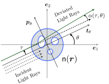
In this simplified model, the 2-D RIM is measured by , the sinus of the deflection angle of a light ray , where is the affine parameter determining the distance between and the origin, is the incident angle of with the axis, and is the (constant) perpendicular vector to the light ray direction .
The simplified ODT model depicted in Fig. 1-(top) is then obtained from the light ray equation (1) as
| (2) |
where is the (constant) reference refractive index of the surrounding medium, and the Dirac distribution turns the line integral into an integration over . In short, the above equation relates the deflection angle to the Radon transform of the transverse gradient of within the straight line trajectory approximation. Interestingly, this first order deflectometric model is also used in computer graphics for rendering of refractive gas flows [2].
As for traditional parallel absorption tomography [25, Section 3.2, p. 56], there exists a Deflectometric Fourier Slice Theorem (DFST) that relates the 1-D (radial) Fourier transform of the deflection angle along the affine parameter , i.e.,
| (3) |
to the 2-D Fourier transform of the RIM. Mathematically, the DFST establishes the following equivalence [22] (proved in Appendix A):
| (4) |
where stands for the 2-D Fourier transform of . Hereafter, the value is called affine frequency.
We may remark from (4) that there are different ways to cover the 2-D frequency plane with deflectometric measurements. This can be observed from the following symmetry relations for , , :
| (5a) | ||||
| (5b) | ||||
| (5c) | ||||
where the two first relations come from the change in (2) and (4), and the last equation is due to the Fourier conjugate symmetry of real spatial functions.
In particular, from the symmetry (5c), we can restrict to positive values by taking in the whole circle . Or alternatively, from (5b) and (5c), we can deduce and restrict to the half circle with . We insist on the fact that this symmetry is only preserved when the first order approximation is validated.
When comparing the relation (4) with the standard tomographic Fourier Slice theorem (FST) [25, Section 3.2, p. 56], the main difference is provided by the transverse gradient in the deflectometric relation (2), which results in multiplying by the RIM Fourier transform. In particular, from (2) or from (4) (since vanishes on the frequency origin) we see that the ODT sensing is blind to constant RIM. As we will see in Sec. 5, this implies that the RIM can only be estimated relatively to the known reference RIM .
Let us conclude by insisting on the impact of the equivalence (4). Similarly to the use of the Fourier Slice theorem in common (absorption) tomography, (4) is of great importance for defining a discrete ODT sensing model which can be computed efficiently in the Fourier domain given a discretized refractive index map .
2.2 Deflection Measurements
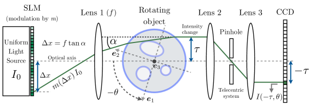
Experimentally, the deflection angles can be measured by phase-shifting Schlieren deflection tomography (schematically represented in Fig. 1-(bottom)). We briefly explain this system for the sake of completeness in order to set the experimental background surrounding the actual deflection measurement process. More details can be found in [24, 4, 18, 22].
This system proceeds by encoding light ray deflection in intensity variations. A transparent object is illuminated with an incoherent uniform light source modulated by a sinusoidal pattern using a Spatial Light Modulator (SLM). From classical optics, the light deviation angle is related to a phase shift , where is the focal length of Lens 1. This phase shift is associated with the intensity variation thanks to the modulation as . These intensity variations are processed by phase shifting methods for recovering the deflection measurements for each couple of parameters . Up to some linear coordinate rescaling, the affine parameter corresponds to the horizontal pixel coordinate in the 2-D CCD detector collecting light (assuming the object refractive index constant along the CCD vertical direction). This correspondence is implicitly allowed by the telecentric system formed by the combination of Lens 2 and 3. The pinhole guarantees that only parallel light rays outgoing from the object are collected. Rather than rotating the whole incident light beam around the object, it is this one which is rotated by an angle along an axis parallel to the CCD pixel vertical direction [4]. Finally, since the system is invariant under time inversion, i.e., under light progression inversion, measuring the deflection angle in Fig. 1-(bottom) is equivalent to measuring the same angle in Fig. 1-(top).
3 DISCRETE FORWARD MODEL
In order to reconstruct efficiently the RIM from ODT measurements, recorded data must be treated appropriately considering, jointly, the data discretization, the polar geometry of the ODT sensing and unavoidable measurement noises. We present here the discrete formulation of the ODT sensing and the construction of the forward model from the recorded data.
3.1 Discrete domains
Let us first assume that the object of interest is fully contained in a square field-of-view (or FoV) centered on the spatial origin. The physical dimensions of this FoV can be provided by the Deflectometric device itself. In other words, the RIM is constant and equal to the reference index outside of . This involves also that the deflection measurement vanishes, i.e., , if is bigger than the typical width of in a section of direction .
We can consider a spatial sampling of as follows. We define a 2-D Cartesian grid of pixels as
where the spatial spacing is adjusted to and to the resolution by imposing .
Second, as the deflectometric experiments provide evenly sampled variables and , is measured on a (signed) regular polar coordinate grid
of size , with the number of parallel light rays passing through the object (assumed even), the number of incident angles in ODT sensing, and the distance between two consecutive affine parameters and angles respectively444Notice that is not set to since is allowed to be negative..
The value can be known experimentally from the pixel size of the CCD detector in a Schlieren Deflectometer (Sec. 2.2). Moreover, the value and the resolution are also related to the FoV so that . Since there is no reason to ask more resolution to the sampling than the available in the affine variations of the ODT measurements, we will work with and .
Third, in this discretized setting, the affine frequency in (4) must also be sampled with values. As described in the next section, this comes from the replacement of the (radial) Fourier transform in (3) by its discrete counterpart. This leads to a (signed) frequency polar grid of same size
with . As it will become clearer in the following, only half of this polar grid will be necessary to bring independent observations of the RIM, i.e., we will often work on
with .
3.2 Discretized Functions
From the discrete domains defined above, the continuous RIM observed in the experimental FoV is discretized into a set of values from the coordinates . This description can always be arranged into a one dimensional -length vector , given a convenient mapping between the components indices of and the pixel coordinates in . This “vectorization” provides us a simplified representation of any linear operator acting on the sampled RIM as a matrix multiplying .
For the different functions discretized on or on , we use the same vectorization trick, namely, a function defined on and sampled on is associated to a vector with the right correspondence between the components of and the polar coordinates in (and similarly for function defined in the Fourier domain and sampled on ).
Therefore, the ODT observations are gathered in a vector with for a certain index mapping . In this discrete representation, the equivalent transformation of (3) reads
| (6) |
where is associated to a (vectorized) sampling of on , and performs a 1-D DFT on the radial -variations of , i.e.,
for a vectorized index . In other words, if is sufficiently small, e.g., if is band-limited with a cut-off frequency smaller than , then
using a Riemann sum approximation of (3) and knowing that vanishes on .
Despite the fact that belongs , this vector brings only independent real observations of . This is due to the central symmetry (5c) induced by the realness of and which allows us to consider only on .
This is clarified by the definition of the useful operator which perform the two following linear operations. First, it restricts any vector to the indices associated to the half grid . Second, it appends the imaginary values of the restricted vector to its real values in order to form a -length vector in . The adjoint operation , which is also the inverse of for vectors in respecting the Hermitian symmetry, is obtained easily by first reforming a -length complex vector from the separated real and imaginary parts, and by inserting the results in according to the indices of and by completing the information in with the central symmetry (5c).
Consequently, thanks to , we can form the real vector
| (7) |
with . We call the Frequency Deflectometric Measurements (FDM) vector. This will be our direct source of ODT observations instead of .
3.3 Forward Model
We can now explain how we use the DFST relation (4) for defining the forward model that links any discrete 2-D RIM representation to its FDM vector.
In a previous work [22], the data available in the frequency polar grid were first interpolated to a Cartesian frequency grid in order to reconstruct the 2-D RIM using a Fast Fourier Transform (FFT). However, the polar to Cartesian frequency interpolation introduced a hardly controlled colored distortion.
We use here another operator performing a non-equispaced Discrete Fourier Transform (NDFT) for directly relating functions sampled on the Cartesian spatial grid to those sampled on the polar frequency grid .
More precisely, given a function sampled on , the NDFT555This NDFT formulation is strictly equivalent to the one given in [26] where . computes
| (8) |
on the nodes of . Gathering all the values of and into vectors and respectively, this relation is conveniently summarized as
| (9) |
where the matrix stands for the linear NDFT operation. Its internal entry indexing follows the one of the components of and . We explain in Appendix B how the Non-equispaced Fast Fourier Transform (NFFT) algorithm allows us to compute efficiently in the multiplications and for any and , with a controlled distortion with respect to the true NDFT.
The action of on a discretized RIM is related to the continuous Fourier transform of as follows. Let be the point of the grid associated to the polar coordinates . Then, for a sufficiently small ,
| (10) |
To take into account the multiplication by in (4) and the existence of a factor in the equivalence (10), we introduce the diagonal operator defined as
where refers to the -coordinate of the point of , i.e., if as before is associated to then . The operator models the effect of the transverse gradient in the Fourier domain.
In parallel to the discussion ending Sec. 3.2, we also restrict the action of to the domain . Consequently, using the operator (Sec. 3.2), the final linear forward model linking the real FDM to the 2-D NDFT of the discrete RIM reads
| (11) |
The additional noise integrates the different distortions explained and estimated in Sec. 6, i.e., the numerical computations, the model discretization, the discrepancy to the first order approximation (2), and the actual noise corrupting the observation of .
Notice that in the absence of noise (), the model (11) could be easily turned into a classical tomographic model where the DC frequency is not observed. Indeed, forgetting the formal action of , if the frequency origin has been carefully removed from , then is invertible with , and we can solve the common tomographic problem
| (12) |
However, as we present in Sec. 8.1.1, this transformation is not suited to noisy ODT sensing. Even for a simple additive white Gaussian noise (or AWGN), the multiplication by breaks the homoscedasticity of , i.e., the variance of each varies with . This interferes with common reconstruction techniques used in classical tomography. Obviously, a noise whitening could be realized for stabilizing such methods but at least for AWGN, this strictly amounts to solve directly the model (11).
4 RELATED WORKS
This section describes some recently proposed methods for tomographic reconstruction in the domains of differential phase-contrast tomography and common absorption tomography.
In differential phase-contrast tomography, the refractive index distribution is recovered from phase-shifts measurements. These are composed by the derivative of the refractive index map, inducing the apparition of the affine frequency when using the FST, as it happens in the ODT sensing model (Sec. 2). In this application, Pfeiffer et al. [30] have used the FBP algorithm to reconstruct the refractive index map from a fully covered set of projections. Cong et al. [12, 11] have used different iterative schemes based on the minimization of the TV norm to reconstruct the refractive index distribution over a region of interest. These methods are accurate and provide similar results, but the iterative scheme based on the TV norm has proved to be better than FBP when the amount of acquisitions decreases.
In common Absorption Tomography (AT) we deal with the reconstruction of the absorption index distribution from intensity measurements. As these measurements are directly related to the absorption index, the AT sensing model does not include the affine frequency . In this domain, several works have exploited sparsity based methods. Most recent works in AT have focused on promoting a small TV norm [32, 34]. Sidky et al. [34] use a Lagrangian formulation for the tomographic reconstruction problem, promoting a small TV norm under a Kullback-Leiber data divergence and a positivity constraint. They aim at reconstructing a breast phantom from 60 projections with Poisson distributed noise. For this, they use the primal-dual optimization algorithm proposed by Chambolle et al. [9]. The method results in high quality reconstruction compared to FBP but with a convergence result that is highly dependent on the Lagrangian parameter choosen.
Ritschl et al. [32] use a constrained optimization formulation to reconstruct the absorption index from low amount of clinical data in the presence of metal implants and Gaussian noise. This problem is solved by means of an alternating method that allows then optimizing separately the raw data consistency function and the sparsity cost function, without the need of prior information on the observations. The fast convergence of the method is based on the estimation of the optimization steps. The gradient descent method is used to minimize the TV norm and the consistency term is minimized via an algebraic reconstruction technique. The method is proven to give better results than FBP.
These works have proved that some tomographic applications can be made compressive in the CS sense [6, 13]. In short, accurate tomographic image reconstruction are reachable from a number of samples that is smaller than the desired image resolution, if the image is sparse in some basis, i.e., the image expansion in that basis contains only a small number of nonzero coefficients. However, most of these works have considered Cartesian frequency grids while actual sensing often occurs in polar or non-equispaced grids. Besides, they attack different problems than ODT, where the sensing model and type of measurement change from one to the other. One important difference between AT and ODT sensing models, relies on the presence of the affine frequency as materialized by a diagonal operator ; whose impact is analyzed in detail in Sec. 6.2 and Sec. 8.1.1 for perfect and noisy sensing.
5 REFRACTIVE INDEX MAP RECONSTRUCTION
Three methods can be considered for recovering the discrete RIM : the common Filtered Back Projection (FBP); a penalized least square solution, which is related to a minimal energy solution (ME) [7]; and a regularized approach called TV- minimization. Since FBP and ME are widely used in tomographic problems, we will use them as a standard to compare with the quality of TV-.
Filtered Back Projection
The filtered back projection (FBP) can be briefly defined as an analytical method that consists of first filtering the tomographic projections with an appropriate function, i.e., a “ramp filter” for absorption tomography (AT) [25, Section 3.3, p. 60] or a simple Hilbert transform for deflection tomography [4, 30]. The result is then back projected in the spatial domain by angular integration. Despite its simplicity, this technique suffers of severe artefacts when the number of angular observations decreases. Moreover, FBP does not integrate the noise distortion in its processing.
Minimum Energy Reconstruction
Given a linear sensing model
| (13) |
of some image (vector) by a sensing operator with , a common procedure is to estimate by applying the (right) pseudo-inverse of to the observations, i.e., by computing (for non-singular ).
This solution is actually equivalent to compute a minimum energy solution (or penalized least square) by solving the convex problem
| (14) |
In words, the general inverse problem (13) is solved by a regularization promoting a small -norm (or energy). For large scale problems, solving this last convex formulation is preferred to the estimation of the pseudo-inverse that requires the costly inversion of a matrix.
Common reconstruction approaches (e.g., in Medical Imaging) follow this minimum energy principle [7]. They generally proceed by zeroing the Fourier coefficients of all unobserved frequencies, i.e., a process that minimizes the energy of the solution for frequency sampling defined on regular grids. The ME solution is also close to a discretization of the FBP procedure for a densely covered frequency space.
As shown later, the ME method presents some strong limitations when the model (13) is severely ill-conditioned or when noise corrupts the observation of . For instance, in the case where the tomographic problem subsamples a regular sampling of the Fourier domain, artifacts and bluring appear from the convolution of the pure image with the filter associated to the subsampling pattern (or dirty map [37]).
In ODT, the sensing operator and the sensing model read and , respectively, and we will denote by the corresponding ME solution.
TV- minimization
In order to overcome the limitations of both FBP and ME methods, we introduce a new reconstruction method which is both less sensitive to unwanted oscillations due to a low density frequency sampling and to additional observational noise in (11).
In particular, since the spatial dimensions in and in are expected to be equal, i.e., (Sec. 3.1) we are interested in lowering the density of in the Fourier plane by decreasing the number of angular observations . In other words, with respect to this reduction, we aim at developing a numerical reconstruction which makes Optical Deflectometric Tomography “compressive” in a similar way other compressive imaging devices which, inspired by the Compressed Sensing paradigm [6, 13], reconstruct high resolution images from few (indirect) observations of its content [15, 37, 34, 27]. This ability would lead of course to a significant reduction of the ODT observation time with potential impact, for instance, in fast industrial object quality control relying on this technology.
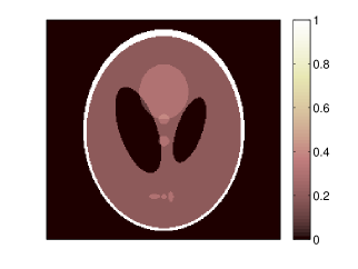
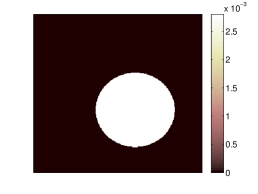
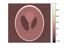
This objective of compressiveness can only be reached by regularizing the ODT inverse problem by an appropriate prior model on the configuration of the expected RIM . Interestingly, the actual RIM of most human made transparent materials (e.g., optical fiber bundles, lenses, optics, ..) is composed by slowly varying areas separated by sharp boundaries (material interfaces) (see Fig. 2-(left)). This can be interpreted with a Bounded Variation (BV) or “Cartoon Shape” model [33] as the typical Shepp-Logan phantom in Fig. 2-(right). Therefore, the inverse problem in (11) can be regularized by promoting a small Total-Variation norm, which in its discrete formulation is defined as [8]
where is the mixed norm defined on any as , and is the (finite difference) gradient operator. Reusing the 2-D coordinates of , this operator is defined along each direction as with and .
In order to obtain a reconstruction method which is also robust to additive observation noise, we must lighten the strict fidelity constraint implicitly used by the LS method in (14). Therefore, assuming the data corrupted by an additive white Gaussian noise (AWGN), we impose a data fidelity requirement using the -norm, i.e., if is known to have a bounded norm (or energy) , we force any reconstruction candidate to satisfy . The way can be estimated will be explained in Sec. 6.
Additionally to a fidelity criterion with the observed data, other requirements can be imposed on the reconstruction. First, we can often assume that the reference refractive index (i.e., the one of some optical fluid surrounding the object) is lower than the object RIM. Second, if the object is completely contained in the field-of-view of the ODT experiment, we can force any candidate RIM to match on the boundary of , i.e., imposing for all indices belonging to the border of . These indices are associated to pixels for which at least one of the two 2-D coordinates is equal to either or . The corresponding index set is denoted for simplicity.
Gathering all these aspects, we could propose the following reconstruction program
denoting by the vector of ones, i.e., the unit RIM in , and recalling that stands for the restriction of the components of to .
However, the reconstruction can be slightly simplified by observing that the kernel of the sensing operator in ODT contains the set of constant vectors in . This is a consequence of the vanishing affine frequency (which mainly defines the action of ) on the frequency origin, or more simply, this relies on the occurrence of the RIM gradient in the deflection model (2).
Therefore, a change of variable does not disturb the previous reconstruction which can be recast as
| (15) |
remembering that the true RIM estimation is actually .
Without the frontier constraint (), the unicity of the solution is not guaranteed. In that case, for one minimizer , all the vectors of also minimize the problem since the kernels of both and contain constant vectors. Considering the frontier constraint is thus essential for enforcing the unicity of the solution as expressed in the following lemma.
Lemma 5.1.
If there is at least one feasible point for the constraints of (15), then the solution of this problem is unique.
Proof.
Using the TV norm definition (and squaring it), the TV- optimization (15) is equivalent to solve
The kernel of is the set of constant vectors, while the one of (defining the frontier constraint) is the set of vectors equal to 0 on . Therefore, . Moreover, since the domain of is , and since we assume at least one feasible point, (15) has at least one solution.
Let and be two distinct minimizers. Then, and while . Therefore, and . By the strict convexity of the function , writing for , involves
showing that , which also satisfies the convex constraints, is a better minimizer, which is a contradiction. ∎
Therefore, we see that the uniqueness is actually reached by the stabilizing condition making the optimization running outside of .
6 NOISE IDENTIFICATION, ESTIMATION AND ANALYSIS
In this section we first discuss about the different sources of noise and how to estimate the noise energy present in the experimental data. Then, we analyze the noise impact in both AT and ODT measurements.
6.1 Noise sources
When a real sensing scenario is being studied, such as the ODT, different sources of noise are present and they have to be considered when determining the global noise energy bound in (15).
First, we have the observation noise. Under high light source intensity, the images collected by a Schlieren deflectometer (Fig. 1-(bottom)), and used for computing the ODT deflections , are mainly affected by electronic noise such as the CCD thermal noise. This induces a noise in the measured deflection angles that can reasonably be assumed Gaussian and homoscedastic, i.e., with an homogeneous variance through all the measurements. By computing the 1-D Fourier transform of the ODT measurements using in (7) the corresponding noise remains Gaussian [29] in the FDM , i.e., . Actually, from the orthonormality of the Fourier basis, (7) provides , where is the variance of the noise present in the ODT measurements (). This one can be estimated from the noisy observations using the Robust Median Estimator [14, 36].
Finally, this noise, defined as the difference between the noisy FDM and the noiseless FDM , has an energy that can be bounded using the Chernoff-Hoeffding bound [21]:
with high probability for .
Second, there is the modeling error that comes with every mathematical discrete representation of a physical continuous system. In the ODT system, this error is due to (i) the first order approximation used to formulate (2), (ii) the sampling of the continuous RIM and (iii) the discrete model itself. The modeling noise is related to the difference between the noiseless FDM and the sensing model , where performs the exact Polar Fourier Transform. As explained in Sec. 2.1, the modeling noise can be estimated by means of a ray tracing method based on the Snell law (not detailed here). This shows that for simple objects, an absolute error of is expected on light deflections smaller than . A Gaussian noise model provides a rough estimation of dB for the corresponding measurement SNR. This is equivalent to:
| (16) |
Third, we must consider the interpolation noise given by the mathematical error committed by estimating the polar Fourier Transform with the NFFT algorithm, i.e., the noise . To determine a bound on the energy of this error we first estimate the NFFT distortion (i.e., without the action of ), defined as the difference between the NFFT polar Fourier Transform and the true NDFT . Theoretically, for any vector , the -norm of this distortion is bounded as , where controls both the accuracy and the complexity of the NFFT [26] (see Appendix B). Assuming that each component of is iid with a uniform distribution , and using the Chernoff-Hoeffding bound [21, 23], we can estimate with high probability for . Finally, can be crudely computed as
with representing the maximum frequency amplitude in . In practice, because of the RIM shift explained in Sec. 5, we can bound and hence with the expected RIM dynamics , i.e., , and we adjust in order to have much lower than the other sources of noises.
Finally, we may also have an error introduced by the instrument calibration, when determining the exact and associated to the projections. We are going to neglect this error by assuming a pre-calibration process that provides an exact knowledge of these values (see Sec. 8.2).
In conclusion, gathering all the previous noise identifications and assuming the different noise are of zero mean and independent of each other, we can bound the difference between the actual ODT measurement and the sensing model as follows:
Therefore, we have .
6.2 Comparative study of the noise impact on AT and ODT
As we have seen in Sec. 3.3, the main difference between the AT and ODT problems is the appearance of the diagonal operator in the last one. Therefore, the AT sensing operator is described as and the ODT sensing operator as . We will now analyze the impact of an additive white Gaussian noise on the measurements regarding the presence of this operator.
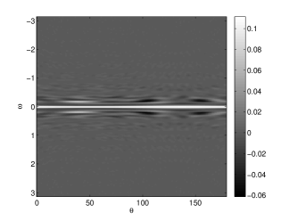
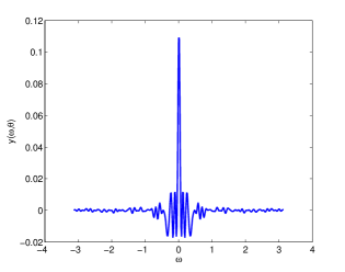
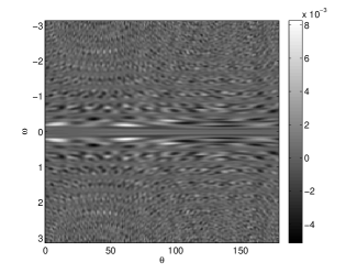
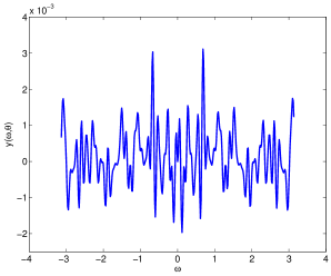
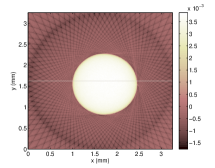
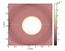
For this, we apply the sensing operators and to a section of the fibers bundle (see Fig. 5-(left)), in order to obtain the AT and ODT acquisitions, respectively. In Fig. 3 and Fig. 4 we show the real part of the Fourier measurements in AT and ODT.
For the class of images we are interested in, we can notice than in AT the magnitude presents a peak around and then decreases significantly when the distance to the center increases, tending to zero in the borders (see Fig. 3). Whereas in ODT, the presence of operator makes the image intensity to be quite spread through all the pixels (see Fig. 4). This has a direct impact on the reconstruction when the measurement is affected by additive Gaussian noise. As the noise spreads evenly through the image, the pixels that are not around will be more affected in the AT model because their intensity is significantly lower.
7 NUMERICAL METHODS
This section provides first an overview of the Chambolle-Pock primal-dual algorithm [9] used for solving (15) and hence recovering the RIM from the noisy FDM. The algorithm is then generalized into a product space optimization that allows the minimization of more than two convex functions. We show next how to use this generalization to solve our ODT problem under multiple constraints, before to briefly present an adaptive selection of the optimization parameters due to [19] offering faster convergence speeds.
7.1 Chambolle-Pock Primal-Dual Algorithm
The Chambolle-Pock (CP) algorithm (Algorithm 1 in [9]) is an efficient, robust and flexible algorithm that allows to solve minimization problems of the form:
| (17) |
for a linear operator and any variable . The functions and belong to the functional sets and , respectively.
In short, CP solves the primal problem described above simultaneously with its dual problem, until the difference between their objective functions – the primal-dual gap – is zero.
For any variable , the primal-dual optimization can be formulated as the following saddle-point problem:
| (18) |
where is the convex conjugate of function provided by the Legendre transform .
Using the Legendre transform we obtain the primal version described in (17) and also the dual version as follows:
| (19) |
where is the exact adjoint of the operator , such that .
The CP algorithm is defined by the following iterations:
| (20) |
The quantity denotes the proximal operator of a convex function for a certain finite dimensional vector space [10, 28]. This operator is defined as:
The proximal operator admits the use of non-smooth convex functions as the TV norm, making the algorithm suitable to solve the TV- problem described in Sec. 5.
Most numerical methods require operator being in a tight frame, which is not the case for our sensing operator . The CP algorithm reduces the convergence requirements, since we only need to tune the step sizes and such that the condition is true for any operator . Moreover, as presented in Sec. 7.4, these two parameters can be adaptively tuned during the iterations in order to reach faster convergence [19].
There is an easy way to estimate the convergence of the primal-dual algorithm (20). This relies on evaluating the primal and dual residuals defined by the subgradient of the saddle-point problem (18) with respect to the primal and dual variables, namely, and , respectively [19].
By definition, for an optimal point () of (18), zero must belong to these residuals and, therefore, by tracking the size of these residuals we can perform an analysis of the algorithm convergence. Explicit formulas can be obtained for the primal and dual residuals by observing the optimality conditions of (20) at each iteration. This provides
or, equivalently, and with the primal and dual residual vectors
| (21) |
Goldstein et al [19] show experimentally that a converging algorithm respects
| (22) |
for some norm (e.g., ). We will analyze the same convergence measure during our experiments in Sec. 8.
7.2 Product Space Optimization
In this paper, we are interested in minimization problems containing more than two convex functions. In particular, we aim at solving the general optimization
with and the number of convex functions. Such a problem does not allow the direct use of the CP algorithm as described before. However, it is easy to adapt it by considering a -times expanded optimization space . This space is composed of , with . In this context, we define bisector planes in order to work with the following equivalent primal problem:
| (23) |
The CP-shape (17) is thus recovered by working in this bigger space and by setting , with and , and .
In this expanded optimization space, the equivalent dual problem is written (see Appendix C.1):
For the functions described above, it is easy to see that for any and we have:
and, for any we have (more details in Appendix D.1):
7.3 ODT numerical reconstruction
Now we need to transform our TV- problem into an expanded form in order to use the CP algorithm. Having two constraints, the optimization space needs to be expanded by . Using (23), we can reformulate the primal problem from (15) as
| (24) |
where and . We show easily that (24) has the shape of (23) with for , for , , and .
For building the dual problem, we need the conjugate functions of , and , which are easily computed using the Legendre transform. As a matter of fact, is the indicator function onto the convex set with the mixed -norm defined as [9]. The conjugate function is computed as (see Appendix. C.2)
while the convex conjugate of is simply , where .
The dual optimization problem is thus defined as:
In order to apply (20), we must compute the proximal operators of , and . The one of is given by [9]
The proximal operator of is determined via the proximal operator of by means of the conjugation property defined in [10]:
The proximal operator of is given by the projection onto the convex set :
The proximal operator of the function represents a projection onto the positive orthant with zero borders:
Finally, making use of the above computations and taking , the CP algorithm applied to our TV- problem in ODT can be reduced to (see Appendix D.2)
| (25) |
In our experiments, the variables , and are initialized to zero vectors and the variable is initialized with the FBP solution as .
The algorithm presented in (25) stops when it achieves a stable behavior, i.e., when . The threshold is defined for ODT in the next section. In parallel, we analyze the convergence of the algorithm by means of the primal and dual residuals as described in (21). For the iterates in (25), the primal and dual residuals are defined as:
| (26) |
In order to guarantee the convergence of the algorithm, i.e., to ensure that converges to the solution of (15) when increases, we need to set and such that . The induced norm of the operator () was computed as explained in [34] using the standard power iteration algorithm to calculate the largest singular value of the associated matrix .
7.4 Adaptive optimization procedure
Until now, a non-adaptive optimization method, i.e., with constant step-sizes and , has been considered. However, such a procedure often presents slow convergence as presented in Section 8. Therefore, motivated by the recent work by Goldstein et al. [19], an adaptive version of the CP algorithm is used for the ODT reconstructions (See Algorithm 1). While this variant also depends on a couple of parameters that adjust the algorithm adaptivity, these are more naturally related to the characteristics of the inverse problem solved by this optimization.
In this adaptive approach, the stepsize update are tuned to the size of the primal and dual residuals at each iteration. If the primal residual is large with respect to the dual residual, then the primal stepsize is increased by a factor , and the dual stepsize is decreased by the same factor. If the dual residual is large with respect to the primal residual, then the primal stepsize is decreased and the dual stepsize is increased. The parameter is a constant that controls the adaptivity level of the method, and it is updated as , for some . In Algorithm 1, the parameter is used to compare the sizes of the primal and dual residuals and the scaling parameter , which depends on the image expected dynamics, is used to balance the residuals. The specific values selected for the parameters of Algorithm 1 are those recommended by [19].
8 EXPERIMENTS
In this section, the ODT reconstruction is first compared to the common tomographic (AT) reconstruction using the FBP and ME methods. Then, the proposed regularized reconstruction (TV-) is compared with the FBP and ME procedures on synthetic and experimental ODT data.
8.1 Synthetic Data
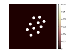
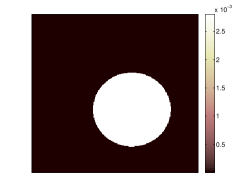
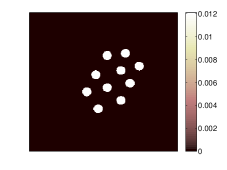
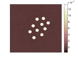
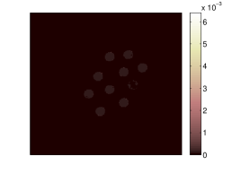
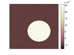
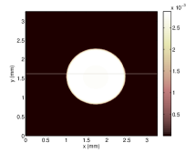
Three kinds of discrete synthetic 2-D RIM are selected to test the reconstruction. They are defined on a pixel grid (). In the first object, the RIM () simulates a 2-D section of a bundle of 10 fibers of radius 8 pixels each, immersed in an optical fluid (the background). The two media have a refractive index difference of (see Fig. 5-(left)). The second object consists in a homogeneous ball centered in the pixel with a radius of 60 pixels, immersed in a liquid with (see Fig. 5-(right)). These two objects were selected in correspondence to the available experimental data we use for reconstruction later in this section. The third object is the well-known Shepp-Logan phantom (see Fig. 2-(right)), which is a more complex image in a “Cartoon-shape” model.
The measurements were simulated according to (11) by means of the operator , and then, additive white Gaussian noise is added in order to simulate a realistic ODT scenario.
The operator is defined as , with representing the distorsion of regarding a true operator that would provide the actual NDFT. As discussed in Sec. 3.3, the NDFT computational time is inversely proportional to this parameter in . Therefore, we need to do a compromise between an accurate and an efficient computation of the NDFT. For this reason we use two different operators: (i) an accurate and high dimensional operator for the acquisition, with a small ; and (ii) a less accurate but lower dimensional operator for the reconstruction, with . The error caused for using a higher for the reconstruction is taken into account in (see Sec. 6).
For each object, the ODT measurements are obtained with according to a varying number of orientations , which allows to analyze the compressiveness of the reconstruction method. In this synthetic experiment, the orientations are taken in so that corresponds to two orientations per degree. Hereafter, we consider this last situation, i.e., as a “full observation” scenario since, given the considered RIM resolutions, the discrete frequency plane is almost fully covered in this case. More generally, we say that a given orientation number is associated to of the full coverage, being the number of orientations for having .
The reconstruction robustness with respect to the noise level has been considered for a Measurement SNR taken in . This last case with MSNR close to corresponds to the noiseless scenario, where no Gaussian noise is added, only the NFFT interpolation error () is taken into account. This actually provides a high MSNR value around .
The reconstruction quality of is measured using the Reconstruction SNR (RSNR) measured by
8.1.1 Robustness comparison for AT and ODT
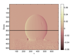
In order to assess numerically the impact of operator in ODT, we compare the RSNR between AT and ODT in similar noisy acquisition scenarios. The comparison is made using the FBP and ME procedures, commonly applied in tomographic reconstructions. In ODT the mean of the image cannot be estimated but this is not taken into account by FBP and ME procedures, thus the mean of the reconstructed image was removed for the computation of the RSNR in order to correctly compare the two reconstructions. We analyze the impact of the affine frequency , present in ODT, via the compressiveness and noise robustness. For this, we focus on the reconstruction of the bundle of fibers for different number of orientations . The results are depicted in Fig. 6 and Fig. 7.

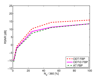

In Fig. 6 we can see that, when no Gaussian noise is added, we obtain similar RSNR for both AT and ODT. The same behavior is observed for both FBP and ME reconstructions, with FBP always providing a lower RSNR. The impact of the parameter is evident only in the convergence time of ME, causing the ODT reconstruction to be times slower than the AT one. However, when we add Gaussian noise in such a way that both data have a MSNR , the AT reconstruction presents a fast degradation while the ODT reconstruction remains almost unaffected by the noise (see Fig. 7). These results, observed for both FBP and ME, corroborate the discussion in Sec. 6.2.
Following the discussion from Sec. 3.3, we analyze now the reconstruction of the RIM using a simplified ODT sensing model that is close to a classical tomographic model (12). In Fig. 7 we show a third curve that corresponds to the RIM reconstruction from a noisy ODT sensing where the Fourier measurements are divided by the diagonal operator (ODT) as in (12). The results were obtained using the FBP and ME procedures and for a MSNR . As it was expected, when dividing the measurements by the operator , the reconstruction quality decreases significantly compared to the results obtained with the complete ODT sensing model (11). Moreover, the regularized formulation TV- cannot be used for this ODT reconstruction because the noise is then heteroscedastic.
8.1.2 TV- Reconstruction method
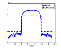
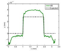
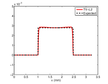
The TV- reconstruction is compared with the common FBP and ME methods. The reconstruction quality is investigated with respect to compressiveness and noise robustness. On the contrary of FBP and ME, the TV- method takes into account the zero mean of the image by the frontier constraint. Therefore, the mean of the reconstructed image is only removed from the ME and FBP results. Fig. 8 presents comparison graphs of FBP, ME and TV- showing the RSNR vs the number of orientations for the three noise scenarios. These results correspond to the reconstruction of the bundle of fibers for .
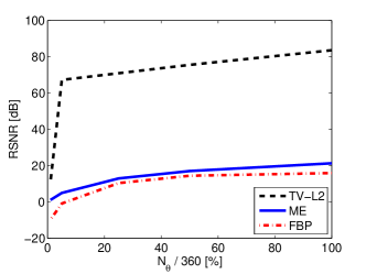
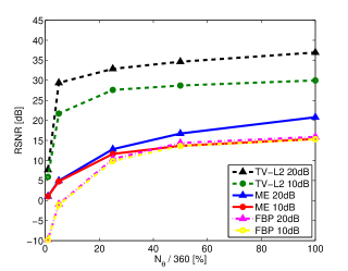
In Fig. 8-(left) we present the scenario without added noise, i.e., MSNR . We can see that for a full coverage, i.e., , as the TV- method takes into account the small noise coming from the NFFT interpolation error, it provides a very good reconstruction that outperforms by 62 dB the ME reconstruction quality and by 68 dB the FBP reconstruction quality.
Both FBP and ME methods degrade rapidly when the problem is ill-posed, i.e., when the projections space is not fully covered, whereas the TV- method maintains a high performance. By promoting a small TV-norm, the regularized method presents high compressiveness, as it can be observed in the graph where a high reconstruction quality is still achieved at only 5% of 360 incident angles, obtaining a gain of 62 dB over ME and of 68 dB over FBP. Although the performance of the algorithm decreases significantly for a coverage of 1%, it still provides a higher reconstruction quality than both ME and FBP.
The high compressiveness properties of the TV- method are preserved when we add Gaussian noise. We are able to obtain good quality images even for a compressive and highly noisy sensing. With TV-, at a MSNR , we get a RSNR of 22 dB for a 5% radial coverage compared to 5 dB for ME and -1 dB for FBP. However, we can notice how the reconstruction quality of TV- diminishes with respect to the noiseless scenario, whereas FBP and ME are less affected by the noise.
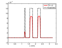
Fig. 9 presents the resulting images when reconstructing the bundle of fibers in a noiseless scenario and for , which represents, respectively, a coverage of and of the frequency plane. The algorithm is set to stop when is reached.
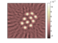

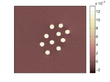
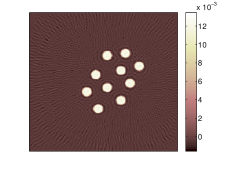
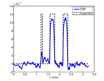
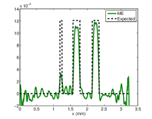
We notice how the TV- method preserves the image dynamics even for 5% of coverage, while FBP and ME provide images with implausible negative values. Moreover, at low measurement regime, some artifacts appear in both FBP and ME results. The image dynamics are less preserved in the FBP reconstruction, where the artifacts also affect the center of the fibers for a % of coverage.
About the numerical complexities, the FBP method takes less than 1 second for the reconstruction, while both ME and TV- methods require more time. For a coverage of 25% of the frequency plane, to reach the same stopping threshold value of , ME requires 6280 iterations (1h05’) while TV- requires 1900 iterations (28’). For a coverage of 5% of the frequency plane, the situation reverses and, to reach , ME requires 3450 iterations (51’) while TV- requires 6620 iterations (1h49’). However, the reconstruction quality is clearly higher when using our regularized method. In the case where the quality of the image reconstruction is sufficiently high, the threshold can be decreased to a less restrictive value. At the end of this section we perform a convergence analysis for different threshold values, which allows us to choose the suitable threshold for a required quality or convergence time.
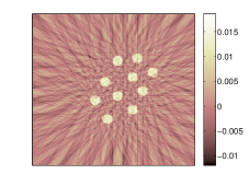
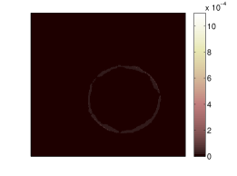
Although the FBP method requires less time than ME, we have noticed that the ME method outperforms FBP at low to medium reduction of the total number of angles. Henceforth, only the ME reconstruction method will be used for comparison with the TV- method. In Fig. 10 we present the reconstructed images for the bundle of fibers for a moderately noisy sensing (MSNR ). We also show the error images in order to provide a better appreciation of the difference between both methods.

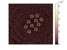
In this noisy scenario, the fiber contours are no longer well estimated using ME and, as we have coverage of only 25%, some oscillating (Gibbs) artifacts appear. On the contrary, the regularized method provides a good estimation on the borders, with no visible artifacts. We notice certain loss in the dynamics of the image, which causes a lower RSNR compared to the noiseless scenario.
Let us show now some results obtained for the other two synthetic images. Fig. 11 and Fig. 12 present the results obtained using ME and TV- on the sphere and the Shepp-Logan phantoms, respectively. This comparison was performed for and for , i.e., a coverage of of the frequency plane. As the image expected dynamics change for the Shepp-Logan phantom, the parameter for the residuals balancing was set to 250 instead of 1000.
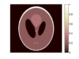

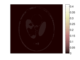
The regularized method provides a better image dynamics for these phantoms than when reconstructing the fibers for the same noise level. For these phantoms, it can also be observed that ME reconstructions present a poor estimation on the borders and oscillating artifacts. Moreover, the error image shows a higher discordance with respect to the actual image.
Table 1 presents a more complete comparison of the RSNR obtained using ME and TV- on the three synthetic images. The methods are analyzed for three scenarios, one noiseless with , and the other two with noise such that we have and . Results are presented for and , i.e., a coverage of of the frequency plane.
| TV- | ME | TV- | ME | TV- | ME | |
| Fibers | 70.9 | 13.1 | 39.02 | 12.83 | 35.69 | 11.63 |
| Sphere | 53.59 | 21.54 | 45.58 | 21.23 | 37.70 | 18.79 |
| Shepp-Logan | 54.37 | 13.21 | 36.85 | 13.04 | 25.24 | 11.79 |
When comparing the behavior of the algorithm for the different synthetic images, we can notice that TV- method outperforms the ME method for all cases.
8.1.3 Algorithm Convergence
Finally, we analyze the convergence of the algorithm by studying the evolution of the primal and dual residual norms and of the RSNR for different threshold values. We also analyze the convergence difference between the adaptive and the non-adaptive method. For this, only the reconstruction of the bundle of fibers for and MSNR = 20 dB is used, however, the other cases present a similar behavior.
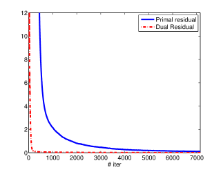
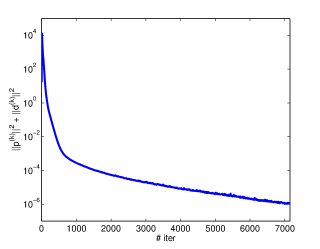
The evolution of the primal and dual residual norms (7.3) and the convergence condition in (22) along the iterations is depicted in Fig. 13. We notice that, when the number of iterations increases, the primal and dual residual norms tend to zero along with the energy ().
In order to compare the adaptive and non-adaptive methods, we analyze the evolution of and the RSNR along the iterations for two cases: (i) “Adapt” where the stepsizes are adaptively updated using Algorithm 1 and (ii) “Non-Adapt” where we use constant stepsizes equal to . Results are presented in Fig. 14.
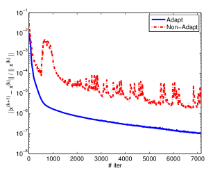
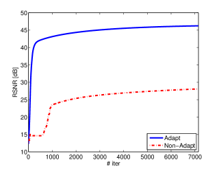
The evolution of helps us to analyze the stability of the algorithm. We can see the curves are not smooth specially for the non-adaptive method, which indicates a non stable behavior mainly due to a bad conditioning of the global operator in the product space optimization. This could be improved by a preconditioning procedure as described in [3, 31]. We also notice that for the same number of iterations, the adaptive method converges faster and provides a better result that the non-adaptive. Moreover, the adaptive method does not require to empirically set the parameters and as the algorithm will converge to the optimal parameters independently of the initialization.
Table 2 presents the values of the time and RSNR for different threshold values. These results show that a lower threshold provides higher reconstruction quality but significantly increases the number of CP iterations. In this specific reconstruction, setting the threshold to or running more than CP iterations guarantees a RSNR higher than dB.
| # iter | Time | RSNR [dB] | |
|---|---|---|---|
| 190 | 5’ | 38.79 | |
| 420 | 11’ | 41.86 | |
| 1540 | 42’ | 43.86 | |
| 7150 | 3h15’ | 46.24 |
8.2 Experimental Data
The reconstruction algorithm was tested with two particular transparent objects similar to the synthetic data studied in the previous section: a homogeneous sphere and a bundle of 10 fibers, both immersed in an optical fluid. The reconstruction is based on parallel and equally spaced light rays. The experimental setup is based on the Schlieren Deflectometric Tomography described in Sec. 2.
A pixels CCD camera was used for the acquisition, covering a field of view of . This corresponds to parallel light rays and 523 2-D slices, which leads to , and thus to .
Fig. 15 presents one measurement of the deflection angles on the CCD camera grid for the two analyzed optical phantoms. This observation corresponds to .
The experimental configuration leads to a calibration problem. As the object is rotating, the rotation center is modified within a small range and the origin of the affine parameter is altered. A post-acquisition calibration method was therefore implemented for correcting this effect. In short, for each angle, the method estimates the true centrum location by averaging the locations of the maximum and minimum deflection values along .
The two next paragraphs present the characteristics of the two objects of interest and the reconstruction results obtained for the three tested methods (FBP, ME and TV-) from the collected experimental observations. In all these experiments, and as discussed in Sec. 6.1, the TV- method was considered in the context of a 10 dB modeling noise. This choice seems somehow optimal for our experimental conditions. In several tests not reported here, higher or lower values of noise SNR lead either to severe artifacts in areas where no object is expected or to a significant loss in the expected RIM dynamics.
Homogeneous Sphere
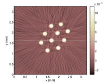
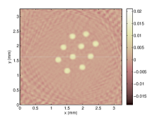
The first observed object consists of a homogeneous sphere with a diameter of mm. The difference of refractive index between the sphere and the optical fluid where it is immersed is . The deviation map was measured for angular positions over 360 degrees (i.e., 13% of measurements). The most important noise in the measurements is the modeling noise obtained by assuming MSNR = 10 dB (16), which provides ; while the estimated observation noise provides . The NFFT interpolation noise is considerably smaller, with . This noise estimation provides a MSNR = dB. Fig. 16 shows the reconstruction results obtained when using FBP, ME and TV- reconstruction methods, for the 300th 2-D slice of the observed 3-D object. The results are shown for a threshold , where ME converges in iterations and TV- in iterations.
We observe a similar behavior to the one found in the synthetic reconstruction. Compared to FBP and ME results, the sphere frontier is sharper with the TV- estimation and the RIM vanishes on the background. The image dynamics recovery is also more accurate using our regularized method, whereas with FBP and ME the reconstructions present several artifacts with implausible negative values. It is important to notice that the preservation of the image dynamics depends mainly on the noise estimation and on the proper definition of the constants included in the operator (see Sec. 3). When considering the appropriate constants, we are able to make an equivalence between the physical problem and its discrete mathematical formulation.
Bundle of fibers
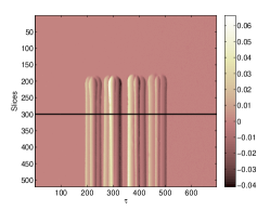
The second measured object is a bundle of 10 fibers of 200 m diameter each. The refractive index difference with respect to the solution where the fibers are immersed is . The experimental data was measured for 60 angular positions over 360 degrees (i.e., 17% of measurements). As in the case of the sphere, the noise that has more influence in the measurements is the modeling noise obtained by assuming MSNR = 10 dB (16), which provides ; while the observation noise provides . The NFFT interpolation noise is considerably smaller (). This noise estimation provides MSNR = dB.
Fig. 17 shows the reconstruction results obtained using FBP, ME and TV- reconstruction methods, for the 300th 2-D slice. For a threshold of , ME converges in 33920 iterations and TV- in 4560 iterations. Compared to FBP and ME reconstructions, TV- provides a much shaper estimation of the true RIM and the background is correctly estimated to 0. However, the image dynamics is not properly recovered. Such reconstruction error is present for the fibers because the refractive index difference between the material and the optical fluid is higher than for the sphere. In this case, the deflection angle is higher and it causes the modeling error to increase. The actual light ray trajectory could be estimated and inserted in an iterative process as done by Antoine et al. [1]. However, the forward model could not be represented in the frequency domain and we would loose its fast computation.

We can also notice that a section of the bundle of fibers represents a complex image to reconstruct, since the light enters and comes out of multiple fibers, and this amplifies the modeling error.
Furthermore, investigating the TV- program (15) and assuming that the unknown true RIM is a feasible point of the constraints, i.e., the noise power is correctly bounded, the TV-norm of the solution is necessarily smaller than the one of the true map. The norm reduction actually increases with the noise power since the optimization has then more freedom to reduce the TV-norm of the solution. A direct impact for cartoon shape maps is thus a reduction of RIM dynamics in the reconstruction compared to the expected one. Studying if this dynamics loss could be limited (e.g., by constraining the mean) is a matter of future study.
9 CONCLUSIONS
We have demonstrated how regularized reconstruction methods, such as TV-, can be used in the framework of Optical Deflectometric Tomography in order to tackle the lack of deflectometric observations and to make the ODT imaging process robust to noise. The proposed constrained optimization problem shows significant improvements in the reconstructions, compared to the well-known Filtered Back Projection and Minimum Energy methods. The results confirm that, when dealing with a compressive setting, the Total Variation regularization and the prior information constraints (positivity and FoV restriction) help in providing a unique and accurate estimation of the RIM, promoting sharp edges and preserving the image dynamics (when the modeling noise is limited). By working with the Chambolle-Pock algorithm we exploit the advantages of proximal operators and of primal-dual algorithms, and their flexibility to integrate multiple constraints. We have also shown that the use of the fast NFFT algorithm efficiently approximates (with a controlled error) the ODT sensing model involving the polar NDFT.
Noticeably, there still exist some artifacts in the experimental data reconstruction, coming from the modeling error. In order to handle this problem, we could no longer assume a linear light propagation. The actual curved light trajectories, depending themselves on the RIM through the eikonal equation, could be then traced. However, such a model improvement quickly leads to nonconvex optimization procedures and it breaks the fast computability of the forward sensing operator through the Fourier domain. Knowing how to insert this new scheme in our reconstruction method is a matter of future works.
Following the guidelines given in [19], the algorithm convergence is greatly improved by making CP adaptive. However, as the CP algorithm has been proved to work slowly when the problem is badly conditioned [3, 31], preconditioning our global operator can stabilize it and thus improve convergence results. We note also that most of the algorithms are implemented in Matlab, except for the NFFT algorithm which is compiled in C++. A faster implementation could be reached for instance by the adopting parallel (GPU) processing techniques, i.e., a framework particularly adapted to proximal optimization (e.g., see the UNLocBoX project666http://unlocbox.sourceforge.net). Such a numerical improvement will be mandatory for addressing 3-D RIM estimation. In this case, the whole (high dimensional) optimization driving the RIM reconstruction must to be considered in a (discretized) three dimensional space and fast forward model estimation will have to be developed.
We finally remark that the Optical Deflectometric framework treated in this paper can be also applied to other imaging techniques, such as the X-ray phase contrast tomography [30]. With the use of the energetic X-ray light, the first order paraxial approximation involving linear light trajectory is no longer needed and the proposed methods are expected to provide better results.
ACKNOWLEDGEMENTS
Part of this work is funded by the DETROIT project (WIST3/SPW, Belgium). LJ and CDV are funded by the F.R.S-FNRS.
Appendix A DEFLECTOMETRIC FOURIER SLICE THEOREM
Using the notations of Sec. 2.1, we must prove that
By definition of in (3), we have
However, for any function integrable on ,
Therefore, we compute easily for any ,
Setting and , we find finally
Appendix B NON-EQUISPACED FOURIER TRANSFORM
The non-equispaced Fourier Transform (NFFT) allows us to compute rapidly, i.e., in , the NDFT defined in (8) of a function defined on . This computation is performed with a controllable error which can be further reduced by increasing the computational time.
In a nutshell, the NFFT algorithm replaces the equivalent matrix multiplication of (9) by , where has fast matrix-vector multiplication computation. In this scheme, the discrepancy between and , as measured by , is controlled and kept small.
More precisely, the matrix starts by embedding in a bigger regular space of size , with . This is obtained from the multiplication of with a matrix that performs a weighting of by a vector (component wise) followed by a symmetric zero-padding on each side of the function domain . Once in , the common DFT matrix is applied. It can be computed with the FFT algorithm in order to obtained an oversampled Fourier transform of . Finally, a sparse matrix multiplies the output of in order to end in the dimensional space . Each row of corresponds to the translation in the 2-D Fourier domain of a compact and separable 2-D filter on one specific point of the non-regular grid . As a final result, the matrix is thus factorized in [26]
Without entering into unnecessary technicalities, the NFFT scheme is characterized by a precise connection between the function defining and the weighting performed by . In particular, each component of is actually set to the inverse of the Fourier transform of a filter , while is a periodization of (a truncation of) the same filter.
There exist several choices of windows / associated to different numerical properties (e.g., localized support in frequency and time, simple precomputations of the windows, …). We select here the translates of Gaussian bells [35], involving a Gaussian behavior for , which provides fast error decay for .
In particular, denoting by the oversampling factor and using the FFT for matrix-vector multiplications involving , the total complexity of the multiplications of or with vectors is
if we impose . For a fixed , this reduces to , which is far less than a direct computation of the DFT in computation even for small value of .
Appendix C CONVEX CONJUGATE FUNCTIONS
C.1 Convex conjugate of the function .
Given a vector , we can define the function , with the bisector plane . Therefore, for a vector , the dual function can be computed as follows:
C.2 Convex Conjugate of the indicator function .
Given the indicator function of the convex set , its dual function can be computed via the Legendre transform as follows:
The value of that maximizes the last expression is , and we get .
Appendix D DETAILS ON THE PRODUCT SPACE OPTIMIZATION
D.1 Proximal operator of the function
For every , the function is defined as:
where, for , denotes the bisector plane .
Then, for , the proximal operator of reduces to
As all the are equal, we necessarily have with defined by
with and where we used the fact that we can always subtract or add constants in the minimization without disturbing its solution. Denoting by the operator such that , this provides finally the compact notation
D.2 Formulation of Chambolle-Pock algorithm in OD
We take the CP algorithm as described in Eq. (20) and we translate it into our OD problem in the product space, to obtain the following:
We have the function and its proximal operator . As , we can relabel the variable as and . In the same way, , thus we can relabel the variable as and . We obtain the following algorithm:
References
- [1] P. Antoine, E. Foumouo, J.-L. Dewandel, D. Beghuin, A. González, and L. Jacques, Optical deflection tomography with reconstruction based on sparsity, Proc. of OPTIMESS2012, (Antwerp, Belgium), April 2012.
- [2] I. Ihrke, K. Berger, B. Atcheson, M. Magnor and W. Heidrich, “Tomographic reconstruction and efficient rendering of refractive gas flows.” Imaging Measurement Methods for Flow Analysis. Springer Berlin Heidelberg, 2009. 145-154.
- [3] S. Becker and J. Fadili, A quasi-newton proximal splitting method, preprint, arxiv:1206.1156, (2012).
- [4] D. Beghuin, J.L. Dewandel, L. Joannes, E. Foumouo, and P. Antoine, Optical deflection tomography with the phase-shifting schlieren, Optics Letters, 35 (2010), no. 22, 3745–3747.
- [5] M. Born, E. Wolf, and A.B. Bhatia, “Principles of optics: electromagnetic theory of propagation, interference and diffraction of light”, Cambridge Univ Press, 1999.
- [6] E.J. Candes and T. Tao, Near-optimal signal recovery from random projections: Universal encoding strategies?, IEEE Transactions on Information Theory, 52 (2006), no. 12, 5406–5425.
- [7] E.J. Candès, J. Romberg, T. Tao, Robust uncertainty principles: Exact signal reconstruction from highly incomplete frequency information, IEEE Transactions on Information Theory, 52 (2006), no. 2, 489-509, 2006.
- [8] A. Chambolle, An algorithm for total variation minimization and applications, Journal of Mathematical Imaging and Vision, 20 (2004), no. 1, 89–97.
- [9] A. Chambolle and T. Pock, A first-order primal-dual algorithm for convex problems with applications to imaging, Journal of Mathematical Imaging and Vision, 40 (2011), no. 1, 120–145.
- [10] P.L. Combettes and J.C. Pesquet, Proximal splitting methods in signal processing, Fixed-Point Algorithms for Inverse Problems in Science and Engineering, (2011), 185–212.
- [11] W. Cong, A. Momose, and G. Wang, Fourier transform-based iterative method for differential phase-contrast computed tomography, Optics Letters, 37 (2012), no. 11, 1784–1786.
- [12] W. Cong and G. Wang, Differential phase-contrast interior tomography, preprint, arxiv:1108.1414, (2011).
- [13] D.L. Donoho, Compressed sensing, IEEE Transactions on Information Theory, 52 (2006), no. 4, 1289–1306.
- [14] D.L. Donoho and J.M. Johnstone, Ideal spatial adaptation by wavelet shrinkage, Biometrika, 81 (1994), no. 3, 425–455.
- [15] M.F. Duarte, M.A. Davenport, D. Takhar, J.N. Laska, T. Sun, K.F. Kelly, and R.G. Baraniuk, Single-pixel imaging via compressive sampling, IEEE Signal Processing Magazine, 25 (2008), no. 2, 83–91.
- [16] F.X. Dupé, M.J. Fadili, and J.-L. Starck, Inverse problems with poisson noise: Primal and primal-dual splitting, IEEE International Conference on Image Processing (ICIP) (Brussels, Belgium), September 2011.
- [17] G. Faris and R. Byer, Beam-deflection optical tomography, Optics Letters, 12 (1987), no. 2, 72–74.
- [18] E. Foumouo, J.L. Dewandel, L. Joannes, D. Beghuin, L. Jacques, and P. Antoine, Optical tomography based on phase-shifting schlieren deflectometry, Proceedings of SPIE, 7726 (2010).
- [19] T. Goldstein, Esser E., and R. Baraniuk, Adaptive primal-dual hybrid gradient methods for saddle-point problems, preprint, arxiv:1305.0546v1 (2013).
- [20] A. González, L. Jacques, and P. Antoine, Tv- refractive index map reconstruction from polar domain deflectometry, 1st International Traveling Workshop for Interacting Sparse models and Technology (iTWIST’12) (Marseille, France), May 2012.
- [21] W. Hoeffding, Probability inequalities for sums of bounded random variables, Journal of the American Statistical Association, 58 (1963), no. 301, 13–30.
- [22] L. Jacques, A. González, E. Foumouo, and P. Antoine, Refractive index map reconstruction in optical deflectometry using total-variation regularization, Proceedings of SPIE, 8138 (2011).
- [23] L. Jacques, D. Hammond, and J. Fadili, Dequantizing compressed sensing: When oversampling and non-gaussian constraints combine, IEEE Transactions on Information Theory, 57 (2011), no. 1, 559–571.
- [24] L. Joannes, F. Dubois, and J.C. Legros, Phase-shifting schlieren: high-resolution quantitative schlieren that uses the phase-shifting technique principle, Applied Optics, 42 (2003), no. 25, 5046–5053.
- [25] A. C. Kak and Slaney M., “Principles of computerized tomographic imaging”, IEEE Press, 1988.
- [26] J. Keiner, S. Kunis, and D. Potts, Using NFFT 3—a software library for various nonequispaced fast fourier transforms, ACM Transactions on Mathematical Software (TOMS), 36 (2009), no. 4.
- [27] M. Lustig, D. Donoho, and J.M. Pauly, Sparse MRI: The application of compressed sensing for rapid MR imaging, Magnetic Resonance in Medicine, 58 (2007), no. 6, 1182–1195.
- [28] J.J. Moreau, Fonctions convexes duales et points proximaux dans un espace hilbertien. (French) [Dual convex functions and proximal points in a Hilbert space], CR Acad. Sci. Paris, 255 (1962), 2897–2899.
- [29] K. Morita, “Applied Fourier Transform”, IOS Press, 1995.
- [30] F. Pfeiffer, C. Kottler, O. Bunk, and C. David, Hard X-ray phase tomography with low-brilliance sources, Physical Review Letters, 98 (2007), no. 10.
- [31] T. Pock and A. Chambolle, Diagonal preconditioning for first order primal-dual algorithms in convex optimization, ICCV, (2011), 1762–1769.
- [32] L. Ritschl, F. Bergner, C. Fleischmann, and M. Kachelrieß, Improved total variation-based CT image reconstruction applied to clinical data, Physics in Medicine and Biology, 56 (2011), 1545–1561.
- [33] L.I. Rudin, S. Osher, and E. Fatemi, Nonlinear total variation based noise removal algorithms, Physica D: Nonlinear Phenomena, 60 (1992), no. 1-4, 259–268.
- [34] E.Y. Sidky, J.H. Jørgensen, and X. Pan, Convex optimization problem prototyping with the Chambolle-Pock algorithm for image reconstruction in computed tomography, preprint, arxiv:1111.5632, (2011).
- [35] G. Steidl, A note on fast fourier transforms for nonequispaced grids, Advances in Computational Mathematics, 9 (1998), no. 3, 337–352.
- [36] C. Taswell, The what, how, and why of wavelet shrinkage denoising, Computing in Science & Engineering, 2 (2000), no. 3, 12–19.
- [37] Y. Wiaux, L. Jacques, G. Puy, AMM Scaife, and P. Vandergheynst, Compressed sensing imaging techniques for radio interferometry, Monthly Notices of the Royal Astronomical Society, 395 (2009), no. 3, 1733–1742.
- [38] C. Zheng, J. Wu, and W. Sun, Applications of pseudo-polar FFT in synthetic aperture radar imaging, PIERS Online, 3 (2007), no. 1, 25–30.