Monte Carlo Integration with Subtraction

Abstract

This paper investigates a class of algorithms for numerical integration of a function in $d$ dimensions over a compact domain by Monte Carlo methods. We construct a histogram approximation to the function using a partition of the integration domain into a set of bins specified by some parameters. We then consider two adaptations; the first is to subtract the histogram approximation, whose integral we may easily evaluate explicitly, from the function and integrate the difference using Monte Carlo; the second is to modify the bin parameters in order to make the variance of the Monte Carlo estimate of the integral the same for all bins. This allows us to use Student’s $t$-test as a trigger for rebinning, which we claim is more stable than the $\chi^{2}$ test that is commonly used for this purpose. We provide a program that we have used to study the algorithm for the case where the histogram is represented as a product of one-dimensional histograms. We discuss the assumptions and approximations made, as well as giving a pedagogical discussion of the myriad ways in which the results of any such Monte Carlo integration program can be misleading.

1 Introduction

We are interested in evaluating the integral of a function $f:\mathbb{R}^{d}\to\mathbb{R}$ over a compact domain. It is a simple matter to map any compact domain into the unit hypercube, so we need to evaluate

$$I=\int_{[0,1]^{d}}dx\,f(x)=\int_{0}^{1}dx_{1}\cdots\int_{0}^{1}dx_{d}\,f(x_{1},\ldots,x_{d}).$$

$I$ is just the average value of $f$ over a uniform probability distribution which vanishes outside the unit hypercube, we denote this average value by $\langle f\rangle$.

Defining the sample average $\bar{f}$ over a set of $N$ uniformly distributed random points $\{x^{(i)}\in[0,1]^{d},i=1,\ldots,d\}$ to be

$$\bar{f}\equiv\frac{1}{N}\sum_{i=1}^{N}f(x^{(i)})$$ (1)

the weak law of large numbers [1] allows the identification $\langle f\rangle=\lim_{N\to\infty}\bar{f}$ assuming only that the integral exists. Strictly speaking the weak law of large numbers states that, with probability arbitrarily close to one, $\bar{f}$ will become arbitrarily close to $\langle f\rangle$ for sufficiently large $N$.

The central limit theorem makes the stronger statement that the probability distribution of $\bar{f}$ tends to a Gaussian with mean $\langle f\rangle$ and variance $V/N$,

$$\langle f\rangle=\bar{f}+{\cal O}\left(\sqrt{\frac{V}{N}}\right)$$ (2)

where the variance of the distribution of $f$ values is

$$V\equiv\left\langle\Bigl{(}f-\langle f\rangle\Bigr{)}^{2}\right\rangle=\int_{[0,1]^{d}}dx\,\Bigl{(}f(x)-\langle f\rangle\Bigr{)}^{2}=\langle f^{2}\rangle-\langle f\rangle^{2},$$

but it requires stronger assumptions that we shall discuss shortly. An unbiased estimate of the variance is given by

$$\hat{V}\equiv\frac{\overline{f^{2}}-\bar{f}^{2}}{N-1},\qquad\langle\hat{V}\rangle=V,$$

where of course

$$\overline{f^{2}}=\frac{1}{N}\sum_{i=1}^{N}f(x^{(i)})^{2}.$$

The estimate of the integral $\bar{f}$ is within one standard deviation $\sigma\equiv\sqrt{V/N}$ of the true value $I=\langle f\rangle$ about 68% of the time.

Note that the error is proportional to $1/\sqrt{N}$ independent of the dimension $d$ of the integral. From this fact stems the great utility of Monte Carlo for integration in many dimensions compared to numerical quadrature. Generally for numerical quadrature (trapezoid rule, Simpson’s rule etc.) the error is ${\cal O}(\Delta^{k})$ where $\Delta$ is the grid spacing and $k$ is a small number. With a fixed budget of function evaluations, $N$, on a regular grid each axis must be divided into $\root d \of{N}$ segments. So $\Delta\propto N^{-1/d}$ and thus the error is ${\cal O}(N^{-k/d})$; therefore in dimension $d>2k$ the Monte Carlo error is smaller. An intuitive explanation for this is that a random sample is more homogeneous than a regular grid [2].

1.1 Singular Integrands

If the integrand has a singularity within or on the boundary of the integration region extra care is required. Let us consider the proof of the central limit theorem. The probability distribution $P_{f}$ for the values $F=f(x)$ when $x$ is chosen from the distribution $P$ is

$$P_{f}(F)\equiv\int dx\,P(x)\,\delta\Bigl{(}F-f(x)\Bigr{)}$$ (3)

for which

$$\int dF\,P_{f}(F)=\int dx\,P(x)=1\qquad\mbox{and}\qquad\int dF\,P_{f}(F)\,F=\int dx\,P(x)\,f(x)=\langle f\rangle.$$

We define the generating function for connected moments as the logarithm of the Fourier transform of $P_{f}$

$$W_{f}(ik)\equiv\ln\int dF\,P_{f}(F)e^{ikF}=\ln\int dx\,P(x)e^{ikf(x)}=\ln\langle e^{ikf}\rangle.$$ (4)

Assuming that (4) can be expanded in an asymptotic series

$$W_{f}(k)=\sum_{m=1}^{\infty}\frac{k^{m}C_{m}}{m!}$$ (5)

where coefficients $C_{m}$ (cumulants)

$$C_{0} = 1$$

$$C_{1} = \langle f\rangle$$

$$C_{2} = V=\left\langle\Bigl{(}f-\langle f\rangle\Bigr{)}^{2}\right\rangle$$

$$C_{3} = \left\langle\Bigl{(}f-\langle f\rangle\Bigr{)}^{3}\right\rangle$$

$$C_{4} = \left\langle\Bigl{(}f-\langle f\rangle\Bigr{)}^{4}\right\rangle-3C_{2}$$

$$C_{5} = \left\langle\Bigl{(}f-\langle f\rangle\Bigr{)}^{5}\right\rangle-10C_{3}C_{2}$$

$$C_{6} = \left\langle\Bigl{(}f-\langle f\rangle\Bigr{)}^{6}\right\rangle-15C_{4}C_{2}-10C_{3}^{2}-15C_{2}^{2}$$

$$\vdots$$

are all finite. We consider the distribution function $P_{\bar{f}}$ for the sample average $\bar{f}$ defined in equation (1)

$$P_{\bar{f}}(F)=\int dx^{(1)}\cdots dx^{(N)}\,P(x^{(1)})\cdots P(x^{(N)})\,\delta\left(F-\frac{1}{N}\sum_{i=1}^{N}f(x^{(i)})\right)$$

and the corresponding generating function $W_{\bar{f}}$

$$W_{\bar{f}}(k)\equiv\ln\int dF\,P_{\bar{f}}(F)\,e^{ikF}.$$ (6)

Since the points $x^{(i)}$ were chosen independently (6) factorises to give

$$W_{\bar{f}}(k)=\ln\left[\int dx\,P(x)e^{ikf(x)/N}\right]^{N}=NW_{f}\left(\frac{k}{N}\right),$$

expanding which gives an (asymptotic) expansion in powers of $1/N$

$$W_{\bar{f}}(k)=\sum_{m=1}^{\infty}\frac{k^{m}C_{m}}{N^{m-1}m!}=kC_{1}+\frac{k^{2}C_{2}}{2N}+\frac{k^{3}C_{3}}{6N^{2}}+{\cal O}\left(\frac{1}{N^{3}}\right).$$

Ignoring terms of ${\cal O}(N^{-2})$ and taking the inverse Fourier transform gives

$$P_{\bar{f}}(F)=\frac{\exp\left(\frac{-(F-\langle f\rangle)^{2}}{2V/N}\right)}{\sqrt{2\pi V/N}},$$

namely a Gaussian with mean $\langle f\rangle$ and variance $V/N$.

However, if any of the moments $C_{n}$ are not finite then the expansion (5) is not justified. A simple class of integrals with divergent higher moments is $\int_{0}^{1}dx\,x^{\alpha}$ with $\alpha<0$. If $-1<\alpha<0$ this integral is well-defined but has an infinite number of divergent moments. Following equation (3)

$$P(y)=\int_{\epsilon}^{1}dx\,\frac{\delta(y-x^{\alpha})}{1-\epsilon}=\frac{y^{\frac{1}{\alpha}-1}}{\alpha(1-\epsilon)}$$

for $y\in[\epsilon^{\alpha},1]$, and zero elsewhere. The cumulants are combinations of the moments

$$\int dy\,P(y)y^{n}=\frac{1-\epsilon^{1+\alpha n}}{(1-\epsilon)(1+n\alpha)}$$

which diverge as $\epsilon\to 0$ if $1+\alpha n\leq 0$, or equivalently every cumulant $C_{n}$ with $n>-1/\alpha$ diverges. What this means in practice is that although estimating such integrals by Monte Carlo is allowed — the weak law of large numbers assures us that as long as $N$ is large enough the estimate will converge but it gives no indication of how large $N$ should be — it is misleading to estimate the error from the variance alone. This is because the distribution of the estimates of the integral is not Gaussian even if the variance exists. In practice one obtains non-Gaussian distributions with “fat tails”, for some examples see Figure 1.

We may also observe that a singularity in the integrand does not necessarily lead to infinite cumulants: for the function $f(x)=-\ln x$ a similar analysis to that given above shows that $P_{f}(F)=e^{-F}$ for $F\in[0,\infty)$ and hence $\langle f^{m}\rangle=m!$ so all its cumulants are finite, and therefore the Monte Carlo estimates of the integral do have a Gaussian distribution as the number of samples $N\to\infty$.

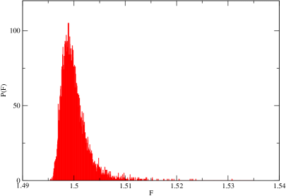
(a) $\int_{0}^{1}dx\,x^{-1/3}=3/2$

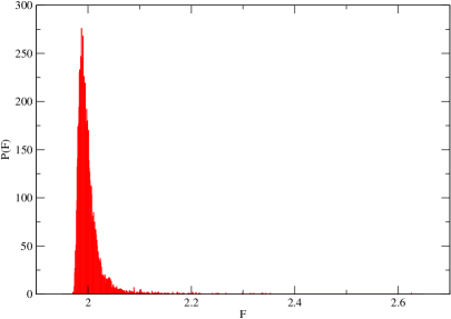
(b) $\int_{0}^{1}dx\,x^{-1/2}=2$

Figure 1: (a) $\int_{0}^{1}dx\,x^{-\alpha}$ with $\alpha={\mathchoice{\textstyle{1\over 3}}{\scriptstyle{1\over 3}}{\scriptscriptstyle{1\over 3}}{1/3}}$ and (b) $\alpha={\mathchoice{\textstyle{1\over 2}}{\scriptstyle{1\over 2}}{\scriptscriptstyle{1\over 2}}{1/2}}$ evaluated by Monte Carlo with $10,000$ function evaluations. The distribution of results about the mean is distinctly non-Gaussian. For (b), which has worse divergences, there is more weight in the tail of the distribution. For  (a) the variance exists but the distribution is not Gaussian due to the vanishing of the higher moments.

For all convergent integrals Monte Carlo provides an estimate of the mean. However, if any moment diverges the distribution of the means is not Gaussian, and in general even if the variance exists it gives an underestimate of the “width” of the probability distribution. This is often the case in practice, for example when evaluating Feynman parameter integrals which are integrable but not square integrable. If the Monte Carlo integrator is treated as a black box the quoted error from the standard deviation will often be an underestimate of the true error. With these provisos on the applicability of Monte Carlo integration we now turn to our main topic, a new method of adaptive Monte Carlo integration.

2 Variance Reduction

The Monte Carlo scheme of Section 1 (naïve Monte Carlo) can be improved by variance reduction schemes [3]: the basic idea is to use some information about the integral in order to reduce the variance sample average. We describe two methods: importance sampling and subtraction.

2.1 Importance Sampling

Let $\rho(x)$ be a probability distribution, normalised to one, that closely approximates our function over the interval. If we generate random points $x$ chosen from the distribution $\rho$ and construct the average $\langle f(x)/\rho(x)\rangle$ over these points then we have an estimate of the integral

$$I=\int dx\,f(x)=\int\rho(x)dx\,\frac{f(x)}{\rho(x)}$$ (7)

and the variance

$$V(\rho)\equiv\int\rho(x)dx\,\left(\frac{f(x)}{\rho(x)}-I\right)^{2}.$$ (8)

The value $I$ of (7) does not depend on $\rho$, but the corresponding variance of (8) does, so we may minimise the variance (8) by varying the function $\rho$ subject to the constraint that it is correctly normalised $N(\rho)\equiv\int dx\,\rho(x)=1$. Performing the required functional differentiation with the Lagrange multiplier $\lambda$

$$\frac{\delta[V(\rho)+\lambda N(\rho)]}{\delta\rho(x)}=0$$

we obtain the result

$$\rho_{\mbox{\tiny opt}}(x)=\frac{|f(x)|}{\int dx^{\prime}\,|f(x^{\prime})|}.$$

The corresponding value for the minimal variance is

$$V_{\mbox{\tiny opt}}\equiv V(\rho_{\mbox{\tiny opt}})=\left(\int dx\,|f(x)|\right)^{2}-\left(\int dx\,f(x)\right)^{2},$$ (9)

which vanishes if $f$ has the same sign everywhere in the domain of integration.

2.2 Subtraction

In this case we have

$$I=\int dx\,f(x)=\int dx\,[f(x)-g(x)]+\int dx\,g(x),$$ (10)

where the integral of $g$ is known exactly: the corresponding variance is

$$V(g)\equiv\int dx\,[f(x)-g(x)]^{2}.$$ (11)

As before the integral $I$ of (10) is independent of $g$ whereas the variance is not, so we may minimise the latter by varying $g$. This time there is no constraint to be imposed and we find

$$\frac{\delta V(g)}{\delta g(x)}=0\Rightarrow g_{\mbox{\tiny opt}}=f,$$

and the optimal variance $V_{\mbox{\tiny opt}}=V(g_{\mbox{\tiny opt}})=0$. We therefore choose $g(x)$ such that $g(x)$ is a good approximation to $f(x)$.

Both of these methods assume knowledge of the function that one may not have for complicated multidimensional integrals that arise in practice, thus it is necessary to find a way to construct $\rho$ or $g$ from a function treated as a black box.

3 Adaptive Algorithms

The usual way to construct $\rho(x)$ is the method of [4], VEGAS. The key feature of this algorithm is that it is adaptive, that is, it automatically constructs a probability density that approximates $|f(x)|$.

Our analysis of the variance reduction in §2.1 assumed that the function is representable as a product of functions in each variable, although the correctness of the global Monte Carlo estimate of the integral does not depend upon this. Such a factorisation depends on the co-ordinate system, see [5]: in the following we will always work in Cartesian co-ordinates and assume that the function approximately factorises.

Each axis is divided into a number of bins and we select a point with each coordinate lying equiprobably in any bin along the corresponding axis; the points are thus chosen to lie in equiprobably in any of the boxes that are defined by the intersection of the bins. The probability distribution $\rho$ in (7) is $\rho(x)=1/|b_{x}|$ where $|b_{x}|$ is the volume of the box $b_{x}$ containing $x$. To converge to the optimal grid the bins are resized so that each bin makes an equal contribution to the integral of $|f(x)|$.

The analysis in [4] assumes that the probability distribution $\rho(x)=\prod_{i=1}^{d}\rho_{i}(x_{i})$ factorises but does not explicitly assume that the integrand $f$ does. In this case the variance is

$$V(\rho)=\int\left(\prod_{i=1}^{d}\frac{dx_{i}}{\rho_{i}(x_{i})}\right)f(x)-I^{2},$$

and minimisation with respect to any particular $\rho_{i}$ subject to the normalisation constraint $N(\rho_{i})=\int dx_{i}\,\rho_{i}(x_{i})=1$ gives

$$\rho_{i,{\mbox{\tiny opt}}}(x_{i})\propto\sqrt{\int\left(\prod_{j=1\atop j\neq i}^{d}\frac{dx_{j}}{\rho_{j}(x_{j})}\right)f(x)^{2}}.$$

This gives the optimal solution for $\rho_{i}$ when all the other $\rho_{j}$ are fixed, but does not immediately give the optimal solution for all the factors of $\rho$ simultaneously. If we make the further assumption that $f(x)=\prod_{i=1}^{d}f_{i}(x_{i})$ then the solution reduces to that which we found in §2.1, namely $\rho_{i,{\mbox{\tiny opt}}}(x_{i})\propto|f_{i}(x_{i})|$ and hence $\rho_{\mbox{\tiny opt}}(x)\propto|f(x)|$.

We may identify some issues with this approach. Consider the optimal distribution $\rho_{\mbox{\tiny opt}}$ that VEGAS is trying to find. $V_{\mbox{\tiny opt}}$ of equation (9) is not necessarily zero unless $f(x)$ has the same sign everywhere. A simple example where $V_{\mbox{\tiny opt}}\neq 0$ is in one dimension with $f(x)=\sin 2\pi x$, which gives $V_{\mbox{\tiny opt}}=16$. In simple cases it is possible to divide up the integration region into parts in which the sign of the integrand does not change, however this assumes detailed knowledge of the function and may not be feasible in a high number of dimensions. Compare this to the subtraction method, for which $V_{\mbox{\tiny opt}}=0$ in this case.

Secondly, there seems to be no automatic method for deciding when VEGAS has converged to a (near) optimal grid. Usually it is advised to use as few function evaluations as possible until the grid approximately converges and then sample on the optimal grid. To test this one computes the $\chi^{2}$ statistic. If on each iteration of VEGAS an independent estimate of the integral $I_{i}$ is produced using $N^{\prime}$ function evaluations; after $n$ iterations the variables $(I_{1}-I),\ldots,(I_{n}-I)$ will have a normal distribution with mean zero and variance $\sigma^{2}$, assuming that $N^{\prime}$ is sufficiently large for central limit theorem to apply. Therefore the sum of their squares

$$\chi^{2}=\sum_{i=1}^{n}\left(\frac{I_{i}-I}{\sigma}\right)^{2};$$ (12)

has a $\chi^{2}$ distribution with $n$ degrees of freedom

$$P^{\chi^{2}}_{n}(\chi^{2})=\frac{(\chi^{2})^{\frac{n}{2}-1}e^{-\chi^{2}/2}}{2^{n/2}\Gamma\left(\frac{\nu}{2}\right)}$$

for $\chi^{2}\geq 0$. Sadly, we cannot compute this $\chi^{2}$ since it requires the exact values of $I$ and $\sigma$. If we use the estimate $\bar{I}\approx I$ then it is easy to show that the resulting quantity

$$\chi^{\prime 2}=\sum_{i=1}^{n}\left(\frac{I_{i}-\bar{I}}{\sigma}\right)^{2}$$

still has a $\chi^{2}$ distribution but now with $n-1$ degrees of freedom. However, since $\sigma^{2}$ occurs in the denominator of $\chi^{2}$ attempts to replace it with some stochastic estimate will tend to give anomalous large values for $\chi^{2}$ or, to make a more precise statement, the distribution will not be a $\chi^{2}$ distribution but something with fatter tails.

Finally, we observe that the VEGAS rebinning algorithm will tend to produce small bins where the function value is large. If the integrand has a relatively flat but high plateau with steep edges this approach will tend to calculate the integral well in the flat region, where it is easy, and miss the regions of large variance which require more function evaluations to estimate accurately. We will see an explicit example in section 5.

4 Our Algorithm

Our algorithm uses two adaptations, subtraction and rebinning, and uses Student’s $t$-test as a robust trigger to decide when to apply them.

As in all such adaptive algorithms, we trigger an adaptation whenever there is statistically significant evidence that the current histogram parameters are not optimal, and the naïve goal is that the histogram parameters will converge to their optimal values thereby minimising the variance of our Monte Carlo estimate of the integral. We say “naïve” because this clearly cannot happen: we are constructing an ergodic Markov process and such a process must converge to a fixed point distribution of histogram parameters which is non-zero everywhere — it cannot converge to a single point in the parameter space. Of course, we may hope that the Markov process will converge to a distribution of histogram parameters strongly peaked about the optimal ones, but how well this may be achieved depends in a complicated way upon lots of the algorithmic details and approximations: for example, how many samples we have to take in each bin before using the central limit theorem to assert that their mean is normally-distributed, or how much we choose to damp the rebinning adaptations to try to avoid instabilities.

We should put such worries in context, it is easy to see that for any adaptive Monte Carlo integration scheme there are functions for which they will give an answer with an unreliable estimate of its error. A simple example is an approximation to a $\delta$ function within a region where the function is zero: not only will Monte Carlo algorithms not “see” the $\delta$ function, but adaptive importance sampling will make it less likely for them to do so.

4.1 Subtraction Adaptation

We construct an approximation function $\hat{f}$ adaptively from the Monte Carlo process. Like [4] we assume that the integrand may be reasonably approximated by a product of one-dimensional histograms with $n$ bins along each axis. This means we only have to accumulate ${\cal O}(nd)$ rather than ${\cal O}(n^{d})$ values, and more significantly we can afford to evaluate a reasonably large number of samples per bin whereas it would be impossible to evalute even one sample per box in practice for $n=10$ in $d=10$ dimensions for example. However, we stress that the this is not a requirement of our method: the idea of using adaptive subtractions as well as adaptive importance sampling is independent of the choice of histogram representation. Subtraction could be used together with recursive stratified sampling [6] for example, and the function approximation stored not as a product of histograms as we will describe below but as independent values in each box as required.

We should also stress that the Monte Carlo algorithm will give the correct value for the integral even if the integrand is not well approximated by a product of histograms, or even as a product at all. All that happens in such cases is that we have no good reasons to expect our adaptations to significantly reduce the statistical error in the result.

We describe a method closely following VEGAS, assuming that our function is representable as a product of one-dimensional functions. Each axis is divided into a number of bins, with a bin along an axis defined to be the Cartesian product of an interval along that axis and the unit interval along every other axis. The intersection of $d$ bins, one along each axis, will be called a box.

We generate quasi-random points for the Monte Carlo sampling by choosing a random permutation of the bins and a random point in each bin. This ensures that each bin has an equal number of samples while still sampling the entire space homogeneously. This implements the importance sampling distribution $\rho$, as the probability of selecting a sample point $x$ within any box $b$ is $1/n^{d}$, and therefore the probability density $\rho(x)=1/V_{b}$ where $V_{b}$ is the volume of the box $b$. Initially we choose all the histogram bins to have equal width, and therefore all the boxes to have the same volume and therefore $\rho(x)$ equal everywhere, for want of any better information. Likewise, we initially set the subtraction function $\hat{f}(x)=0$ everywhere.

We generate a set $\{x^{(i)},\ldots,x^{(N)}\}$ of quasi-random points chosen from the distribution $\rho$, and for each bin $\beta_{\mu}\in\{1,\ldots,n\}$ along each axis $\mu\in\{1,\ldots,d\}$ we accumulate the quantities

$$\Sigma_{k}(\beta_{\mu})=\sum_{x^{(i)}\in\beta_{\mu}}\left(\frac{f(x^{(i)})}{\rho(x^{(i)})}\right)^{k}$$

for $k\in\{0,1,2\}$. $\Sigma_{0}(\beta_{\mu})$ is just the number of samples in the bin $\beta_{\mu}$, so with our quasi-random number strategy for generating sample points it is just equal to the integer $N/n$ for all bins, so we do not really need to accumulate it, although we might if we used a different random point generator. We define

$$\hat{f}_{\beta_{\mu}}\equiv\frac{\Sigma_{1}(\beta_{\mu})}{\Sigma_{0}(\beta_{\mu})}\approx\int_{x\in\beta_{\mu}}\rho(x)dx\,\frac{f(x)}{\rho(x)}=\int_{x\in\beta_{\mu}}dx\,f(x)$$

where $x^{(i)}\in\beta_{\mu}$ means that $x^{(i)}$ falls within $\beta_{\mu}$, that is the $\mu$ coordinate $x^{(i)}_{\mu}$ of the point $x^{(i)}$ lies in the interval $\beta_{\mu}$ along the $\mu$ axis.

If $f$ is a product of one-dimensional functions, $f(x)=f_{1}(x_{1})\cdots f_{d}(x_{d})$ then

$$\int_{x\in\beta_{\mu}}dx\,f(x)=\int_{\beta_{\mu}}dx_{\mu}\,f_{\mu}(x_{\mu})\prod_{\nu\neq\mu}\int_{0}^{1}dx_{\nu}\,f_{\nu}(x_{\nu});$$

moreover, if the average value of $f_{\mu}$ in the bin $\beta_{\mu}$ is

$$\langle f_{\mu}\rangle_{\beta_{\mu}}=\frac{1}{|\beta_{\mu}|}\int_{\beta_{\mu}}dx_{\mu}\,f_{\mu}(x_{\mu})$$

with $|\beta_{\mu}|=\int_{\beta_{\mu}}dx_{\mu}$ being the bin width, then

$$\hat{f}_{\beta_{\mu}}\approx\int_{x\in\beta_{\mu}}dx\,f(x)=\frac{\langle f_{\mu}\rangle_{\beta_{\mu}}|\beta_{\mu}|I}{\displaystyle\int_{0}^{1}dx_{\mu}\,f_{\mu}(x_{\mu})}$$

where

$$I=\int dx\,f(x)=\prod_{\nu=1}^{d}\int_{0}^{1}dx_{\nu}\,f_{\nu}(x_{\nu})$$

is the integral we wish to evaluate. We thus may construct an estimate of the value of the function $f(x)$ as

$$\hat{f}(x)=\prod_{\nu=1}^{d}\frac{\hat{f}_{\beta_{\nu}}}{|\beta_{\nu}|\hat{I}^{d-1}}=\frac{1}{V_{b}\hat{I}^{d-1}}\prod_{\nu=1}^{d}\hat{f}_{\beta_{\nu}}\approx\prod_{\nu=1}^{d}\langle f_{\nu}(x_{\nu})\rangle_{\beta_{\nu}}$$ (13)

where $x\in\beta_{\nu}$ for $\nu\in\{1,\ldots,d\}$, $V_{b}=|\beta_{1}|\cdots|\beta_{d}|$ is the volume of the box $b$ containing $x$, and

$$\hat{I}=\frac{1}{N}\sum_{i=1}^{N}\frac{f(x^{(i)})}{\rho(x^{(i)})}\approx I$$

is the current “global” estimator for the integral.

We use this function for our subtraction adaptation, that is we take $g=\hat{f}$ in (10), and evaluate

$$I^{\prime}\equiv\int dx\,[f(x)-\hat{f}(x)]=\int\rho(x)dx\,\frac{f(x)-\hat{f}(x)}{\rho(x)}$$ (14)

by Monte Carlo. The integral of $\hat{f}$ is known exactly

$$I^{\prime\prime}\equiv\int dx\,\hat{f}(x)=\frac{1}{\hat{I}^{d-1}}\prod_{\nu=1}^{d}\sum_{\beta_{\nu}=1}^{n}\hat{f}_{\beta_{\nu}},$$

whence we can use (10) and set $I=I^{\prime}+I^{\prime\prime}$.

4.2 Rebinning Adaptation

After making a subtraction as described in section 4.1 the integrand is everywhere approximately zero to the best of our current knowledge, so the usual importance sampling analysis of section 2.1 does not give us any useful way of choosing the function $\rho$. We may therefore choose $\rho$ so as to make the variance constant over all boxes, which in our case corresponds to making it constant for all bins along each axis. We introduce an estimator for the variance with the bin $\beta_{\mu}$

$$\hat{V}_{\beta_{\mu}}\equiv\frac{\Sigma_{0}(\beta_{\mu})}{\Sigma_{0}(\beta_{\mu})-1}\left(\frac{\Sigma_{2}(\beta_{\mu})}{\Sigma_{0}(\beta_{\mu})}-\hat{f}_{\beta_{\mu}}^{2}\right)\approx\int_{x\in\beta_{\mu}}\rho(x)dx\,\left(\frac{f(x)}{\rho(x)}-I\right)^{2},$$

and our rebinning step adjusts the bin parameters to make the integral of this histogram constant within each new bin. An interpolation is performed along each axis to get the value of the approximation function in the new bins. The interpolation uses cubic splines to fit the current function approximation in the current set of bins: cubic splines perform better for some of our test integrals than lower-order interpolation, although there is no intrinsic reason to prefer them. When the new set of bins have been found the value of the interpolation in the centre of that bin is used for $\hat{f}_{\beta_{\mu}}$. As with importance sampling it is possible that the algorithm will rebin too much and narrow the bins very strongly about regions of high variance, thus we damp the rebinning algorithm by adding a small constant variance to each bin so that no bin can have width zero. The second part of  (14) tells us how to make a subtraction even after changing the importance sampling $\rho$: we just keep the old bins to evaluate $\hat{f}$ (perhaps packaging them in a closure) while generating points according to the new bins specified by $\rho$. The value of $\hat{f}$ for the next iteration is accumulated in the new bins. Interpolation was easier to use in our current implementation and allows us to combine estimates from different iterations and avoid starting again after each rebinning.

4.3 Student Trigger

If our two adaptations have achieved their goal then the estimates $z_{\beta_{\mu}}$ of $[f(x)-g(x)]/\rho(x)$ within bin $\beta_{\mu}$ should have mean zero and equal variance, and if we average enough samples within each bin to be able to apply the central limit theorem then they should follow a Gaussian distribution. Even though we do not know the exact value of the variance, we can test this hypothesis without any further approximations by computing the quantity

$$t\equiv\frac{\mu_{z}}{\sqrt{V}_{z}}$$ (15)

where

$$\mu_{z}\equiv\frac{1}{nd}\sum_{\mu=1}^{d}\sum_{\beta_{\mu}=1}^{n}z_{\beta_{\mu}}$$

is the average of $z$ over all bins and

$$V_{z}\equiv\frac{1}{nd(nd-1)}\sum_{\mu=1}^{d}\sum_{\beta_{\mu}=1}^{n}(z_{\beta_{\mu}}-\mu)^{2}$$

an unbiased estimate of the variance of $\mu_{z}$. $t$ has a Student $t$-distribution with $nd-1$ degrees of freedom, where Student’s distribution with $\nu$ degrees of freedom is

$$P^{t}_{\nu}(t)=\frac{\left(1+\frac{t^{2}}{\nu}\right)^{-\frac{\nu+1}{2}}}{\sqrt{\nu}B\left(\frac{\nu}{2},\frac{1}{2}\right)}.$$

Let $k=A^{-1}(p,nd-1)$ where $A^{-1}$ is the inverse cumulative Student distribution, so we expect that $-k\leq t\leq k$ with probability $p$. Therefore, if $|t|>k$ we may exclude the hypothesis that we have Gaussian distributed bin values with mean zero and the same variance with probability $p$ and carry out a new adaptation. This should give a more stable condition for convergence towards the optimal approximation function. Each axis could have a separate trigger, but there does not seem to be any obvious advantage, just as there seems to be no reason to have a different number of bins $n$ along each axis.

The rebinning algorithm is a Markov process that is hopefully converging to the “optimal” bin distribution. However, as we stated before, an ergodic Markov process cannot converge to a delta function, so our automated rebinning procedure cannot find the optimal integration parameters (the bin widths and subtraction values). In practice this manifests itself as an instability in the rebinning algorithm. This is not a problem specific to our method but is shared by all automatic rebinning schemes; we hope and expect that our use of Student’s test as a trigger will be more stable that those that use a $\chi^{2}$ trigger, but to make this into a more quantitative statement would require at least a significant restriction on the class of integrands under consideration.

5 Numerical examples

\psfrag{t(x)}{\huge$t(x)$}\psfrag{x}{\huge$x$}\includegraphics[angle={-90},width=211.3883pt]{tanhprod_sub.eps}

(a) After adaptive subtraction

\psfrag{t(x)}{\huge$t(x)$}\psfrag{x}{\huge$x$}\includegraphics[angle={-90},width=211.3883pt]{tanhprod_imp.eps}

(b) After adaptive importance sampling

Figure 2: Rebinning with our algorithm (a) or importance sampling (b) for the integral (16) along with the function $t(x)-\hat{t}(x)$ where $\hat{t}$ is the approximation function adaptively constructed by our algorithm. The bin distribution for our algorithm concentrates the bins at the edges where the variance is largest.

\psfrag{log(s/f)}{\huge$\log(\frac{s}{\bar{t}})$}\psfrag{n}{\huge$n$}\includegraphics[angle={-90},width=375.80542pt]{tanh_dim.eps}

Figure 3: Log of the standard error over the integral evaluation calculated as described in the text for equation (17) versus dimension. In one dimension the subtraction method is many orders of magnitude better, in more than one dimension the subtraction method is still better than importance sampling. For this integrand, having fewer calls per bin is better for both subtraction and importance sampling.

To demonstrate the procedure of adaptive subtraction and how it compares to adaptive importance sampling, we use the C language implementation of VEGAS importance sampling in the GNU Scientific Library (GSL) for comparison [7]. We first choose an example that illustrates the strengths of our method,

$$I=\int_{0}^{1}dx\,t(x)\qquad\mbox{where}\qquad t\equiv N\tanh(15x)\tanh\Bigl{(}15(1-x)\Bigr{)}$$ (16)

with $N$ chosen to make the integral $I=1$. The integrand is approximately constant throughout most of the integration region except at the very edges where it rises rapidly. Figure 2(a) shows the integrand after subtraction with the new bins, chosen such that the variance in each is equal. The integration grid is finest in regions where the function is changing rapidly, this is as it should be, integrating regions where the integrand is approximately constant requires far fewer function evaluations. Compare to part (b) of the figure which shows the bin distribution produced by importance sampling. The bin distribution has moved to where the function itself is largest. We integrate,

$$\int_{[0,1]^{d}}dx_{1}\cdots dx_{d}\,t(x_{1})...t(x_{d})$$ (17)

for various values of $d$ and plot the relative error in Figure 3. This figure shows the log of the standard error over the integral approximation using importance sampling and our subtraction method. We use $8\times 10^{4}$ evaluations, with the number of bins chosen in both cases so that there are $10$ or $100$ calls per bin. This gives four opportunities to recalculate the bin distribution (rebin) where we apply Student’s test to decide. In almost every case, with $90\%$ probability only one rebinning is necessary. We also check the $\chi^{2}$ for the importance sampling case the same number of times and rebin if the $\chi^{2}$ per degree of freedom of the integral estimates differs from one by more than $0.5$. This tends to rebin on every step. We could combine all the estimates, weighted by their standard deviation however this sometimes underestimates the error. Instead the number we quote comes from $2\times 10^{4}$ calls on the bin distribution calculated by the process above. Figure 3 shows for this example our algorithm gives more accurate results.

\psfrag{tstat}{\huge$t$}\psfrag{cstat}{\huge$|\chi^{2}-1|$}\psfrag{chisq}{\large$|\chi^{2}-1|$}\psfrag{it}{\huge$Iteration$}\includegraphics[angle={-90},width=211.3883pt]{studentt_it.eps}

(a) Subtraction Method $t$-statistic

\psfrag{tstat}{\huge$t$}\psfrag{cstat}{\huge$|\chi^{2}-1|$}\psfrag{chisq}{\large$|\chi^{2}-1|$}\psfrag{it}{\huge$Iteration$}\includegraphics[angle={-90},width=211.3883pt]{chisq_it.eps}

(b) Importance Sampling $|\chi^{2}-1|$

Figure 4: (a) The $t$ statistic (15) (b) and $|\chi^{2}-1|$ (12) for the integral (17) in $4$ dimensions, using subtraction (a) and importance sampling (b). Student’s $t$-test triggers once, the $\chi^{2}$ test triggers on every iteration.

For the integral (17) in $4$ dimensions we plot the value of the $t$ statistic in figure 4(a), compared with $k=A^{-1}(p,n-1)$ for $p=0.9$ and $n=20$, ($8,000$ calls per iteration, $100$ calls per bin) for a number of iterations. We see that Student’s test triggers only on the first iteration and then not after, the approximation function is doing as good a job as can be expected. The closest equivalent for importance sampling is the $\chi^{2}$ per degree of freedom which we show in figure 4(b). This is far from $1$ at every iteration and the rebinning algorithm triggers at every step. We could relax the condition on the $\chi^{2}$, e.g., $|\chi^{2}-1|<1$ to rebin less often but this example is indicative of both methods, Student’s test triggers relatively infrequently and the $\chi^{2}$ test triggers more frequently, meaning we are less certain when we have found the optimal bin distribution.

Another test integrand is,

$$\prod_{i}^{d}\sin 2\pi x_{i}.$$ (18)

In one way this is an excellent test case since the integrand oscillates and so (7) implies that even with optimal binning importance sampling cannot reduce the variance to zero. However this example shows a distressing feature of our algorithm. As equation (13) shows when calculating an estimate for the function in each bin we have to divide by the total integral, if this is zero there will be problems in $d>1$. In practice it is unlikely that we have to integrate a function whose integral is exactly zero. The root of this problem is that our knowledge of the integrand is represented as a product of histograms, so if the integral of the histogram along any axis vanishes we have no information about how the integrand behaves along the other axes.

If the value of the subtraction function in every box were stored this would not be an issue. We have tried this approach, which is feasible for small dimensions and small number of bins, on this integrand. In $2$ dimensions with $20,000$ function evaluations to accumulate the function approximation, an additional $20,000$ to evaluate the integral and $25$ bins per axis we accumulated the approximation in each of the $625$ boxes to obtain the estimates

$$\text{Naive}:-0.00446 \pm 0.00354$$

$$\text{Subtraction}:0.00004 \pm 0.00040$$

$$\text{Importance}:-0.00400 \pm 0.00300$$

so we do indeed find that subtraction reduces the variance significantly.

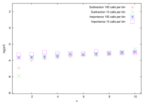
(a) Gaussian $m=10$

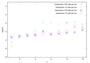
(b) Gaussian $m=100$

Figure 5: Log of the standard error over the integral evaluation for equation (19) versus dimension using $4\times 10^{4}$ points on the grid obtained after four iterations of $4\times 10^{4}$ calls. (a) $m=10$ the subtraction method works well in low dimensions. (b) $m=100$ for this many function calls the subtraction method breaks down in dimension greater than $5$ the separate integral estimates are inconsistent with large $\chi^{2}$ and the error is large. In contrast, importance sampling works well here.

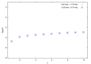
(a) Gaussian $m=10$

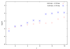
(b) Gaussian $m=100$

Figure 6: Log of the standard error over the integral evaluation for equation (19) versus dimension using $4\times 10^{4}$ points on the grid obtained after four iterations of $4\times 10^{4}$ calls. For both cases the mixed approach works well, retaining the advantage of subtraction in low dimensions and the stability of importance sampling in high. Calls per bin = $100$.

The integral

$$\int_{[0,1]^{d}}dx_{1}\cdots dx_{d}\prod_{i}^{n}\sqrt{\frac{m}{\pi}}\exp\left(-m(x_{i}-{\mathchoice{\textstyle{1\over 2}}{\scriptstyle{1\over 2}}{\scriptscriptstyle{1\over 2}}{1/2}})^{2}\right)=\left[\mathop{\rm erf}\left(\frac{\sqrt{m}}{2}\right)\right]^{d}$$ (19)

is another interesting case. When the parameter $m$ is small, the Gaussian is broad and our integration scheme approximates the true value well. However as the dimension increases our method fails to find the peak of the Gaussian as well as VEGAS and the integration starts to break down. The subtraction method can be improved by increasing the number of points per bin, however it still does slightly worse than VEGAS. This is possibly due to the interpolation performed during the rebinning step failing to reconstruct the approximation function. There is no reason for subtraction to be better in this case and we find, for a fixed number of calls as the dimension increases and therefore, the number of bins per axis reduces for this function subtraction gets worse more quickly than importance sampling.

Importance sampling will do better than subtraction in some cases and vice versa therefore combining the two approaches may be beneficial. We can do subtraction for some percentage of our total number of function evaluations, generating an approximation function and then do importance sampling on $f-\hat{f}$ for the remainder. Or we could do an initial run of importance sampling, then construct the approximation function on the bins with width given by $\rho$. Figure 6 shows the integral (19) in various dimensions using both varieties of mixed sampling. The mixed sampling is done by using $25\%$ of the function evaluations on one kind of sampling and then using the grid and approximation function found this way for the rest of the calls. The mixed strategies seem to give good results reproducing the superiority of subtraction in low dimensions and the stability of importance sampling in higher.

As an interesting practical example we perform the integral derived from the Feynman parameterization of the scalar Feynman diagram shown in Figure 7 in $4$-dimensional Euclidean space, and given explicitly in a file attached to this paper.

Figure 7: $\phi^{3}$ theory graph evaluated in the text. Explicitly given in attached files.

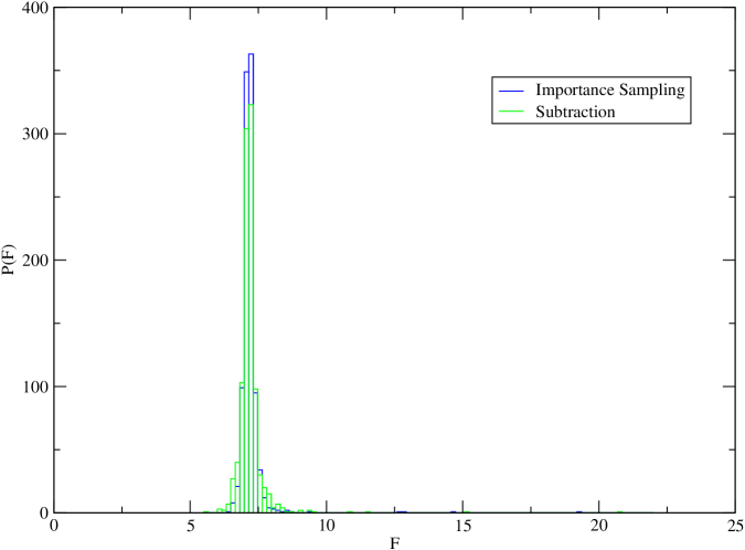
Figure 8: Distribution of results for the $\phi^{3}$ graph. The distribution is non-Gaussian in both cases with values differing significantly from the mean occuring far more often than if it were Gaussian — the “fat tail” of the distribution.

This integral is known to converge (its exact value is $-7.2123414\ldots$) but it is not necessarily square integrable and its higher moments may not exist. We plot the distribution obtained from evaluating the integral $1,000$ times by subtraction and importance sampling. The distribution looks distinctly non-Gaussian. It is peaked around the exact value but were the standard deviation used to estimate the error it would be incorrect. This kind of problem with parameter integrals arises often in practice and we advise caution in interpreting the output of any Monte Carlo calculation.

6 Conclusions

We have reviewed Monte Carlo integration, pointing out some often overlooked issues when the integral exists but the variance or some higher moments do not. This leads to non-Gaussian distributions and inaccurate estimates of the error. We have proposed a new algorithm for numerical Monte Carlo integration based on adaptive subtraction. We expect this method to have an advantage over importance sampling Monte Carlo schemes for some integrands. We have implemented our proposed adaptive subtraction method and found it to be better than importance sampling in some cases. A combination of the two methods can be better than either separately. We have given an explicit program, PANIC which is competitive with VEGAS. PANIC also shares the assumption of factorisability into a product of functions with VEGAS, thus improvements to VEGAS that work around this assumption, e.g., [5, 8], will also work with subtraction and are an interesting future direction. The subtraction idea can work with any Monte Carlo scheme and the subtraction function can even be constructed independently, in this paper we have seen good results when combined with importance sampling. Our code, PANIC, is included.

References

- [1] Rick Durrett, “Probability Theory and Examples”, (4th Edition), Cambridge, 2010. ISBN 9780521765398.
- [2] F. James, Rept. Prog. Phys. 43 (1980) 1145.
- [3] J M Hammersley and D. C. Handscomb, “Monte Carlo Methods”, Methuen, London, 1964.
- [4] G. P. Lepage, J. Comput. Phys. 27 (1978) 192.
- [5] T. Ohl, Comput. Phys. Commun. 120 (1999) 13 [hep-ph/9806432].
- [6] W.H. Press and G.R. Farrar, Computers in Physics, v4 (1990), pp. 190-195.
- [7] http://www.gnu.org/software/gsl/
- [8] T. Hahn, Comput. Phys. Commun. 168 (2005) 78 [hep-ph/0404043].
- [9] B. Lautrup Proceedings of the Colloquium on Computational Physics, Marseille, 1–57, 1971, (unpublished).