Invariant Generation through Strategy Iteration in Succinctly Represented Control Flow Graphs

Abstract.

We consider the problem of computing numerical invariants of programs, for instance bounds on the values of numerical program variables. More specifically, we study the problem of performing static analysis by abstract interpretation using template linear constraint domains. Such invariants can be obtained by Kleene iterations that are, in order to guarantee termination, accelerated by widening operators. In many cases, however, applying this form of extrapolation leads to invariants that are weaker than the strongest inductive invariant that can be expressed within the abstract domain in use. Another well-known source of imprecision of traditional abstract interpretation techniques stems from their use of join operators at merge nodes in the control flow graph. The mentioned weaknesses may prevent these methods from proving safety properties.

The technique we develop in this article addresses both of these issues: contrary to Kleene iterations accelerated by widening operators, it is guaranteed to yield the strongest inductive invariant that can be expressed within the template linear constraint domain in use. It also eschews join operators by distinguishing all paths of loop-free code segments. Formally speaking, our technique computes the least fixpoint within a given template linear constraint domain of a transition relation that is succinctly expressed as an existentially quantified linear real arithmetic formula.

In contrast to previously published techniques that rely on quantifier elimination, our algorithm is proved to have optimal complexity: we prove that the decision problem associated with our fixpoint problem is $\mathsf{\Pi^{p}_{2}}$-complete. Our procedure mimics a $\mathsf{\Pi^{p}_{2}}$ search.

1. Introduction

Static program analysis aims at deriving properties that are valid for all possible executions of a program, through an algorithmic processing of its source or object code. Examples of interesting properties include: “the program always terminates”; “the program never executes a division by zero”; “the program never dereferences a null pointer”; “the value of variable x always lies between 1 and 3”; “the output of the program is well-formed XHTML”. There is considerable practical interest in being able to prove such properties automatically, in particular for software used in safety-critical applications, e.g., in fly-by-wire flight control systems in aircraft [60].

1.1. Abstract interpretation

It is well-known that fully automatic, sound and complete program analysis is impossible for any nontrivial property regarding the final output of a program. All analysis methods therefore suffer from at least one of the following limitations: they may be limited to programs with finite (and not too large) memory, or to bounded execution times; they may be unsound (they may infer untrue properties); or they may be incomplete (they fail to prove certain true properties). In this article, we use the abstract interpretation framework of Cousot and Cousot [18] to construct a static analysis technique that is sound, but incomplete.

Static analysis by abstract interpretation replaces the computation over concrete reachable states by computations over symbolically represented sets of concrete states. The sets are taken from an abstract domain. For instance, one may aim at computing, for each program point $p$ and each program variable $x$, an interval in which the value of $x$ is guaranteed to lie whenever the program reaches program point $p$. An analysis solely based on such intervals is known as interval analysis [17]. More refined numerical analyses include, for instance, finding for each program point an enclosing polyhedron for the vector of program variables [19]. By restricting the analysis to handle only sets found within a particular abstract domain (e.g., Cartesian products of intervals or convex polyhedra), one can make the problem tractable, at the expense of over-approximation. For instance, if the domain in use consists of convex shapes, only, non-convex invariants will necessarily get over-approximated.

In addition to the abstract domain not being able to represent the required properties, a major source of imprecision is the use of widening operators to enforce the convergence of Kleene iterations within finitely many iteration steps [18]. These operators extrapolate the first iterates of the Kleene sequence, say, of the intervals $[0,1]$, $[0,2]$, $[0,3]$, $\dots$ to a plausible limit, say $[0,+\infty)$, ensuring termination of the accelerated iteration. However, such an accelerated iteration may overshoot the target, leading to further over-approximations of the desired result. In order to regain precision lost by widening, one can then apply narrowing. In its simplest form, narrowing is a descending iteration towards a fixpoint that strengthens the invariant step by step. For more detailed information on Kleene iteration techniques in the context of abstract interpretation, we refer the reader to Cousot and Cousot [18]. Many variants of this basic iteration scheme have been proposed to alleviate the over-approximations introduced by widening [35, 34, 38]. However, all these techniques do not guarantee to find the strongest inductive invariant that can be expressed in the abstract domain in use.

Let us illustrate the above mentioned weaknesses on the following simple example:

⬇

i = 0;

while (true) {

if (i < 10) i = i+2;

else goto _end; }

_end: printf(”i␣=␣%d\n”);

The strongest invariant, that is, the set of reachable states, is given by the proposition $i\in\{0,2,4,6,8,10\}$, which, together with the exit condition $i\geq 10$, yields $i=10$ as the only possible final value of $i$ at program point _end. Interval analysis by Kleene iterations with widenings computes the intervals $[0,0],[0,2],[0,4]$ and may then widen to $[0,+\infty)$. The narrowing phase yields the inductive invariant $i\in[0,11]$. From this we can conclude that the final value of $i$ is in the interval $[10,11]$. The obtained interval $[0,11]$ represents the strongest inductive invariant that can be expressed as an interval. It is, however, not the strongest invariant expressible as an interval, which is $i\in[0,10]$. The invariant $i\in[0,10]$ is not inductive, because a state with $i=9$ is mapped to a state with $i=11$ by one iteration of the loop.

Unfortunately, small changes to the above program can make the widening/narrowing approach fail to produce a good invariant. Consider, for instance, the introduction of an additional non-deterministic choice, represented by the function choice():

⬇

i = 0;

while (true) {

if (choice()) {

if (i < 10) i = i+2;

else goto _end; } }

_end: printf(”i␣=␣%d\n”);

The program still outputs the value $10$, whenever it terminates. The only difference from the first version of the program is that there is, in each iteration, a non-deterministic choice whether or not the original loop body is to be executed. If we perform the widening/narrowing technique on the modified version, the widening phase will produce the same result $[0,+\infty)$. However, the narrowing phase is now not able to regain any precision lost due to widening. The loop body represents the relation $\tau=\{(i,i)\mid i\in\mathbb{Z}\}\cup\{(i,i+2)\mid i\in\mathbb{Z}\text{ and }i<10\}$. This relation is reflexive, that is, $(i,i)\in\tau$ for all $i\in\mathbb{Z}$. The problem is of a general nature: Whenever the transition relation $\tau$ of a loop is reflexive, descending iterations fail to improve the inductive invariant obtained by widening.

Of course, on such a simple example, one could use simple tricks to get rid of the imprecision and recover the interval $[0,11]$: remove the identity from the transition relation (this does not change the set of all (inductive) invariants), or try a form of widening with thresholds, also known as widening “up to” [39]. However, such approaches are brittle and may fail for more complex programs.

1.2. Alternatives to the widening/narrowing approach

Because of the known weaknesses of the widening/narrowing approach, alternative methods have been proposed. Finding an inductive invariant in an abstract domain can be recast as solving a constraint system. Finding the strongest inductive invariant is then the problem of finding a minimal solution to the constraint system. The technique described in this article is related to two recently proposed approaches, which we shall now briefly describe.

1.2.1. Quantifier elimination

Monniaux [48] considers abstract domains where elements are defined by a logical formula $I$ (more specifically, a conjunction of linear inequalities) that links the program variables to some parameters. For instance, intervals on two variables $x,y$ are defined by $I\operatorname{{}\mathrel{\mathop{:}}={}}-l_{x}\leq x\leq u_{x}\land-l_{y}\leq y\leq u_{y}$, where $l_{x},u_{x},l_{y},u_{y}$ are the parameters. An element from the abstract domain defined by the template $I$ is specified by an assignment of values to the parameters.

Consider a set of initial states given by a formula $\iota$ (in the above example, with free variables $\sigma=(x,y)$) and a transition relation given by $\tau$ (in the above example, with free variables $(\sigma,\sigma^{\prime})=(x,y,x^{\prime},y^{\prime})$). $I$ defines an inductive invariant for $\iota$ and $\tau$ if and only if

$$\forall\sigma\,.\,\iota(\sigma)\Rightarrow I(\sigma)\land\forall\sigma,\sigma^{\prime}\,.\,\left(I(\sigma)\land\tau(\sigma,\sigma^{\prime})\Rightarrow I(\sigma^{\prime})\right).$$ (1)

Here, $I(\sigma)$ is the formula $I$ as above and $I(\sigma^{\prime})$ is the formula $I$ with $\sigma$ replaced by $\sigma^{\prime}$. The free variables of formula (1) are the parameters in $I$. In the above example, they are $l_{x},u_{x},l_{y},u_{y}$. Any satisfying assignment to these variables defines an inductive invariant from the abstract domain. A least inductive invariant in the abstract domain is then defined by constructing, using formula (1) as a building block, a formula whose solution is the minimal solution of (1), using that, for any formula $F$, $x_{0}=\min\{x\mid F(x)\}$ if and only if

$$F(x_{0})\land\forall x\,.\,\left(F(x)\Rightarrow x_{0}\leq x\right).$$ (2)

The static analyzer then proceeds as follows: transform the loop into a set of initial states $\iota$ and a transition relation $\tau$. From these formulas, construct Formula 2. Then, call a solver capable of dealing with quantified formulas, e.g, a quantifier elimination procedure or a lazy version thereof such as the one developed by Monniaux [47].

As an extension to this framework, $\iota$ and $\tau$ may have additional variables, e.g., precondition or system parameters. The formula defining the least inductive invariant will then take the invariant parameters as a partial function (in the mathematical sense, that is, as a binary related each input to at most one output) of these precondition or system parameters. By quantifier elimination and further processing of the formula, it is possible to turn this formula into a closed-form function, and even into executable code computing that function (a tree of if-then-else statements with assignments at the leaves).

This approach allows to effectively synthesize best abstract transformers ($\alpha\circ\tau\circ\gamma$ in the notation of Cousot and Cousot [18]). Unfortunately, quantifier elimination over linear real arithmetic is still very costly, despite the various recent works on this problem, and quantifier elimination over linear integer arithmetic and polynomial real arithmetic are even costlier.

The technique described in this article considers the same problem as the quantifier elimination approach, but without preconditions or system parameters. Our technique also uses a different algorithmic approach, called max-strategy iteration.

1.2.2. Strategy Iteration

In this article, we introduce a refinement of the max-strategy iteration technique of Gawlitza and Seidl [26] for template linear constraint domains. The phrase “strategy iteration”, also known as “policy iteration”, comes from game theory. Let us consider two-players zero-sum games: the outcome of such a game is a real number, the two players (the maximizer and the minimizer) aim at maximizing (respectively, minimizing) the outcome. Strategy iteration is a method for computing the optimal strategy for one of the players. It successively improves a strategy through the following two steps until an optimal strategy is found: (Evaluation) Evaluate the currently selected strategy; and (Improvement) try to improve the currently selected strategy w.r.t. the result of the evaluation.

The max-strategy iteration technique of Gawlitza and Seidl [26] for finding invariants is inspired by this game-theoretic approach. Instantiated on template linear constraint domains, it computes the strongest inductive invariant that can be represented by polyhedra of the form $P(b)=\{x\in\mathbb{R}^{n}\mid Tx\leq b\}$, where $T\in\mathbb{R}^{m\times n}$ is a template constraint matrix, which is fixed before the analysis is run (heuristics for finding a suitable matrix are out-of-scope for this article). The variable $x$ is the vector of program variables. The template constraint matrix $T$ is the counterpart of the template $I$ from the quantifier elimination technique of Monniaux [48]. Given $T$, every vector $b\in{\overline{\mathbb{R}}}^{m}$ uniquely determines a polyhedron $P(b)$. The vector $b$ contains the bounds on the linear functions that are represented by the rows of $T$. With the appropriate choice of $T$ we can, among others, express the popular interval [17] and octagon [46, 45] abstract domains.

Similarly to Kleene iterations, the max-strategy improvement algorithm produces an ascending sequence of pre-fixpoints that are less than or equal to the least inductive invariant we are aiming for. The pre-fixpoints are obtained through convex optimization techniques, e.g., linear programming. In contrast to Kleene iterations, though, the algorithm converges to the least inductive invariant after at most exponentially many steps. Our conjecture is that it usually converges fast in practice, though one can concoct artificial examples that exhibit exponential behavior.

1.2.3. Trace partitioning

Max-strategy iteration rids us of imprecisions introduced by widening, but, per se, does not remove imprecisions introduced by another operation: the merging of information from different program paths at join nodes in the control flow graph. In this article, we introduce a refinement of max-strategy iteration where we distinguish the various execution paths, in a manner similar to the work of Monniaux [48], and Monniaux and Gonnord [49].

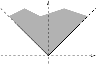
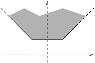
Figure 1. On the left: the graph of $y=|x|$ is the union of two half-lines, but computing their convex hull yields the grayed shape. By intersection with $y\geq 1$, we obtain the shape on the right, which contains points with $x=0$ even though $y=|x|\land y\geq 1$ has no solution with $x=0$.

In most systems for static analysis by abstract interpretation, joins in the control-flow graph result in computations of least upper bounds in the abstract domain. For instance, consider abstract interpretation over general convex polyhedra on the following program:

⬇

if (x >= 0) y = x;

else y = -x;

if (y >= 1) z = 3.5/x;

The program divides $3.5$ by the value of x provided that the absolute value of x is at least $1$. A static analyzer that uses convex polyhedra as abstract domain may work as follows. After the first if-then-else statement, a convex hull is computed between the $x\geq 0\land y=x$ and $x<0\land y=-x$ half-lines, resulting in a much larger polyhedron (see Fig. 1). The imprecision introduced by this operation prevents the analyzer from proving that a division by zero at line $3$ is impossible.

Figure 2. Instead of considering two transitions (corresponding to a first if-then-else) followed by convex hull followed by two transitions (corresponding to a second if-then-else), as on the left, we get better precision by considering the four product transitions, as on the right.

One solution is to get rid of all convex hulls corresponding to control flow joins by removing all control flow joins, except those corresponding to loop headers, by combining control flow edges. For instance, $n$ successive if-then-else constructs can be turned into an expanded system of $2^{n}$ transitions (Figure 2 shows this construction for $n=2$). This is close to the trace partitioning approach of Rival and Mauborgne [53]. One could therefore run this exponential transformation first, and then run max-strategy iteration or min-strategy iteration (Sec. 1.4). However, this transformation causes an exponential blowup and is therefore clearly not scalable.

In this article, we describe an algorithm that yields the same result as max-strategy iteration on this exponentially larger system. Our algorithm uses only polynomial space. It achieves this by keeping the exponentially large system implicit.

1.2.4. Path focusing

Monniaux and Gonnord [49], Henry et al. [40] propose to run the classical Kleene iterations with widening and narrowing scheme not on the original control-flow graph, but on this exponentially larger system. In this approach, iterations are run on a distinguished subset of the original control nodes, such that all cycles in the original control flow graphs cross at least one of these distinguished nodes, using transitions corresponding to the simple paths between these distinguished nodes in the original control flow graph. The expanded control multigraph is kept implicit: the transitions, corresponding to simple paths in the original graph, are obtained on demand as solutions to SMT problems. This approach has the following advantages:

1. It fully does away with imprecisions introduced by “join” operations, except those corresponding to loops.

2. The transition relations on the simple paths may be accelerable. That is, they can be dealt with through acceleration techniques (cf. Sec. 1.4, [33, 32, 43]).

3. While it uses widening operators, it does away with some of the imprecisions they introduce by focusing on one path at a time, which allows the use of narrowing iterations even on programs where they fail to yield better precision with the classical iteration scheme.

The technique we present in this article combines the idea of implicit representation with max-strategy iteration.

1.3. Contributions

The main contribution of this article is an algorithm that computes the strongest inductive invariant of the expanded transition system (which allows higher precision for abstract interpretation) without actually constructing it. We shall see later the exact definition, but here is an interesting particular case (the general result allows more complex control flow): given a $m\times n$ matrix $A$, an initial value $\iota\in\mathbb{Q}^{n}$ and a transition relation $\tau$ over $\mathbb{Q}^{n}$, defined by a formula over variables $x_{1},\dots,x_{n},x^{\prime}_{1},\dots,x^{\prime}_{n}$, built with non-strict linear (in)equalities, $\land$, $\lor$ and prenex $\exists$, compute the least set of the form $P(b)=\{x\in\mathbb{R}^{n}\mid Ax\leq b\}$ (that is, compute $b$) containing $\iota$ and stable by the transition relation $\tau$; equivalently, find the least loop invariant of the form $Ax\leq b$ for the loop with initial state $\iota$ and loop body expressed by $\tau$.

Our algorithm can be performed in polynomial space and exponential time. It works in a demand-driven fashion: elements from the exponentially-sized sets of strategies and loop-free paths are enumerated only as needed, and one can thus hope that they will not all be enumerated, which seems to be confirmed by our preliminary experiments.

We also consider the following associated decision problem, which we shall later make more formal:

“Given a control-flow graph (with $N$ vertices) and transition relations written as existentially quantified first-order linear real arithmetic formulas, a family $A_{1},\dots,A_{N}$ of matrices, an initial control state and a “bad” control state $b$, does there exist vectors $b_{1},\dots,b_{N}$ such that $A_{1}x\leq b_{1}\land\dots\land A_{N}x\leq b_{N}$ forms an inductive invariant proving that $b$ is unreachable?”.

We show this problem to be $\mathsf{\Sigma^{p}_{2}}$-complete (at the second level of the polynomial time hierarchy [50, ch. 17]), even if $N=1$ and the matrix is $1\times 1$. Equivalently, the negated problem (abstract reachability of a statement) is shown to be $\mathsf{\Pi^{p}_{2}}$-complete. Assuming the polynomial hierarchy does not collapse, this mean that this problem can be solved in polynomial space, but is harder than NP-complete and coNP-complete problems. This clearly justifies the use of an exponential-time algorithm.

1.4. Other related Work

Many approaches have been proposed to address the imprecisions caused by widening operators. We now briefly describe approaches related to ours, in addition to those that we directly build upon (Sec. 1.2). Halbwachs et al. [39] proposed widening “up to” (an idea resurrected in the Astrée system as widening with thresholds [8, 9]), which extracts syntactic hints for limiting widening. Bagnara et al. [4, 5] proposed improvements over the “classical” widenings on linear constraint domains [37]. Gopan and Reps [34] introduced “look-ahead widening” [34] and “guided iterations” [35]: standard widening-based analysis is applied to a sequence of syntactic restrictions of the original program, which ultimately converges to the whole program; the idea is to distinguish phases or modes of operation in order to make the widening more precise. Some other techniques fully do away with widenings [13, 15, 55], for instance by expressing the invariants as solutions of a mathematical programming problem [36], and thus the least invariant in the domain as an optimal solution to this problem.

In some cases, it is possible to compute exactly the transitive closure of the transition relation, or the application of the transitive closure to given initial states, or at least to compute a good over-approximation thereof. Such acceleration techniques [33, 32, 43] tend to have difficulties dealing with programs where the control flow is not flat (multiple paths within the loop body).

In Section 1.2.2, we sketched max-strategy iteration by an analogy to solving games where “max” operations correspond to control-flow joins and “min” operations to guards. If instead of choosing arguments to “max” operators, the strategy chooses them for “min” operators, we obtain min-strategy iteration [14, 24]. Min-strategy iteration solves a sequence of fixpoint problems with decreasing values always weaker or equivalent to the strongest inductive invariant in the domain. In general, this sequence does not necessarily converge to this least inductive invariant, but it does so under certain conditions (e.g., when all abstract transformers are non-expansive [1]). We investigated applying our “implicit representation” idea to the min-strategy approach, but encountered a stumbling block: while it is possible to decide whether a max-strategy is improvable using SMT solving on quantifier-free formulas, the equivalent for min-strategies necessitated quantified formulas, which defeats the purpose of doing away with quantifier elimination techniques.

2. Basics

2.1. Notations

$\mathbb{B}=\{0,1\}$ denotes the set of Boolean values. The set of real numbers (resp. the set of rational numbers) is denoted by $\mathbb{R}$ (resp. $\mathbb{Q}$). The complete linearly ordered set $\mathbb{R}\cup\{{{-}\infty},\infty\}$ is denoted by ${\overline{\mathbb{R}}}$, similarly $\mathbb{Q}\cup\{{{-}\infty},\infty\}$ is denoted by $\overline{\mathbb{Q}}$. For any expression (resp. term) $e$, we write $e[e_{1}/{\bf x}_{1},\ldots,e_{k}/{\bf x}_{k}]$ to denote the expression (resp.  term) that is obtained from $e$ by simultaneously replacing all occurrences of the variables ${\bf x}_{1}$, …, ${\bf x}_{k}$ by $e_{1},\ldots,e_{k}$.

A partially ordered set $\mathbb{D}$ is called a lattice if and only if any two elements $x,y\in\mathbb{D}$ have a greatest lower bound and a least upper bound, denoted respectively by $x\wedge y$ and $x\vee y$. It is a complete lattice if and only if any subset $X\subseteq\mathbb{D}$ has a greatest lower bound and a least upper bound, denoted by $\bigwedge X$ and $\bigvee X$. The least element $\bigvee\emptyset$ of a complete lattice is denoted by $\bot$. The greatest element $\bigwedge\emptyset$ is denoted by $\top$.

Assume that $\mathbb{D}_{1}$ and $\mathbb{D}_{2}$ are partially ordered by $\leq_{1}$ and $\leq_{2}$, respectively. A function $f:\mathbb{D}_{1}\rightarrow\mathbb{D}_{2}$ is called monotone if and only if $f(x)\leq_{2}f(y)$ for all $x,y\in\mathbb{D}_{1}$ with $x\leq_{1}y$. We shall often use the following fundamental result:

Theorem 1 (Knaster/Tarski [62]).

Let $\mathbb{D}$ be a complete lattice and $f:\mathbb{D}\rightarrow\mathbb{D}$ monotone. The operator $f$ has a least fixpoint and a greatest fixpoint, respectively denoted by $\mu f$ and $\nu f$. Moreover, we have $\mu f=\bigwedge\{x\in\mathbb{D}\mid f(x)\leq x\}$ and $\nu f=\bigvee\{x\in\mathbb{D}\mid x\leq f(x)\}$. ∎

We denote the transpose of a matrix $A$ by $A^{\top}$. For $x\in{\overline{\mathbb{R}}}$, we denote the column vector $(x,\ldots,x)^{\top}$ by $\underline{x}$. We denote the $i$-th row (resp. the $j$-th column) of a matrix $A$ by $A_{i\cdot}$ (resp. $A_{\cdot j}$). Accordingly, $A_{i\cdot j}$ denotes the entry in the $i$-th row and the $j$-th column. We also use this notation for vectors and mappings $f:X\to Y^{k}$, i.e., for all $i\in\{1,\cdots,k\}$, the mapping $f_{i\cdot}:X\to Y$ is given by $f_{i\cdot}(x)=(f(x))_{i\cdot}$ for all $x\in X$. The set ${\overline{\mathbb{R}}}^{n}$ is partially ordered by the component-wise extension of $\leq$, which we again denote by $\leq$. That is, for all $x,y\in{\overline{\mathbb{R}}}^{n}$, $x\leq y$ if and only if $x_{i\cdot}\leq y_{i\cdot}$ for all $i\in\{1,\ldots,n\}$.

A mapping $f:{\overline{\mathbb{R}}}^{n}\to{\overline{\mathbb{R}}}^{m}$ is called affine if and only if there exist $A\in\mathbb{R}^{m\times n}$ and $b\in{\overline{\mathbb{R}}}^{m}$ such that $f(x)=Ax+b$ for all $x\in{\overline{\mathbb{R}}}^{n}$. Here, we use the convention ${{-}\infty}+\infty={{-}\infty}$. Observe that $f$ is monotone if all entries of $A$ are non-negative. A mapping $f:{\overline{\mathbb{R}}}^{n}\to{\overline{\mathbb{R}}}$ is called weak-affine if and only if there exist $a\in\mathbb{R}^{n}$ and $b\in{\overline{\mathbb{R}}}$ such that $f(x)=a^{\top}x+b$ for all $x\in{\overline{\mathbb{R}}}^{n}$ with $f(x)\neq{{-}\infty}$. A mapping $f:{\overline{\mathbb{R}}}^{n}\to{\overline{\mathbb{R}}}^{m}$ is called weak-affine if and only if there exist weak-affine mappings $f_{1},\ldots,f_{m}:{\overline{\mathbb{R}}}^{n}\to{\overline{\mathbb{R}}}$ such that $f=(f_{1},\ldots,f_{m})^{\top}$. Every affine mapping is weak-affine, but not vice-versa. In this article, we are concerned with mappings that are point-wise minimums of finitely many monotone and weak-affine mappings. Note that these mappings are in particular concave, i.e., the set of points below the graph of the function is convex.

2.2. Linear Programming

Linear programming aims at optimizing a linear objective function with respect to linear constraints. In this article, we consider linear programming problems (LP problems for short) of the form $\sup\,\{c^{\top}x\mid x\in\mathbb{R}^{n},Ax\leq b\}$. Here, $A\in\mathbb{R}^{m\times n}$, $b\in\mathbb{R}^{m}$, and $c\in\mathbb{R}^{n}$ are the inputs. The convex closed polyhedron $\{x\in\mathbb{R}^{n}\mid Ax\leq b\}$ is called the feasible space. The LP problem is called infeasible if and only if the feasible space is empty. An element of the feasible space, is called feasible solution. A feasible solution $x$ that maximizes $c^{\top}x$ is called optimal solution.

If $A$ and $b$ consist of rational entries, only, then the feasible space is nonempty if and only if it contains a rational point. An optimal solution exists if and only if there exists a rational one. In this article, we always assume that all numbers in the input are rational.

LP problems can be solved in polynomial time through the ellipsoid method [41] and interior point methods [57]. However, the running-time of these algorithms crucially depends on the sizes of occurring numbers. At the danger of an exponential running-time in contrived cases, we can also instead rely on the simplex algorithm: its worst-case running-time does not depend on the sizes of occurring numbers (given that arithmetic operations, comparison, storage and retrieval for numbers are counted for $\mathcal{O}(1)$). See for example Schrijver [57], Dantzig [20] for more information on linear programming.

2.3. SAT modulo linear real arithmetic

The set of SAT modulo linear real arithmetic formulas $\Phi$ is defined through the following grammar:

$$e ::=c\mid x\mid e_{1}+e_{2}\mid c\cdot e^{\prime} \Phi ::=a\mid e_{1}\leq e_{2}\mid e_{1}<e_{2}\mid\Phi_{1}\vee\Phi_{2}\mid\Phi_{1}\wedge\Phi_{2}\mid\neg\Phi^{\prime}$$ (3)

Here, $c\in\mathbb{Q}$ is a constant, $x$ is a real valued variable, $e,e^{\prime},e_{1},e_{2}$ are real-valued linear expressions, $a$ is a Boolean variable and $\Phi,\Phi^{\prime},\Phi_{1},\Phi_{2}$ are formulas. An interpretation $I$ for a formula $\Phi$ is a mapping that assigns a real value to every real-valued variable and a Boolean value to every Boolean variable. We write $I\models\Phi$ for “$I$ is a model of $\Phi$”. That is, we firstly inductively define a function $\llbracket e\rrbracket$ that evaluates a linear expression $e$ as follows:

$$\llbracket c\rrbracket I =c \llbracket x\rrbracket I =I(x) \llbracket e_{1}+e_{2}\rrbracket I =\llbracket e_{1}\rrbracket I+\llbracket e_{2}\rrbracket I \llbracket c\cdot e^{\prime}\rrbracket I =c\cdot\llbracket e^{\prime}\rrbracket I$$ (4)

Secondly, we inductively define the relation $\models$ as follows:

$$I\models a \iff I(a)=1 I\models e_{1}\leq e_{2} \iff\llbracket e_{1}\rrbracket I\leq\llbracket e_{2}\rrbracket I$$

$$I\models e_{1}<e_{2} \iff\llbracket e_{1}\rrbracket I<\llbracket e_{2}\rrbracket I I\models\Phi_{1}\vee\Phi_{2} \iff I\models\Phi_{1}\text{ or }I\models\Phi_{2}$$ (5)

$$I\models\Phi_{1}\wedge\Phi_{2} \iff I\models\Phi_{1}\text{ and }I\models\Phi_{2} I\models\neg\Phi^{\prime} \iff I\not\models\Phi^{\prime}$$

A formula is called satisfiable if and only if it has at least one model. A formula has a model if and only if it has a rational model.

The problem of deciding the satisfiability of SAT modulo linear real arithmetic formulas is NP-complete. There nevertheless exist efficient solver implementations for this decision problem, generally based on the DPLL(T) approach, an extension of the DPLL algorithm for SAT to richer logics. For more information see for example Biere et al. [7], Dutertre and de Moura [22], and Kroening and Strichman [42]. Such implementations, on satisfiable instances, can provide a model over Booleans and rational numbers.

In order to simplify notations we also allow matrices, vectors, the relations $\geq,\allowbreak>,\allowbreak\neq,\allowbreak=$, and the Boolean constants $0$ and $1$ to occur in SAT modulo linear real arithmetic formulas.

3. The Framework

3.1. Control Flow Graphs and Collecting Semantics

In this article, we model programs as control flow graphs, i.e., a program $G$ is a triple $(N,E,{\bf st})$, where

1. $N$ is a finite set of program points,

2. $E\subseteq N\times{\bf Stmt}\times N$ is a finite set of control-flow edges, and

3. ${\bf st}\in N$ is the start program point.

A program uses $n$ real-valued variables ${\bf x}_{1},\ldots,{\bf x}_{n}$. A state is described by a vector $x\in\mathbb{R}^{n}$. We assign a collecting semantics $\llbracket s\rrbracket:2^{\mathbb{R}^{n}}\to 2^{\mathbb{R}^{n}}$ to each statement $s\in{\bf Stmt}$. The collecting semantics $\llbracket s\rrbracket$ is an operator that assigns a set $\llbracket s\rrbracket(X)$ of possible states after the execution of $s$ to a set $X$ of possible states before the execution of $s$. The set ${\bf Stmt}$ of statements is specified subsequently. The collecting semantics $V$ of a program $G=(N,E,{\bf st})$ is finally defined as the least solution of the following constraint system:

$${\bf V}[{\bf st}] \supseteq\mathbb{R}^{n} {\bf V}[v]\supseteq\llbracket s\rrbracket({\bf V}[u])\quad\text{for all }(u,s,v)\in E.$$ (6)

Here, for any $v\in N$, the variable ${\bf V}[v]$ takes values in $2^{\mathbb{R}^{n}}$. The components of the collecting semantics $V$ are denoted by $V[v]$ for all $v\in N$. Throughout this article, we will usually denote variables in bold face, and values in normal face.

3.2. Statements

The set ${\bf Stmt}$ of all statements is the set of all SAT modulo linear real arithmetic formulas without Boolean variables and without negation. Note that non-strict and strict inequality constraints are permitted. The formula $e_{1}\neq e_{2}$ is also permitted, since it is an abbreviation for $e_{1}<e_{2}\vee e_{2}<e_{1}$. We can (in linear time) transform any SAT modulo linear real arithmetic formula without Boolean variables into this form by pushing negations to the leaves.

The $\mathbb{R}$-valued variables ${\bf x}_{1},\ldots,{\bf x}_{n}$ and ${\bf x}_{1}^{\prime},\ldots,{\bf x}_{n}^{\prime}$, that may occur in the formula, play a particular role. The values of the variables ${\bf x}_{1},\ldots,{\bf x}_{n}$ represent the values of the program variables before executing the statement, and the values of the variables ${\bf x}_{1}^{\prime},\ldots,{\bf x}_{n}^{\prime}$ represent the values of the program variables after executing the statement. For convenience, we denote the vectors $({\bf x}_{1},\ldots,{\bf x}_{n})^{\top}$ and $({\bf x}_{1}^{\prime},\ldots,{\bf x}_{n}^{\prime})^{\top}$ also by ${\bf x}$ and ${\bf x}^{\prime}$, respectively. In addition to ${\bf x}_{1},\ldots,{\bf x}_{n}$ and ${\bf x}_{1}^{\prime},\ldots,{\bf x}_{n}^{\prime}$, the statement may also include other variables, which may stand for intermediate values computed (or non-deterministically chosen) during the execution of a program statement. Conceptually, these variables are existentially quantified.

We could also add Boolean variables, at the expense of some additional complexity in definitions, theorems and proofs. Note that this would not increase the expressiveness, since a Boolean variable ${\bf y}$ can be simulated by a real variable $\widetilde{{\bf y}}$ by replacing all occurrences of ${\bf y}$ by $\widetilde{{\bf y}}=1$, all occurrences of $\neg{\bf y}$ by $\widetilde{{\bf y}}=0$, and conjoining $(\widetilde{{\bf y}}=0\lor\widetilde{{\bf y}}=1$) to the formula. In practice, the direct support of Boolean variables may be beneficial for the efficiency. More generally, we can accommodate any formula feature that just expresses disjunctions in a compact way; the only requirement is not to generate negations.

The collecting semantics $\llbracket s\rrbracket:2^{\mathbb{R}^{n}}\to 2^{\mathbb{R}^{n}}$ of a statement $s\in{\bf Stmt}$ is defined by

$$\llbracket s\rrbracket(X) :=\{x^{\prime}\in\mathbb{R}^{n}\mid\exists x\in X\,.\,s[x/{\bf x},x^{\prime}/{\bf x}^{\prime}]\text{ is satisfiable}\} \text{for all }X\subseteq\mathbb{R}^{n}.$$ (7)

Consider the following C-code snippet:

⬇

if (x_1 >= 0)

x_2 = x_1;

else

x_2 = -x_1;

Assume that x_1 and x_2 are of type int and that they are the only numerical variables. The effect of the C code snippet can be abstracted by the statement

$${\bf x}_{1}^{\prime}={\bf x}_{1}\wedge\left(\left({\bf x}_{1}\geq 0\wedge{\bf x}_{2}^{\prime}={\bf x}_{1}\right)\vee\left({\bf x}_{1}<0\wedge{\bf x}_{2}^{\prime}=-{\bf x}_{1}\right)\right)$$ (8)

Note that a conjunct ${\bf x}^{\prime}_{i}={\bf x}_{i}$ is needed for all variables that do not change their values.

A statement $s$ is called merge-simple if and only if it is in disjunctive normal form, i.e., $s$ is of the form $s_{1}\vee\cdots\vee s_{k}$, where the statements $s_{1},\ldots,s_{k}$ do not use the Boolean connector $\vee$. Any statement can be rewritten into an equivalent merge-simple statement in exponential time and space using distributivity. The crux of our main result is that our algorithm never needs to compute such an exponentially-sized disjunctive normal form.

If we convert Statement (8) into an equivalent merge-simple statement using distributivity, we get:

$$\left({\bf x}_{1}^{\prime}={\bf x}_{1}\wedge{\bf x}_{1}\geq 0\wedge{\bf x}_{2}^{\prime}={\bf x}_{1}\right)\vee\left({\bf x}_{1}^{\prime}={\bf x}_{1}\wedge{\bf x}_{1}<0\wedge{\bf x}_{2}^{\prime}=-{\bf x}_{1}\right)$$ (9)

A merge-simple statement $s$ that does not use the Boolean connector $\vee$ at all is called sequential. Intuitively, sequential statements correspond to straight-line sequences of basic blocks. The merge-simple statement (9) non-deterministically chooses between executing one of the following sequential statement:

$${\bf x}_{1}^{\prime} ={\bf x}_{1}\wedge{\bf x}_{1}\geq 0\wedge{\bf x}_{2}^{\prime}={\bf x}_{1} {\bf x}_{1}^{\prime} ={\bf x}_{1}\wedge{\bf x}_{1}<0\wedge{\bf x}_{2}^{\prime}=-{\bf x}_{1}$$ (10)

3.3. Abstract Semantics

Let $\mathbb{D}$ be a complete lattice (for instance the complete lattice of all $n$-dimensional closed real intervals). Assume that $\alpha:2^{\mathbb{R}^{n}}\to\mathbb{D}$ and $\gamma:\mathbb{D}\to 2^{\mathbb{R}^{n}}$ form a Galois connection, i.e., for all $X\subseteq\mathbb{R}^{n}$ and all $d\in\mathbb{D}$, $\alpha(X)\leq d$ if and only if $X\leq\gamma(d)$. The abstract semantics $\llbracket s\rrbracket^{\sharp}:\mathbb{D}\to\mathbb{D}$ of a statement $s$ is then defined by

$$\llbracket s\rrbracket^{\sharp}:=\alpha\circ\llbracket s\rrbracket\circ\gamma.$$ (11)

Remark that we have chosen to use the best abstract transformer, i.e., the most precise abstract semantics. All that was needed for soundness is that $\llbracket s\rrbracket\circ\gamma(d)\subseteq\gamma\circ\llbracket s\rrbracket^{\sharp}(d)$ for all $d\in\mathbb{D}$. Our choice of $\llbracket s\rrbracket^{\sharp}(d)$, however, is the most accurate sound value.

The abstract semantics $V^{\sharp}$ of a program $G=(N,E,{\bf st})$ is the least solution of the following constraint system:

$${\bf V}^{\sharp}[{\bf st}] \geq\alpha(\mathbb{R}^{n}) {\bf V}^{\sharp}[v]\geq\llbracket s\rrbracket^{\sharp}({\bf V}^{\sharp}[u])\quad\text{for all }(u,s,v)\in E$$ (12)

Here, for any $v\in N$, the variable ${\bf V}^{\sharp}[v]$ takes values in $\mathbb{D}$. The components of the abstract semantics $V^{\sharp}$ are denoted by $V^{\sharp}[v]$ for all $v\in N$. The abstraction is sound, i.e., the abstract semantics $V^{\sharp}$ safely over-approximates the collecting semantics $V$, i.e., $\gamma(V^{\sharp}[v])\supseteq V[v]$ for all $v\in N$.

3.4. Template Linear Constraints

In this article we restrict our considerations to template linear constraint domains as introduced by Sankaranarayanan et al. [56]. We assume that a template constraint matrix $T\in\mathbb{R}^{m\times n}$ is given. For technical convenience, we always assume w.l.o.g. that $m\geq 1$ and each row of $T$ contains at least one non-zero entry. The template linear constraint domain can be identified with the set ${\overline{\mathbb{R}}}^{m}$. As shown by Sankaranarayanan et al. [56], the abstraction $\alpha:2^{\mathbb{R}^{n}}\to{\overline{\mathbb{R}}}^{m}$ and the concretization $\gamma:{\overline{\mathbb{R}}}^{m}\to 2^{\mathbb{R}^{n}}$, which are defined by

$$\gamma(d) :=\{x\in\mathbb{R}^{n}\mid Tx\leq d\} \text{for all }d\in{\overline{\mathbb{R}}}^{m},\text{ and}$$ (13)

$$\alpha(X) :=\textstyle\bigwedge\{d\in\mathbb{D}\mid\gamma(d)\supseteq X\} \text{for all }X\subseteq\mathbb{R}^{n},$$ (14)

form a Galois connection.

The template linear constraint domains contain intervals, zones, and octagons [45, 46], with appropriate choices of the template constraint matrix $T$ [56]. For instance, if we have two variables $x$ and $y$, and we abstract each variable by an interval as $x\in[-l_{x},u_{x}]$ and $y\in[-l_{y},u_{y}]$, the vector $d$ is formed of $(l_{x},l_{y},u_{x},u_{y})$. Here, the matrix $T$ is given by:

$$T=\begin{pmatrix}-1&0\\ 0&-1\\ 1&0\\ 0&1\\ \end{pmatrix}$$

and thus the concretization expresses:

$$\gamma\begin{pmatrix}l_{x}\\ l_{y}\\ u_{x}\\ u_{y}\end{pmatrix}=\left\{\begin{pmatrix}x\\ y\\ \end{pmatrix}\mid x\in[-l_{x},u_{x}],\,y\in[-l_{y},u_{y}]\right\}=\left\{\begin{pmatrix}x\\ y\\ \end{pmatrix}\mid\begin{pmatrix}-1&0\\ 0&-1\\ 1&0\\ 0&1\\ \end{pmatrix}\begin{pmatrix}x\\ y\\ \end{pmatrix}\leq\begin{pmatrix}l_{x}\\ l_{y}\\ u_{x}\\ u_{y}\end{pmatrix}\right\}$$

While intervals, zones, and octagons are somewhat “obvious” choices, a common discussion with respect to template domains is how to find the templates, as opposed to the domain of convex polyhedra, where the convex hull and widening operations somewhat “discover” interesting directions in space. In this article, we shall assume that template matrices are given and refrain from discussing how they were obtained.

4. Improving the Precision of the Abstraction

Most abstract interpretation techniques consider a control-flow graph with transitions expressed as sequential statements only (see formal definition in Sec. 3.2), that is, composed of atomic guards and assignments. An if-then-else construct with simple constructs (e.g., assignments) in both branches is thus expressed as two sequential statements, and a sequence of two such if-then-else constructs (one from point $A$ to point $B$ and one from $B$ to $C$) is expressed as on the left of Figure 2: two sequential statements between $A$ and $B$, and two sequential statements between $B$ and $C$. As noted in the introduction (Sec. 1.2.3), abstract interpretation techniques usually abstract the set of reachable states at point $B$. This may result in spurious states being considered in the abstraction, which in turn may result in the analysis tool being unable to prove desirable properties.

In this article, we apply an idea that is very similar to the path focusing technique of Monniaux and Gonnord [49]. Given a program expressed as a control-flow graph with sequential statements on the edges, we first compute a feedback vertex set (a.k.a. cut-set) $S$, that is, a set of control nodes (the feedback vertexes) such that removing them cuts all cycles in the graph. Our original program is equivalent to a program where the only control nodes are those in the feedback vertex set, but edges carry arbitrary statements instead of sequential statements only (cf. Sec. 3.2). The results of program analyses on this new graph, at nodes from the feedback vertex set $S$, are sound invariants for the original program. If information is needed at other nodes, we can compute it from the information we have for the nodes from $S$.

Since methods for obtaining compact formulas expressing these statements from the original program have already been described in other publications [49], we do not explain them in detail. Instead, we provide an example.

Figure 3. The program $G_{1}$ of the running example

[Running Example] Throughout this article we use the following C-code snippet as a running example:

⬇

int x_1, x_2;

x_1 = 0;

while (x_1 <= 1000) {

x_2 = -x_1;

if (x_2 < 0) x_1 = -2 * x_1;

else x_1 = -x_1 + 1; }

This C-code snippet is abstracted through the program $G_{1}=(N_{1},E_{1},{\bf st})$ depict in Figure 3. However, it is not necessary to apply abstraction at every program point, i.e., to assign an abstract value to each program point. It suffices to apply abstraction at a vertex feedback set of $G_{1}$. Since all loops contain the program point $1$, $\{1\}$ is a feedback vertex set of $G_{1}$. Equivalently to applying abstraction only at program point $1$, we can rewrite the control-flow graph $G_{1}$ into a control-flow graph $G=(N,E,{\bf st})$ that is equivalent w.r.t. the collecting semantic, but contains just the program point ${\bf st}$ and the program points from the vertex feedback set $\{1\}$. The result of this transformation — the control-flow graph $G$ — is shown in Figure 4(a) (Page 4).

The programs $G_{1}$ and $G$ are equivalent w.r.t. their collecting semantics, i.e., $V[v]=V_{1}[v]$ for all $v\in N$. Here, $V_{1}$ denotes the collecting semantics of $G_{1}$ and $V$ denotes the collecting semantics of $G$. W.r.t. to the abstract semantics, $G$ is usually more precise than $G_{1}$, because we reduced the number of merge points. In general, we only have $V^{\sharp}[v]\subseteq V^{\sharp}_{1}[v]$ for all $v\in N$, where $V^{\sharp}_{1}$ denotes the abstract semantics of $G_{1}$ and $V^{\sharp}$ denotes the abstract semantics of $G$. This is independent of the abstract domain. ∎

Let us make a few last remarks regarding the feedback vertex set. Abstract interpretation techniques usually use such a set to select widening points [16, §4.1.2]. In contrast, our method uses this set to select the nodes where it over-approximates the set of reachable states; it does not over-approximate the set of reachable states at other nodes; widening is not involved at all. Finding a feedback vertex set of minimal cardinality is an NP-complete problem if the control-flow graph is arbitrary; such a set can however be found in linear time if the control-flow graph is reducible (in short, if loops have a single entry point) [59], which is the case for control-flow graphs directly obtained from structured programs (the method extends to certain irreducible graphs). The control-flow graph may however become irreducible if certain optimizations or partitioning techniques are used. A common heuristic is, for structured programs, to use loop headers, and for unstructured programs to use the targets of back edges from a depth-first traversal [11, 10]; this heuristic does not guarantee that the feedback vertex set is minimal with respect to inclusion ordering, let alone cardinality.

5. Basic Observations

We now note down basic properties of the abstract semantics.

5.1. Abstract Semantics of Statements

Our first observation is that, for all sequential statements $s$ and all $d\in{\overline{\mathbb{R}}}^{m}$, $\llbracket s\rrbracket^{\sharp}(d)$ can be computed efficiently.

Lemma 2 (Sequential Statements).

Let $s$ be a sequential statement and $d\in{\overline{\mathbb{R}}}^{m}$. The operator $\llbracket s\rrbracket^{\sharp}$ is a point-wise minimum of finitely many monotone and weak-affine operators. For all $d\in{\overline{\mathbb{R}}}^{m}$, $\llbracket s\rrbracket^{\sharp}(d)$ can be computed in polynomial time through linear programming.

Proof 5.1.

Let $i\in\{1,\ldots,m\}$. We get:

$$\llbracket s\rrbracket^{\sharp}_{i\cdot}(d) =\sup\,\left\{T_{i\cdot}x^{\prime}\mid x^{\prime}\in\llbracket s\rrbracket(\gamma(d))\right\}$$ (15)

$$=\sup\,\left\{T_{i\cdot}x^{\prime}\mid x^{\prime}\in\mathbb{R}^{n}\text{ and }\exists x\,.\,Tx\leq d\text{ and }s[x/{\bf x},x^{\prime}/{\bf x}^{\prime}]\text{ is satisfiable}\right\}$$ (16)

Equation 16 follows from Equation 15 by expansion of the concrete semantics $\llbracket s\rrbracket$ into a SMT-formula and of $\gamma(d)$ into $Tx\leq d$. Since $s$ does not contain disjunctions, the optimization problem in (16) aims at optimizing a linear objective function w.r.t. linear constraints (equalities, strict inequalities, and non-strict inequalities). The optimal value of this optimization problem can be computed in polynomial time through linear programming. To check feasibility by standard linear programming techniques (which only allow non-strict inequalities), we can replace every strict inequality $e_{1}<e_{2}$ by the non-strict inequality $e_{1}\leq e_{2}-\epsilon$, where $\epsilon$ is appropriately small. Such an appropriately small $\epsilon$ can be computed in polynomial time. Provided that the optimization problem is feasible, we can then replace $s[x/{\bf x},\,x^{\prime}/{\bf x}^{\prime}]$ by $s[x/{\bf x},\,x^{\prime}/{\bf x}^{\prime}][{<}/{\leq}]$. Here, $s[{<}/{\leq}]$ denotes the statement obtained from $s$ by replacing every strict inequality relation by a non-strict inequality relation. The optimal value of the obtained linear programming problem is equal to the optimal value of the optimization problem (16).

It remains to show that $\llbracket s\rrbracket^{\sharp}_{i\cdot}$ is a point-wise minimum of finitely many monotone and weak-affine operators. Since $s[x/{\bf x},\,x^{\prime}/{\bf x}^{\prime}][{<}/{\leq}]$ is a conjunction of non-strict linear inequalities, there exist matrices $A$, $A^{\prime}$ and $A^{\prime\prime}$ and a vector $b$ such that, for all $x$ and $x^{\prime}$, $s[x/{\bf x},\,x^{\prime}/{\bf x}^{\prime}][{<}/{\leq}]$ is satisfiable if and only if there exists a $x^{\prime\prime}$ such that $Ax+A^{\prime}x^{\prime}+A^{\prime\prime}x^{\prime\prime}\leq b$ (the vector $x^{\prime\prime}$ stands for the other variables in $s$, which are implicitly existentially quantified). Thus, the optimization problem (16) can be rewritten as follows:

$$\llbracket s\rrbracket^{\sharp}_{i\cdot}(d)\!=\!\sup\left\{T_{i\cdot}x^{\prime}\!\mid\!x^{\prime}{\in}\mathbb{R}^{n},\exists x{\in}\mathbb{R}^{n}\,.\,\exists x^{\prime\prime}{\in}\mathbb{R}^{q}\,.\,Tx\leq d\text{ and }Ax+A^{\prime}x^{\prime}+A^{\prime\prime}x^{\prime\prime}\leq b\right\}$$ (17)

Strong duality [12], also known as Farkas’ lemma, thus gives us, provided that $\llbracket s\rrbracket^{\sharp}_{i\cdot}(d)>{{-}\infty}$, i.e., the optimization problem is feasible, the following equation:

$$\llbracket s\rrbracket^{\sharp}_{i\cdot}(d)=\inf\,\left\{d^{\top}y_{1}{+}b^{\top}y_{2}\mid y_{1},y_{2}\geq 0,\,T^{\top}y_{1}{+}A^{\top}y_{2}=0,\,{A^{\prime\prime}}^{\top}y_{2}=0,\,{A^{\prime}}^{\top}y_{2}=T_{i\cdot}^{\top}\right\}$$ (18)

Since $y_{1}\geq 0$ for all feasible solutions of the linear programming problem in (18), $\llbracket s\rrbracket^{\sharp}_{i\cdot}$ coincides with a point-wise infimum of monotone and affine operators on the set $\{d\in{\overline{\mathbb{R}}}^{m}\mid\llbracket s\rrbracket^{\sharp}_{i\cdot}(d)>{{-}\infty}\}$. That is, $\llbracket s\rrbracket^{\sharp}_{i\cdot}$ is a point-wise infimum of monotone and weak-affine operators. Since the optimal value, provided that it exists, is attained at the vertices of the feasible space (finitely many), the point-wise infimum is a point-wise minimum of finitely many monotone and weak-affine operators.

The max-strategy improvement algorithm we adapt in this article heavily relies on the fact that, for all sequential statements $s$, $\llbracket s\rrbracket^{\sharp}$ is a point-wise minimum of finitely many monotone and weak-affine operators. The latter statement especially implies that $\llbracket s\rrbracket^{\sharp}$ is concave (see Gawlitza and Seidl [29] for precise definitions).

The number of vertices in the feasible space of the point-wise infimum in (18) may be exponential in the size of the original problem, and thus the representation as a point-wise minimum of finitely many monotone and weak-affine operators might contain an exponential number of such operators. This is not a problem since our algorithm never computes this decomposition explicitly.

Any polynomial-time method for evaluating the abstract semantics of sequential statements can be used to derive a polynomial-time method for evaluating merge-simple statements.

Lemma 3 (Merge-Simple Statements).

Let $s$ be a merge-simple statement. The operator $\llbracket s\rrbracket^{\sharp}$ is a point-wise maximum of finitely many point-wise minima of finitely many monotone and weak-affine mappings. For all $d\in{\overline{\mathbb{R}}}^{m}$, $\llbracket s\rrbracket^{\sharp}(d)$ can be computed in polynomial time through linear programming.

Proof 5.2.

Let $s\equiv s_{1}\vee\cdots\vee s_{k}$, where $s_{1},\ldots,s_{k}$ are sequential statements. Since $\llbracket s\rrbracket^{\sharp}(d)=\llbracket s_{1}\rrbracket^{\sharp}(d)\vee\cdots\vee\llbracket s_{k}\rrbracket^{\sharp}(d)$, Lemma 2, can be applied to provide us with the desired result.

The problem for arbitrary statement is more difficult. By clear equivalence with satisfiability solving modulo the theory of linear real arithmetic, we obtain:

Lemma 4.

The problem of deciding, whether or not, for a given template constraint matrix $T$, and a given statement $s$, $\llbracket s\rrbracket^{\sharp}(\underline{\infty})>\underline{{{-}\infty}}$ holds, is NP-complete. ∎

5.2. A Trivial Method for Computing Abstract Semantics

Using the results we have obtained so far, the abstract semantics of a program $G$ w.r.t. some template constraint matrix $T$ can be computed using the following two-step procedure:

1. Replace each statement $s$ of the program $G$ with an equivalent merge-simple statement. This corresponds to an explicit enumeration of all paths between cut-points, which potentially causes an exponential blowup.

2. Apply the methods of Gawlitza and Seidl [26] to the obtained program to compute the abstract semantics $V^{\sharp}$ of $G$.

Because of the possible exponential blowup, the above described method is impractical for most cases. Our method eschews this blowup as follows: instead of enumerating all program paths, we shall visit them only as needed. Guided by a SAT modulo linear real arithmetic solver, our method selects a path through a statement $s$ only when it is locally profitable in some sense. In the worst case, an exponential number of paths may be visited (Section 7.3); but one can hope that this rarely happens in practice. In cases in which our algorithm needs exponential time, it at least avoids the explicit exponential expansions. It uses only polynomial space.

6. Max-Strategy Iteration

This section presents our main contribution. We adapt the max-strategy improvement schema of Gawlitza and Seidl [28] to obtain an algorithm to compute abstract semantics in the framework of this article.

6.1. Notations

Before we go in medias res, we have to introduce some notations. A system ${\mathcal{E}}$ of (fixpoint) equations over ${\overline{\mathbb{R}}}$ is a finite set $\{{\bf x}_{1}=e_{1},\ldots,{\bf x}_{n}=e_{n}\}$ of equations. Here, ${\bf x}_{1},\ldots,{\bf x}_{n}$ are pairwise distinct, ${\overline{\mathbb{R}}}$-valued variables and $e_{1},\ldots,e_{n}$ are expressions over ${\overline{\mathbb{R}}}$. We denote the set $\{{\bf x}_{1},\ldots,{\bf x}_{n}\}$ of variables of ${\mathcal{E}}$ by ${\bf X}_{\mathcal{E}}$. We omit the subscript, whenever it is clear from the context. A function $\rho:{\bf X}\to{\overline{\mathbb{R}}}$ is called a variable assignment. It assigns the value $\rho({\bf x})$ to each variable ${\bf x}\in{\bf X}$. Variable assignments are ordered by the point-wise extension of $\leq$ on ${\overline{\mathbb{R}}}$, i.e., $\rho\leq\rho^{\prime}$ if and only if $\rho({\bf x})\leq\rho^{\prime}({\bf x})$ for all ${\bf x}\in{\bf X}$. Since ${\overline{\mathbb{R}}}$ is a complete linearly ordered set, the set ${\bf X}\to{\overline{\mathbb{R}}}$ of all variable assignments is a complete lattice. The semantics $\llbracket e\rrbracket:({\bf X}\to{\overline{\mathbb{R}}})\to{\overline{\mathbb{R}}}$ of an expression $e$ is defined by $\llbracket{\bf x}\rrbracket(\rho):=\rho({\bf x})$ and $\llbracket f(e_{1},\ldots,e_{k})\rrbracket(\rho):=f(\llbracket e_{1}\rrbracket(\rho),\ldots,\llbracket e_{k}\rrbracket(\rho))$, where ${\bf x}\in{\bf X}$, $f$ is a $k$-ary operator on ${\overline{\mathbb{R}}}$, $e_{1},\ldots,e_{k}$ are expressions, and $\rho:{\bf X}\to{\overline{\mathbb{R}}}$ is a variable assignment. We define the operator $\llbracket{\mathcal{E}}\rrbracket:({\bf X}\to{\overline{\mathbb{R}}})\to{\bf X}\to{\overline{\mathbb{R}}}$ by $\llbracket{\mathcal{E}}\rrbracket(\rho)({\bf x}):=\llbracket e\rrbracket\rho$ for all equations ${\bf x}=e$ of ${\mathcal{E}}$, all $\rho:{\bf X}\to{\overline{\mathbb{R}}}$, and all ${\bf x}\in{\bf X}$. A fixpoint equation ${\bf x}=e$ is called monotone if and only if all operators used in $e$ are monotone. Then, the evaluation function $\llbracket e\rrbracket$ of $e$ is monotone, too. Finally, the operator $\llbracket{\mathcal{E}}\rrbracket$ is monotone for all systems ${\mathcal{E}}$ of monotone (fixpoint) equations. A variable assignment $\rho$ is called a solution (resp. pre-solution, resp. post-solution) of ${\mathcal{E}}$ if and only if $\rho=\llbracket{\mathcal{E}}\rrbracket(\rho)$ (resp. $\rho\leq\llbracket{\mathcal{E}}\rrbracket(\rho)$, resp. $\rho\geq\llbracket{\mathcal{E}}\rrbracket(\rho)$). The least solution of ${\mathcal{E}}$ is denoted by $\mu\llbracket{\mathcal{E}}\rrbracket$. If the operator $\llbracket{\mathcal{E}}\rrbracket$ is monotone, then the fixpoint theorem of Knaster/Tarski (Theorem 1) ensures the existence of a uniquely determined least solution $\mu\llbracket{\mathcal{E}}\rrbracket$. For a system ${\mathcal{E}}$ of equations and a pre-solution $\rho$, $\mu_{\geq\rho}\llbracket{\mathcal{E}}\rrbracket$ denotes the least solution of ${\mathcal{E}}$ among the solutions of ${\mathcal{E}}$ that are greater than or equal to $\rho$, i.e., $\mu_{\geq\rho}\llbracket{\mathcal{E}}\rrbracket=\min\{\rho^{\prime}\mid\rho^{\prime}=\llbracket{\mathcal{E}}\rrbracket(\rho^{\prime})\text{ and }\rho^{\prime}\geq\rho\}$. Again, if the operator $\llbracket{\mathcal{E}}\rrbracket$ is monotone, then the fixpoint theorem of Knaster/Tarski ensures the existence of $\mu_{\geq\rho}\llbracket{\mathcal{E}}\rrbracket$, since the set $\{\rho^{\prime}\mid\rho^{\prime}\geq\rho\}$ is a complete lattice.

6.2. Rewriting the Abstract Semantic Equations

The first step of our method consists of rewriting our static analysis problem into a system of monotone fixpoint equations over ${\overline{\mathbb{R}}}$. Assume that $G=(N,E,{\bf st})$ is a program that has $n$ variables, and $T\in\mathbb{R}^{m\times n}$ is a template constraint matrix. Recall that (w.r.t. $T$) the abstract semantics of $G$ is the least solution of the following constraint system (cf. (12) in Subsection 3.3):

$${\bf V}^{\sharp}[{\bf st}] \geq\alpha(\mathbb{R}^{n}) {\bf V}^{\sharp}[v]\geq\llbracket s\rrbracket^{\sharp}({\bf V}^{\sharp}[u]) \text{for all }(u,s,v)\in E$$ (19)

The constraint system has exactly one ${\overline{\mathbb{R}}}^{m}$-valued variable ${\bf V}^{\sharp}[v]$ for each program point $v\in N$. For each program point $v\in N$, we decompose the ${\overline{\mathbb{R}}}^{m}$-valued variable ${\bf V}^{\sharp}[v]$ into $m$ ${\overline{\mathbb{R}}}$-valued variables ${\bf d}_{v,1},\ldots,{\bf d}_{v,m}$. That is, we set $({\bf d}_{v,1},\ldots,{\bf d}_{v,m})^{\top}={\bf V}^{\sharp}[v]$. We obtain the following constraint system:

$${\bf d}_{{\bf st},i} \geq\infty \text{for all }i\in\{1,\ldots,m\}$$ (20)

$${\bf d}_{v,i} \geq\llbracket s\rrbracket^{\sharp}_{i\cdot}\left({\bf d}_{u,1},\ldots,{\bf d}_{u,m}\right) \text{for all }(u,s,v)\in E\text{ and all }i\in\{1,\ldots,m\}$$ (21)

The fixpoint theorem of Knaster/Tarski (Theorem 1) ensures that the least solution of the above system of inequalities is the least solution of the following equation system:

$${\bf d}_{{\bf st},i} \!=\!\infty \!\!\!\text{for all }i\in\{1,\ldots,m\}$$ (22)

$${\bf d}_{v,i} \!=\!\max\left\{\llbracket s\rrbracket^{\sharp}_{i\cdot}\left({\bf d}_{u,1},\ldots,{\bf d}_{u,m}\right)\mid(u,s,v)\in E\right\} \!\!\!\text{for all }v\in N\setminus\{{\bf st}\},i\in\{1,\ldots,m\}$$ (23)

We denote the above system of fixpoint equations by ${\mathcal{E}}(G,T)$. From Section 5, we know that the right-hand sides of ${\mathcal{E}}(G,T)$ are point-wise maxima of finitely many point-wise minima of finitely many weak-affine operators. We summarize the properties of ${\mathcal{E}}(G,T)$:

Lemma 5.

Let $G$ be a program and $V^{\sharp}$ its abstract semantics (w.r.t. the template constraint matrix $T\in\mathbb{R}^{m\times n}$). Let $\rho^{*}:=\mu\llbracket{\mathcal{E}}(G,T)\rrbracket$ be the least solution of ${\mathcal{E}}(G,T)$. Then $V^{\sharp}_{i\cdot}[v]=\rho^{*}({\bf d}_{v,i})$ for all program points $v\in N$ and all $i\in\{1,\ldots,m\}$. The right-hand sides of ${\mathcal{E}}(G,T)$ are point-wise maxima of finitely many point-wise minima of finitely many weak-affine operators. Thus, they are in particular point-wise maxima of finitely many monotone and concave functions. ∎

$\begin{array}[]{@{}r@{\;}l@{}}G&=(N,E,{\bf st})\\[3.0pt] N&=\{{\bf st},1\}\\[3.0pt] E&=\{({\bf st},{\bf x}_{1}^{\prime}=0,1),(1,s,1)\}\\[3.0pt] s&\equiv\Phi\wedge(\Phi_{1}\vee\Phi_{2})\\[3.0pt] \Phi&\equiv{\bf x}_{1}\leq 1000\wedge{\bf x}_{2}^{\prime}=-{\bf x}_{1}\\[3.0pt] \Phi_{1}&\equiv{\bf x}_{2}^{\prime}\leq-1\wedge{\bf x}_{1}^{\prime}=-2{\bf x}_{1}\\[3.0pt] \Phi_{2}&\equiv-{\bf x}_{2}^{\prime}\leq 0\wedge{\bf x}_{1}^{\prime}=-{\bf x}_{1}+1\end{array}$

(a) The program $G$

$$T=\begin{pmatrix}1&0\\ -1&0\end{pmatrix}$$

(b) The template constraint matrix $T$
(only $x_{1}$ is taken into account in the template, thus the zero right column)

$${\bf d}_{{\bf st},1} =\infty {\bf d}_{1,1} =\max\,\left\{\llbracket{\bf x}_{1}^{\prime}=0\rrbracket^{\sharp}_{1\cdot}({\bf d}_{{\bf st},1},{\bf d}_{{\bf st},2}),\;\llbracket s\rrbracket^{\sharp}_{1\cdot}({\bf d}_{1,1},{\bf d}_{1,2})\right\}$$

$${\bf d}_{{\bf st},2} =\infty {\bf d}_{1,2} =\max\,\left\{\llbracket{\bf x}_{1}^{\prime}=0\rrbracket^{\sharp}_{2\cdot}({\bf d}_{{\bf st},1},{\bf d}_{{\bf st},2}),\;\llbracket s\rrbracket^{\sharp}_{2\cdot}({\bf d}_{1,1},{\bf d}_{1,2})\right\}$$

(c) The equation system ${\mathcal{E}}(G,T)$

Figure 4. The running example

We again consider our running example specified in Figure 4(a). We want to perform the analysis w.r.t. the template constraint matrix $T$ specified in Figure 4(b). The resulting equation system ${\mathcal{E}}(G,T)$ is shown in Figure 4(c).

The least solution $\rho^{*}:=\mu\llbracket{\mathcal{E}}(G,T)\rrbracket$ of ${\mathcal{E}}(G,T)$ is given by $\rho^{*}=\{{\bf d}_{{\bf st},1}\mapsto\infty,{\bf d}_{{\bf st},2}\mapsto\infty,{\bf d}_{1,1}\mapsto 2001,{\bf d}_{1,2}\mapsto 2000\}$. Thus, by Lemma 5, $V^{\sharp}[{\bf st}]=(\infty,\infty)$, and $V^{\sharp}[1]=(2001,2000)$. In consequence, all possible values of the program variable ${\bf x}_{1}$ at program point $1$ are in the interval $[-2000,2001]$. ∎

6.3. Adapting the Max-Strategy Improvement Algorithm

Following the lines of Gawlitza and Seidl [29], our starting point is a system ${\mathcal{E}}$ of monotone fixpoint equations of the form ${\bf x}=\max\,\Sigma_{\bf x}$, where ${\bf x}$ is a ${\overline{\mathbb{R}}}$-valued variable, and $\Sigma_{{\bf x}}$ is a finite set of monotone and concave expressions over ${\overline{\mathbb{R}}}$. An expression $e$ is called monotone (resp. concave) if and only if $\llbracket e\rrbracket$ is monotone (resp. concave). We treat a function from the finite set ${\bf X}$ of variables to ${\overline{\mathbb{R}}}$ as a vector of $|{\bf X}|$ elements from ${\overline{\mathbb{R}}}$. In our application — recall that we aim at solving the equation system ${\mathcal{E}}(G,T)$ — the sets $\Sigma_{\bf x}$ are implicitly and succinctly given by the right-hand sides of equations of the forms (22) and (23). Indeed, every expression of the form $\llbracket s\rrbracket^{\sharp}_{i\cdot}({\bf d}_{u,1},\ldots,{\bf d}_{u,m})$, found on the right-hand side of such equations, can be equivalently rewritten into $\max\,\{\llbracket s_{1}\rrbracket^{\sharp}_{i\cdot}({\bf d}_{u,1},\ldots,{\bf d}_{u,m}),\allowbreak\ldots,\allowbreak\llbracket s_{k}\rrbracket^{\sharp}_{i\cdot}({\bf d}_{u,1},\ldots,{\bf d}_{u,m})\},$ where $s_{1},\ldots,s_{k}$ are (potentially exponentially many) sequential statements. Since $s_{1},\ldots,s_{k}$ are sequential, the operators $\llbracket s_{1}\rrbracket^{\sharp}_{i\cdot},\allowbreak\ldots,\allowbreak\llbracket s_{k}\rrbracket^{\sharp}_{i\cdot}$ are point-wise minima of finitely many monotone and weak-affine operators; hence they are monotone and concave operators.

One obvious way to solve the system ${\mathcal{E}}$ of equations is to perform the above mentioned rewriting explicitly and then apply the max-strategy improvement algorithm. To avoid this impractical exponential blowup, in what follows we modify the algorithm such that it directly works on the succinct representation.

Assume that ${\mathcal{E}}$ denotes a system of fixpoint equations of the form ${\bf x}=\max\,\Sigma_{\bf x}$, where $\Sigma_{\bf x}$ is a finite set of monotone and concave expressions over ${\overline{\mathbb{R}}}$. A max-strategy $\sigma$ for ${\mathcal{E}}$ is a system of equations such that, for each equation ${\bf x}=e$ of $\sigma$, one of the following statements holds:

1. $e$ is ${{-}\infty}$.

2. $e\in\Sigma_{\bf x}$, where ${\bf x}=\max\,\Sigma_{\bf x}$ is an equation of ${\mathcal{E}}$.

Intuitively, a max-strategy picks for each maximum operator one of its operands. For a system ${\mathcal{E}}$ of equations, we denote the set of all max-strategies by $\Sigma_{\mathcal{E}}$. In our application, the cardinality of $\Sigma_{\mathcal{E}}$ is exponential in the size of ${\mathcal{E}}$. To be more precise, it is in $\mathcal{O}(2^{n^{2}})$, where $n$ denotes the size of ${\mathcal{E}}$. Enumerating all max-strategies is therefore impractical.

We continue our running example (Figure 4). Consider the system ${\mathcal{E}}(G,T)$ and note that $s\equiv\Phi\wedge(\Phi_{1}\vee\Phi_{2})\equiv(\Phi\wedge\Phi_{1})\vee(\Phi\wedge\Phi_{2})$; therefore the equation

$${\bf d}_{1,1}=\max\,\left\{\llbracket{\bf x}_{1}^{\prime}=0\rrbracket^{\sharp}_{1\cdot}({\bf d}_{{\bf st},1},{\bf d}_{{\bf st},2}),\;\llbracket s\rrbracket^{\sharp}_{1\cdot}({\bf d}_{1,1},{\bf d}_{1,2})\right\}$$ (24)

can be equivalently rewritten into

$${\bf d}_{1,1}=\max\,\left\{\llbracket{\bf x}_{1}^{\prime}=0\rrbracket^{\sharp}_{1\cdot}({\bf d}_{{\bf st},1},{\bf d}_{{\bf st},2}),\;\llbracket\Phi\wedge\Phi_{1}\rrbracket^{\sharp}_{1\cdot}({\bf d}_{1,1},{\bf d}_{1,2}),\;\llbracket\Phi\wedge\Phi_{2}\rrbracket^{\sharp}_{1\cdot}({\bf d}_{1,1},{\bf d}_{1,2})\right\}.$$ (25)

Recall that this expansion is solely for the purpose of proving properties: it is not done in the algorithm. The equation system $\sigma$ consisting of the equations

$${\bf d}_{{\bf st},1} =\infty {\bf d}_{1,1} =\llbracket\Phi\wedge\Phi_{2}\rrbracket^{\sharp}_{1\cdot}({\bf d}_{1,1},{\bf d}_{1,2}) {\bf d}_{{\bf st},2} =\infty {\bf d}_{1,2} =\llbracket{\bf x}_{1}^{\prime}=0\rrbracket^{\sharp}_{2\cdot}({\bf d}_{{\bf st},1},{\bf d}_{{\bf st},2})$$ (26)

is thus a max-strategy for this system. ∎

A crucial notion we need in the following is the notion of improvements. Let $\sigma$ be a max-strategy for ${\mathcal{E}}$ and $\rho$ a pre-solution of $\sigma$. A max-strategy $\sigma^{\prime}$ for ${\mathcal{E}}$ is called an improvement of $\sigma$ w.r.t. $\rho$ if and only if the following conditions are fulfilled:

1. If $\rho\neq\llbracket{\mathcal{E}}\rrbracket(\rho)$, then $\llbracket\sigma^{\prime}\rrbracket(\rho)>\rho$.

2. If ${\bf x}=e$ is an equation of $\sigma$ and ${\bf x}=e^{\prime}$ is an equation of $\sigma^{\prime}$ with $e\neq e^{\prime}$, then $\llbracket e^{\prime}\rrbracket(\rho)>\llbracket e\rrbracket(\rho)$.

We continue our running example (Figure 4). We consider the equation system $\sigma^{\prime}$ that consists of the following equations:

$${\bf d}_{{\bf st},1} =\infty {\bf d}_{1,1} =\llbracket\Phi\wedge\Phi_{2}\rrbracket^{\sharp}_{1\cdot}({\bf d}_{1,1},{\bf d}_{1,2}) {\bf d}_{{\bf st},2} =\infty {\bf d}_{1,2} =\llbracket\Phi\wedge\Phi_{1}\rrbracket^{\sharp}_{2\cdot}({\bf d}_{1,1},{\bf d}_{1,2})$$ (27)

The equation system $\sigma^{\prime}$ is a max-strategy of ${\mathcal{E}}(G,T)$ and moreover an improvement of the max-strategy $\sigma$ (defined in Example 6.3) w.r.t. the variable assignment

$$\rho:=\{{\bf d}_{{\bf st},1}\mapsto\infty,{\bf d}_{{\bf st},2}\mapsto\infty,{\bf d}_{1,1}\mapsto 1,{\bf d}_{1,2}\mapsto 0\}.$$ (28)

It is an improvement, since $\llbracket\llbracket\Phi\wedge\Phi_{1}\rrbracket^{\sharp}_{2\cdot}({\bf d}_{1,1},{\bf d}_{1,2})\rrbracket(\rho)=1>0=\llbracket\llbracket{\bf x}_{1}^{\prime}=0\rrbracket^{\sharp}_{2\cdot}({\bf d}_{1,1},{\bf d}_{1,2})\rrbracket(\rho)$. In this example, $\sigma^{\prime}$ is the only improvement of $\sigma$ w.r.t. $\rho$. ∎

Note that, for a max-strategy $\sigma$ and a pre-solution $\rho$ of $\sigma$, there might be several max-strategies $\sigma^{\prime}$ that are improvements of $\sigma$ w.r.t. $\rho$. Consider, for instance, the equation system ${\mathcal{E}}=\{{\bf x}=\max\,\{0,\,1,\,2\}\}$. Both, the max-strategies $\{{\bf x}=1\}$ and $\{{\bf x}=2\}$ are improvements of the max-strategy $\{{\bf x}=0\}$. For the results we are going to develop in this article, it is not important which improvement we choose: this will neither affect the final result obtained, nor change the worst-case complexity bounds that we prove. It is however possible that different heuristics may lead to different practical complexities.

The max-strategy improvement algorithm starts with the max-strategy $\sigma_{0}:=\{{\bf x}={{-}\infty}\mid{\bf x}\in{\bf X}\}$ and the variable assignment $\rho_{0}:=\{{\bf x}\mapsto{{-}\infty}\mid{\bf x}\in{\bf X}\}$. The algorithm successively performs the following two steps in the given order until it has found the least solution:

1. Improve the max-strategy $\sigma$ w.r.t. $\rho$.

2. Evaluate the max-strategy $\sigma$ w.r.t. $\rho$ to obtain a new value for $\rho$.

In pseudo-code, we can formulate it as follows:

$\begin{array}[]{rl}1:&\sigma\leftarrow\sigma_{0};\\ 2:&\rho\leftarrow\rho_{0};\\ \\[-8.61108pt] 3:&\mbox{while }(\rho<\llbracket{\mathcal{E}}\rrbracket(\rho))\;\{\\ 4:&\hskip 14.22636pt\sigma\leftarrow\text{improvement of $\sigma$ w.r.t.\ $\rho$};\\ 5:&\hskip 14.22636pt\rho\leftarrow\mu_{\geq\rho}\llbracket\sigma\rrbracket;\\ 6:&\}\\ \\[-8.61108pt] 7:&\mbox{return }\rho;\\ \end{array}$

Algorithm 1 The Max-Strategy Improvement Algorithm

For all $i\in\mathbb{N}$, let $\rho_{i}$ be the value of the variable $\rho$ and $\sigma_{i}$ be the value of the variable $\sigma$ after the $i$-th evaluation of the loop-body. We have:

Lemma 6 ([31], [28, Lem. 6.7]).

The following statements hold for all $i\in\mathbb{N}$:

1. $\rho_{i}\leq\mu\llbracket{\mathcal{E}}\rrbracket$.

2. $\rho_{i}\leq\llbracket\sigma_{i+1}\rrbracket(\rho_{i})$.

3. If $\rho_{i}<\mu\llbracket{\mathcal{E}}\rrbracket$, then $\rho_{i+1}>\rho_{i}$.

4. If $\rho_{i}=\mu\llbracket{\mathcal{E}}\rrbracket$, then $\rho_{i+1}=\rho_{i}$. ∎

The above lemma implies that the algorithm returns the least solution, whenever it terminates. Whether or not it terminates depends on the properties of the class of fixpoint equation systems under consideration. In our application, we aim at computing the least solution of the equation system ${\mathcal{E}}(G,T)$ (see Subsection 6.2). By Lemma 5, the right-hand sides of ${\mathcal{E}}(G,T)$ are point-wise maxima of finitely many monotone and concave functions. More specifically, the right-hand sides are point-wise maxima of finitely many point-wise minima of finitely many weak-affine operators. This property guaranties the termination of the max-strategy improvement algorithm [31][28, §6.1]. At the latest, it terminates after considering each max-strategy at most linearly often (see Lemma 8). Before we explain the remaining building blocks, i.e., how to execute program lines 4 and 5, we consider an example.

We consider our running example. That is, we aim at computing the least solution of the equation system ${\mathcal{E}}(G,T)$ shown in Figure 4. Running the algorithm can, for instance, give us the following trace:

$$\sigma_{0} :=\{{\bf d}_{{\bf st},1}={{-}\infty},\,{\bf d}_{{\bf st},2}={{-}\infty},\,{\bf d}_{1,1}={{-}\infty},\,{\bf d}_{1,2}={{-}\infty}\}$$ (29)

$$\rho_{0} :=\{{\bf d}_{{\bf st},1}\mapsto{{-}\infty},\,{\bf d}_{{\bf st},2}\mapsto{{-}\infty},\,{\bf d}_{1,1}\mapsto{{-}\infty},\,{\bf d}_{1,2}\mapsto{{-}\infty}\}$$ (30)

$$\sigma_{1} :=\{{\bf d}_{{\bf st},1}=\infty,\,{\bf d}_{{\bf st},2}=\infty,\,{\bf d}_{1,1}={{-}\infty},\,{\bf d}_{1,2}={{-}\infty}\}$$ (31)

$$\rho_{1} :=\{{\bf d}_{{\bf st},1}\mapsto\infty,\,{\bf d}_{{\bf st},2}\mapsto\infty,\,{\bf d}_{1,1}\mapsto{{-}\infty},\,{\bf d}_{1,2}\mapsto{{-}\infty}\}$$ (32)

$$\sigma_{2} :=\{{\bf d}_{{\bf st},1}=\infty,\,{\bf d}_{{\bf st},2}=\infty,\,{\bf d}_{1,1}=\llbracket{\bf x}_{1}^{\prime}=0\rrbracket^{\sharp}_{1\cdot}({\bf d}_{{\bf st},1},{\bf d}_{{\bf st},2}),\,$$ (33)

$$\qquad{\bf d}_{1,2}=\llbracket{\bf x}_{1}^{\prime}=0\rrbracket^{\sharp}_{2\cdot}({\bf d}_{{\bf st},1},{\bf d}_{{\bf st},2})\}$$ (34)

$$\rho_{2} :=\{{\bf d}_{{\bf st},1}\mapsto\infty,\,{\bf d}_{{\bf st},2}\mapsto\infty,\,{\bf d}_{1,1}\mapsto 0,\,{\bf d}_{1,2}\mapsto 0\}$$ (35)

$$\sigma_{3} :=\{{\bf d}_{{\bf st},1}=\infty,\,{\bf d}_{{\bf st},2}=\infty,\,{\bf d}_{1,1}=\llbracket\Phi\wedge\Phi_{2}\rrbracket^{\sharp}_{1\cdot}({\bf d}_{1,1},{\bf d}_{1,2}),\,$$ (36)

$$\qquad{\bf d}_{1,2}=\llbracket{\bf x}_{1}^{\prime}=0\rrbracket^{\sharp}_{2\cdot}({\bf d}_{{\bf st},1},{\bf d}_{{\bf st},2})\}$$ (37)

$$\rho_{3} :=\{{\bf d}_{{\bf st},1}\mapsto\infty,\,{\bf d}_{{\bf st},2}\mapsto\infty,\,{\bf d}_{1,1}\mapsto 1,\,{\bf d}_{1,2}\mapsto 0\}$$ (38)

$$\sigma_{4} :=\{{\bf d}_{{\bf st},1}=\infty,\,{\bf d}_{{\bf st},2}=\infty\,{\bf d}_{1,1}=\llbracket\Phi\wedge\Phi_{2}\rrbracket^{\sharp}_{1\cdot}({\bf d}_{1,1},{\bf d}_{1,2}),\,$$ (39)

$$\qquad{\bf d}_{1,2}=\llbracket\Phi\wedge\Phi_{1}\rrbracket^{\sharp}_{2\cdot}({\bf d}_{1,1},{\bf d}_{1,2})\}$$ (40)

$$\rho_{4} :=\{{\bf d}_{{\bf st},1}\mapsto\infty,\,{\bf d}_{{\bf st},2}\mapsto\infty,\,{\bf d}_{1,1}\mapsto 2001,\,{\bf d}_{1,2}\mapsto 2000\}$$ (41)

Here, for all $i$, $\rho_{i+1}=\mu_{\geq\rho_{i}}\llbracket\sigma_{i+1}\rrbracket$ and $\sigma_{i+1}$ is an improvement of $\sigma_{i}$ w.r.t. $\rho_{i}$. The variable $\rho_{4}$ is a solution of ${\mathcal{E}}(G,T)$. The max-strategy improvement algorithm terminates with the correct least solution, which is $\rho_{4}$. ∎

We now present methods to evaluate max-strategies (Line 5 of Algorithm 1) and to improve max-strategies (Line 4 of Algorithm 1).

6.4. Evaluating Max-Strategies

We restrict our consideration to our application. That is, we assume that the equation system ${\mathcal{E}}$ is given by ${\mathcal{E}}={\mathcal{E}}(G,T)$ for some program $G$ and some template constraint matrix $T$. For all $i\in\mathbb{N}$, this allows us to compute $\rho_{i}$ as follows:

Lemma 7 ([31],[28]).

Let $i\in\mathbb{N}$. Recall that, by construction, $\rho_{i+1}=\mu_{\geq\rho_{i}}\llbracket\sigma_{i+1}\rrbracket$. The variable assignment $\rho_{i+1}$ can be computed as follows: Let ${\mathcal{E}}^{\prime}$ denote the system of equations that is obtained from the equation system $\sigma_{i+1}$ by performing the following steps:

1. Remove every equation ${\bf x}=e$, where $\llbracket e\rrbracket(\rho_{i})={{-}\infty}$ and replace then the remaining occurrences of ${\bf x}$ with the constant ${{-}\infty}$.

2. Remove every equation ${\bf x}=e$, where $\llbracket e\rrbracket(\rho_{i})=\infty$ and replace then the remaining occurrences of ${\bf x}$ with the constant $\infty$.

For all equations ${\bf x}=e$ of the equation system $\sigma_{i+1}$ with ${{-}\infty}<\llbracket e\rrbracket(\rho_{i})<\infty$, we can compute $\rho_{i+1}({\bf x})$ as follows:

$$\rho_{i+1}({\bf x})=\sup\;\{\rho({\bf x})\mid\rho:{\bf X}_{{\mathcal{E}}^{\prime}}\to\mathbb{R},\;\rho\leq\llbracket{\mathcal{E}}^{\prime}\rrbracket(\rho)\}$$ (42)

The value $\rho_{i+1}$ only depends on the equation system $\sigma_{i+1}$ and the set of variables already identified to be $\infty$, namely, $\{{\bf x}\mid{\bf x}=e\text{ is an equation of }\sigma_{i+1}\text{ with }\llbracket e\rrbracket(\rho_{i})=\infty\}$. ∎

In consequence, the max-strategy improvement algorithm has to consider each max-strategy at most $\left|{\bf X}\right|$ times. Hence, we have:

Lemma 8 ([31],[28]).

The max-strategy improvement algorithm terminates after at most $\left|{\bf X}\right|\cdot\left|\Sigma_{\mathcal{E}}\right|$ max-strategy improvement steps. ∎

Lemma 7 gives us a method for computing $\rho_{i}$. For each variable ${\bf x}\in{\bf X}$, we have to compute

$$\sup\,\left\{\rho({\bf x})\mid\rho:{\bf X}_{{\mathcal{E}}^{\prime}}\to\mathbb{R}\text{ and }\rho\leq\llbracket{\mathcal{E}}^{\prime}\rrbracket(\rho)\right\}.$$ (43)

The equations of ${\mathcal{E}}^{\prime}$ are of the form ${\bf b}=\llbracket s\rrbracket^{\sharp}_{k\cdot}({\bf b}_{1},\ldots,{\bf b}_{m})$, where ${\bf b},{\bf b}_{1},\ldots,{\bf b}_{m}$ are ${\overline{\mathbb{R}}}$-valued variables, and $s$ is a sequential statement. Thus, by Lemma 2, the right-hand sides are point-wise minima of finitely many monotone and weak-affine functions. Hence, they are monotone and concave. Therefore, (43) represents a convex optimization problem.

The above convex optimization problem is of a very special form. The right-hand sides are parameterized linear programs. In consequence, the convex optimization problem can be rewritten into an equivalent linear programming problem as follows: In accordance to (15) and (16), in ${\mathcal{E}}^{\prime}$, we replace each equation ${\bf b}=\llbracket s\rrbracket^{\sharp}_{k\cdot}({\bf b}_{1},\ldots,{\bf b}_{m})$ with the following linear constraints:

$${\bf b} \leq T_{k\cdot}({\bf y}_{1}^{\prime},\ldots,{\bf y}_{n}^{\prime})^{\top}$$ (44)

$$\;\;\Phi$$ (45)

$$T({\bf y}_{1},\ldots,{\bf y}_{n})^{\top} \leq({\bf b}_{1},\ldots,{\bf b}_{m})$$ (46)

Here, ${\bf y}_{1},\ldots,{\bf y}_{n},{\bf y}_{1}^{\prime},\ldots,{\bf y}_{n}^{\prime}$ are fresh variables. $\Phi$ is a set of linear inequalities that is obtained from the sequential statement $s$ by

1. replacing the variables ${\bf x}_{1},\ldots,{\bf x}_{n},{\bf x}_{1}^{\prime},\ldots,{\bf x}_{n}^{\prime}$ with the fresh variables ${\bf y}_{1},\ldots,{\bf y}_{n},{\bf y}_{1}^{\prime},\allowbreak\ldots,{\bf y}_{n}^{\prime}$,

2. replacing all other variables of $s$ with fresh variables, and

3. replacing every strict inequality $<$ with a non-strict inequality $\leq$.

We denote the resulting constraint system by $\mathcal{C}$. By construction, we have:

$$\sup\,\left\{\rho({\bf x})\mid\rho:{\bf X}\to\mathbb{R}\text{ and }\rho\leq\llbracket{\mathcal{E}}^{\prime}\rrbracket(\rho)\right\}=\sup\,\left\{\rho({\bf x})\mid\rho:{\bf X}\to\mathbb{R}\text{ and }\rho\text{ solves }\mathcal{C}\right\}$$ (47)

The construction can be carried out in polynomial time. Since $\mathcal{C}$ is a set of linear constraints, we can use linear programming to compute the optimal value. We have:

Lemma 9 (Evaluating Max-Strategies).

Whenever our max-strategy improvement algorithm has to compute $\mu_{\geq\rho}\llbracket\sigma\rrbracket$, this can be performed by solving $\left|{\bf X}\right|$ linear programming problems of polynomial size. The linear programming problems do only depend on $\sigma$ and the set $\{{\bf x}\mid{\bf x}=e\text{ is an equation of }\sigma\text{ with }\llbracket e\rrbracket(\rho)=\infty\}$. ∎

We now discuss how to compute $\rho_{3}:=\mu_{\geq\rho_{2}}\llbracket\sigma_{3}\rrbracket$ from Example 6.3. Note that the values of the variables ${\bf d}_{{\bf st},1}$ and ${\bf d}_{{\bf st},2}$ are already known to be $\infty$. It remains to determine the values for the variables ${\bf d}_{1,1}$ and ${\bf d}_{1,2}$. According to Lemma 7, we have

$$\rho_{3}({\bf d}_{1,1}) =\sup\;\{{\bf d}_{1,1}\mid{\bf d}_{1,1},{\bf d}_{1,2}\in\mathbb{R},\,{\bf d}_{1,1}\leq\llbracket\Phi\wedge\Phi_{2}\rrbracket^{\sharp}_{1\cdot}({\bf d}_{1,1},{\bf d}_{1,2}),\,$$

$$\qquad{\bf d}_{1,2}\leq\llbracket{\bf x}_{1}^{\prime}=0\rrbracket^{\sharp}_{2\cdot}(\infty,\infty)\}$$ (48)

Observe that $\Phi\wedge\Phi_{2}$ can be equivalently rewritten into ${\bf x}_{1}\leq 0\wedge{\bf x}_{1}^{\prime}=-{\bf x}_{1}+1\wedge{\bf x}_{2}^{\prime}=-{\bf x}_{1}$. Thus, according to the above observations, $\rho_{3}({\bf d}_{1,1})$ is the optimal value of the following linear programming problem:

$$\max\; {\bf d}_{1,1} {\bf d}_{1,1} \leq-{\bf x}_{1}+1 {\bf x}_{1} \leq 0 {\bf x}_{1} \leq{\bf d}_{1,1} -{\bf x}_{1} \leq{\bf d}_{1,2} {\bf d}_{1,2} \leq 0$$ (49)

Since the optimal value is $1$, we get $\rho_{3}({\bf d}_{1,1})=1$. Similarly, to compute $\rho_{3}({\bf d}_{1,2})$, we compute the optimal value of the following linear programming problem:

$$\max\; {\bf d}_{1,2} {\bf d}_{1,1} \leq-{\bf x}_{1}+1 {\bf x}_{1} \leq 0 {\bf x}_{1} \leq{\bf d}_{1,1} -{\bf x}_{1} \leq{\bf d}_{1,2} {\bf d}_{1,2} \leq 0$$ (50)

This gives us $\rho_{3}({\bf d}_{1,2})=0$.

Both linear programming problems have the same feasible space. This can be utilized in an implementation to improve the performance. Furthermore, $\rho_{3}({\bf d}_{1,1})={\bf d}_{1,1}^{*}$ and $\rho_{3}({\bf d}_{1,2})={\bf d}_{1,2}^{*}$ for any optimal solution $({\bf d}_{1,1}^{*},{\bf d}_{1,2}^{*},{\bf y}_{1}^{*})$ of the following linear programming problem:

$$\max\; {\bf d}_{1,1}+{\bf d}_{1,2} {\bf d}_{1,1} \leq-{\bf x}_{1}+1 {\bf x}_{1} \leq 0 {\bf x}_{1} \leq{\bf d}_{1,1} -{\bf d}_{1} \leq{\bf d}_{1,2} {\bf d}_{1,2} \leq 0$$ (51)

Hence, for this example, it is sufficient to solve one linear programming problem to determine the variable assignment $\rho_{3}$. ∎

The technique for evaluating max-strategies can thus be further optimized. It is not necessary to solve one linear program for each variable. Instead, it is possible to evaluate a max-strategy entirely by solving only two linear programming problems of linear size. The solution of the first linear programming problem tells us which variables are to set to $\infty$. The solution of the second linear programming problem provides us with the values of the variables which receive finite values. In this article, we do not elaborate on these techniques.

6.5. Improving Max-Strategies

We now discuss how we can compute an improvement of a max-strategy $\sigma$ w.r.t. a variable assignment $\rho$. Since, by Lemma 4, this problem is NP-hard, we cannot expect to come up with a polynomial time algorithm. We propose a solution that utilizes SMT solving techniques.

Let us first explain the intuition of our method, which is very similar to how the “path focusing” technique from Monniaux and Gonnord [49] selects the next iteration path. A strategy needs improvement if and only if its value does not define an inductive invariant. In other words: there is an outgoing transition from the “invariant candidate” into its complement, meaning that there is an execution trace through a statement, starting from the invariant candidate and ending with a violation of the current bounds. Whether this holds is a SAT problem modulo (SMT) the theory of linear real arithmetic; it can therefore be solved by SMT-solvers. Furthermore, the solution from the SMT problem picks one of the sequential statements from the merge-simple expansion of the statement as “offending”, explaining why the invariant candidate is not an invariant; in other words, it points to a possible improvement in the strategy. More generally, the set of solutions of the SMT problem maps to the possible improvements.

Let us now see this process more formally. Assume that we have to improve a given max-strategy

$$\sigma=\{{\bf x}_{1}=\sigma_{1},\ldots,{\bf x}_{n}=\sigma_{n}\}$$ (52)

for the equation system

$${\mathcal{E}}=\{{\bf x}_{1}=e_{1},\ldots,{\bf x}_{n}=e_{n}\}$$ (53)

w.r.t. a variable assignment $\rho$, which is a solution of $\sigma$, i.e., $\rho=\llbracket\sigma\rrbracket(\rho)$. This is exactly the situation we are concerned with, when we execute our max-strategy improvement algorithm. For each $i\in\{1,\ldots,n\}$, we now want to check whether or not $\rho({\bf x}_{i})<\llbracket e_{i}\rrbracket\rho$. If this is the case, we moreover want to compute a max-strategy $\sigma_{i}^{\prime}$ for $e_{i}$ such that $\rho({\bf x}_{i})<\llbracket\sigma_{i}^{\prime}\rrbracket\rho$. Note that, since $\rho({\bf x}_{i})<\llbracket e_{i}\rrbracket\rho$, we could also compute a max-strategy $\sigma_{i}^{\prime}$ such that $\llbracket\sigma_{i}^{\prime}\rrbracket\rho=\llbracket e_{i}\rrbracket\rho$. If $\rho({\bf x}_{i})<\llbracket e_{i}\rrbracket\rho$ does not hold, then we set $\sigma_{i}^{\prime}:=\sigma_{i}$. Finally, the max-strategy $\sigma^{\prime}:=\{{\bf x}_{1}=\sigma_{1}^{\prime},\ldots,{\bf x}_{n}=\sigma_{n}^{\prime}\}$ is an improvement of $\sigma^{\prime}$ w.r.t. $\rho$.

Given an equation ${\bf x}=e$ and a variable assignment $\rho$, we must decide whether or not $\rho({\bf x})<\llbracket e\rrbracket(\rho)$ holds, and compute a max-strategy $\sigma^{\prime}$ of $e$ such that $\rho({\bf x})<\llbracket\sigma^{\prime}\rrbracket(\rho)$ holds. Recall that the semantic equations we are concerned with in this article are of the form

$${\bf x}=\max\left\{e_{1},\ldots,e_{k}\right\}$$ (54)

where, for all $i\in\{1,\ldots,k\}$, each expression $e_{i}$ is either a constant or an expression of the form $\llbracket s\rrbracket^{\sharp}_{j\cdot}({\bf x}_{1},\ldots,{\bf x}_{m})$. Hence, we can answer the above question by answering the question for each argument $e_{1},\ldots,e_{k}$ of the maximum separately. It thus remains to find a method to check whether or not, for a given statement $s$, a given $j\in\{1,\ldots,m\}$, a given $c\in\mathbb{R}\cup\{{{-}\infty}\}$, and a given $d\in{\overline{\mathbb{R}}}^{m}$, $\llbracket s\rrbracket^{\sharp}_{j\cdot}(d)>c$ holds — which is, by Lemma 4, a NP-hard problem. Our approach is to construct the following SAT modulo linear real arithmetic formula (we use existential quantifiers to improve readability):

$$\Psi(s,d,j,c) :\equiv\exists{\bf v}\in\mathbb{R}\;.\;\Psi(s,d,j)\wedge{\bf v}>c$$ (55)

$$\Psi(s,d,j) :\equiv\exists{\bf x}\in\mathbb{R}^{n},{\bf x}^{\prime}\in\mathbb{R}^{n}\;.\;T{\bf x}\leq d\wedge\Psi(s)\wedge{\bf v}=T_{j\cdot}{\bf x}^{\prime}$$ (56)

Here, $\Psi(s)$ is a formula that relates every $x\in\mathbb{R}^{n}$ with all elements from the set $\llbracket s\rrbracket\{x\}$. It is defined inductively over the structure of the statement $s$ as follows:

$$\Psi(s) :\equiv s \text{if }s\text{ is a literal}$$ (57)

$$\Psi(s_{1}\wedge s_{2}) :\equiv\Psi(s_{1})\wedge\Psi(s_{2})$$ (58)

$$\Psi(s_{1}\vee s_{2}) :\equiv\left(\neg{\bf a}_{s_{1}\vee s_{2}}\wedge\Psi(s_{1})\right)\vee\left({{\bf a}_{s_{1}\vee s_{2}}}\wedge\Psi(s_{2})\right)$$ (59)

Here, for every sub-formula $s_{1}\vee s_{2}$ of $s$, ${\bf a}_{s_{1}\vee s_{2}}$ is a fresh Boolean variable. The set of free variables of the formula $\Psi(s)$ is

$$\{{\bf x},{\bf x}^{\prime}\}\cup\{{\bf a}_{s_{1}\vee s_{2}}\mid s_{1}\vee s_{2}\text{ is a sub-formula of }s\}.$$ (60)

The variables ${\bf x}$ and ${\bf x}^{\prime}$ are $\mathbb{R}^{n}$-valued variables. By construction, $s[x/{\bf x},\,x^{\prime}/{\bf x}^{\prime}]$ is satisfiable if and only if $\Psi(s)[x/{\bf x},\,x^{\prime}/{\bf x}^{\prime}]$ is satisfiable for all $x,x^{\prime}\in\mathbb{R}^{n}$. That is, $s$ and $\Psi(s)$ are describing the same relation. We therefore obtain the following lemma:

Lemma 10.

$\llbracket s\rrbracket^{\sharp}_{j\cdot}(d)>c$ if and only if $\Psi(s,d,j,c)$ is satisfiable. ∎

The difference between the formula $s$ and the formula $\Psi(s)$ is that the Boolean variables of the formula $\Psi(s)$ additionally describe a path through the formula. More precisely, a valuation for the variables from the set $\{{\bf a}_{s_{1}\vee s_{2}}\mid s_{1}\vee s_{2}\text{ is a sub-formula of }s\}$ describes a path through $s$.

Let $s$ be a statement, $d\in{\overline{\mathbb{R}}}^{m}$, $j\in\{1,\ldots,m\}$, and $c\in\mathbb{R}\cup\{{{-}\infty}\}$. Assume now that $\llbracket s\rrbracket^{\sharp}_{j\cdot}(d)>c$. Our next goal is to compute a max-strategy $\sigma$ for the statement $s$ such that $\llbracket\sigma\rrbracket^{\sharp}_{j\cdot}(d)>c$. By Lemma 10, there exists a model $M$ of $\Psi(s,d,j,c)$. We define the max-strategy $\sigma_{M}$ for the statement $s$ recursively by

$$\sigma_{M}(s) :\equiv s \text{if }s\text{ is a literal}$$ (61)

$$\sigma_{M}(s_{1}\wedge s_{2}) :\equiv\sigma_{M}(s_{1})\wedge\sigma_{M}(s_{2})$$ (62)

$$\sigma_{M}(s_{1}\vee s_{2}) :\equiv\begin{cases}\sigma_{M}(s_{1})&\text{if }M({\bf a}_{s_{1}\vee s_{2}})=0\\ \sigma_{M}(s_{2})&\text{if }M({\bf a}_{s_{1}\vee s_{2}})=1\end{cases}.$$ (63)

By again applying Lemma 10, we get $\llbracket\sigma_{M}\rrbracket^{\sharp}_{j\cdot}(d)>c$ and thus the following lemma:

Lemma 11.

By solving the SAT modulo linear real arithmetic formula $\Psi(s,d,j,c)$ that can be obtained from $s$ in linear time, we can decide, whether or not $\llbracket s\rrbracket^{\sharp}_{j\cdot}(d)>c$ holds. From a model $M$ of this formula, we can, in linear time, obtain a $\vee$-strategy $\sigma_{M}$ for $s$ such that $\llbracket\sigma_{M}\rrbracket^{\sharp}_{j\cdot}(d)>c$. ∎

We again continue our running example, which is summarized in Figure 4. We want to know, whether or not $\llbracket s\rrbracket^{\sharp}_{1\cdot}(0,0)\allowbreak>0$ holds. For that we compute a model $M$ of the formula $\Psi(s,(0,0),1,0)$ which is given as follows:

$$\Psi(s,(0,0),1,0) \equiv\exists{\bf v}\in\mathbb{R}\;.\;\Psi(s,(0,0)^{\top},1)\wedge{\bf v}>0$$ (64)

$$\Psi(s,(0,0),1) \equiv\exists{\bf x}\in\mathbb{R}^{2},{\bf x}^{\prime}\in\mathbb{R}^{2}\;.\;{\bf x}_{1\cdot}\leq 0\wedge-{\bf x}_{1\cdot}\leq 0\wedge\Psi(s)\wedge{\bf v}={\bf x}^{\prime}_{1\cdot}$$ (65)

$$\Psi(s) \equiv\Phi\wedge((\neg{\bf a}_{\Phi_{1}\vee\Phi_{2}}\wedge\Phi_{1})\vee({\bf a}_{\Phi_{1}\vee\Phi_{2}}\wedge\Phi_{2}))$$ (66)

The formulas $\Phi,\Phi_{1}$, and $\Phi_{2}$ are defined in Figure 4. $M=\{a_{\Phi_{1}\vee\Phi_{2}}\mapsto 1\}$ is a model, which gives us the max-strategy $\sigma_{M}\equiv\Phi\wedge\Phi_{2}$ for $s$. Thus, by Lemma 11, we have $\llbracket\sigma_{M}\rrbracket^{\sharp}_{1\cdot}(0,0)=\llbracket\Phi\wedge\Phi_{2}\rrbracket^{\sharp}_{1\cdot}(0,0)>0$. ∎

We must still provide a method for computing the values for the Boolean variables of a model of the formula $\Psi(s,d,j,c)$. Most of the state-of-the-art SMT solvers, such as Yices [21, 22], support the computation of models directly; the SMTLIB2 standard [6] has a get-assignment command that can be used to extract the Boolean part of a model. If this feature is not supported, one can compute the model, or only the values for the Boolean variables, using standard self-reduction techniques.

Recall that the semantic equations we are concerned with in this article are of the form ${\bf x}=\max\left\{e_{1},\ldots,e_{k}\right\}$, where each expression $e_{i}$, for all $i\in\{1,\ldots,k\}$, is either a constant or an expression of the form $\llbracket s\rrbracket^{\sharp}_{j\cdot}({\bf x}_{1},\ldots,{\bf x}_{m})$ where $s$ is a statement. As discussed above, we can check whether or not $\rho({\bf x})<\llbracket\max\left\{e_{1},\ldots,e_{k}\right\}\rrbracket(\rho)$ holds, and if this is the case compute a max-strategy $\sigma^{\prime}$ such that $\rho({\bf x})<\llbracket\sigma^{\prime}\rrbracket(\rho)$ holds, by solving at most $k$ SAT modulo linear real arithmetic formulas, each of which can be constructed in linear time. Equivalently, instead of running $k$ SMT queries, each obtaining a part of the next strategy, we can rename Boolean variables of these SMT formulas so that they are distinct and query the conjunction of the resulting formulas.

Lemma 12.

Let ${\bf x}=e$ be an abstract semantic equation, $\rho$ a variable assignment, and $c\in{\overline{\mathbb{R}}}$. By solving a single SAT modulo linear real arithmetic formula that can be obtained from $e$, $\rho$ and $c$ in linear time, we can decide, whether or not $\llbracket e\rrbracket\rho>c$ holds. From a model $M$ of this formula, provided that $\llbracket e\rrbracket\rho>c$ holds, we can in linear time obtain a max-strategy $\sigma_{M}$ for $e$ such that $\llbracket\sigma_{M}\rrbracket\rho>c$. ∎

Remark that we did not discuss how to choose the next max-strategy $\sigma^{\prime}$, except that it should satisfy $\rho({\bf x})<\llbracket\sigma^{\prime}\rrbracket(\rho)$ (which is ensured by the SMT-solving step). Indeed, there could be many different suitable $\sigma^{\prime}$s, and the SMT-solver may return any of them. There is however at least one that is locally optimal, that is, $\llbracket\sigma^{\prime}\rrbracket(\rho)$ is maximal, otherwise said $\llbracket\sigma^{\prime}\rrbracket(\rho)=\llbracket e\rrbracket(\rho)$. Future work should include experiments on the performance impact of using the locally optimal strategies instead of just any strategies.

It is possible to obtain a locally optimal strategy by repeated calls to the SMT-solvers. A naive method would be to query the SMT-solver for a $\sigma^{\prime\prime}$ such that $\llbracket\sigma^{\prime}\rrbracket(\rho)<\llbracket\sigma^{\prime\prime}\rrbracket(\rho)$, then for a $\sigma^{\prime\prime\prime}$ such that $\llbracket\sigma^{\prime\prime}\rrbracket(\rho)<\llbracket\sigma^{\prime\prime\prime}\rrbracket(\rho)$ and so on until there is no locally better strategy; the last strategy obtained is thus locally optimal. A less naive method would be to take a rough bound $M\geq\llbracket e\rrbracket(\rho)$ and perform binary search in the interval $[\llbracket\sigma^{\prime}\rrbracket(\rho),M]$: at each step, maintain an interval $[a,b]$ and query whether there exists $\sigma^{\prime\prime}$ such that $\llbracket\sigma^{\prime}\rrbracket(\rho)\geq\frac{a+b}{2}$; if so, replace $a$ by $\frac{a+b}{2}$ and restart, if not, replace $b$ by $\frac{a+b}{2}$ and restart. The SMT-solving community is now considering the problem of optimization modulo theory [58] and we can hope for progress in this respect.

7. Complexity

In this section, we shall prove that the decision problem associated with our computation is at the second level of the polynomial hierarchy, even if there is a single feedback vertex, a single real variable, and a single constraint in the template. It is therefore unsurprising that our algorithm exhibits exponential complexity in the worst case, by enumerating an exponential number of strategies: we shall then provide an artificial example on which it is the case.

7.1. A Lower Bound on the Complexity

In this section we show that the problem of computing abstract semantics of programs w.r.t. the interval domain is $\mathsf{\Pi^{p}_{2}}$-hard. $\mathsf{\Pi^{p}_{2}}$-hard problems are conjectured to be harder than both NP-complete and coNP-complete problems. For further information regarding the polynomial-time hierarchy see, for instance, Stockmeyer [61], Papadimitriou [50].

Theorem 13.

The problem of deciding, whether, for a given program $G$, a given template constraint matrix $T$, and a given program point $v$, $V^{\sharp}[v]>\underline{{{-}\infty}}$ holds, is $\mathsf{\Pi^{p}_{2}}$-hard.

The problem remains $\mathsf{\Pi^{p}_{2}}$-hard even if the program variables are abstracted at a single program point and the template constraint matrix $T$ is restricted to a single variable $x$ and a single constraint of the form $x\leq B$.

Proof 7.1.

We reduce the $\mathsf{\Pi^{p}_{2}}$-complete problem of deciding the truth of a $\forall^{*}\exists^{*}$ propositional formula [63] to our static analysis problem. Let

$$\Phi\equiv\forall{\bf x}_{1},\ldots,{\bf x}_{n}.\exists{\bf y}_{1},\ldots,{\bf y}_{m}\,.\,\Phi^{\prime}$$ (67)

be a formula without free variables, where $\Phi^{\prime}$ is a propositional formula. We consider the analysis of the following pseudo-C program, where $n$ is a constant:

⬇

x = 0;

while (x < $2^{n}$) {

z = x;

if (x >= $2^{n-1}$) { $x_{n}$=1; x -= $2^{n-1}$; } else { $x_{n}$=0; }

$\vdots$

if (x >= $2^{1-1}$) { $x_{1}$=1; x -= $2^{1-1}$; } else { $x_{1}$=0; }

choose($y_{1},\dots,y_{m}$);

if ($\Phi^{\prime}(x_{1},\dots,x_{n},y_{1},\dots,y_{m})$) {

x++;

}

}

In intuitive terms: this program initializes the program variable x to $0$. Then, it enters a loop: compute into $x_{1},\dots,x_{n}$ the binary decomposition of x, and non-deterministically choose $y_{1},\dots,y_{m}$. If $\Phi^{\prime}$ is true, it increments x by one and loops, unless x reaches $2^{n}$ in which case it terminates; otherwise, it just loops. Thus, there exists a terminating computation if and only if $\Phi$ holds.

We reformulate the above pseudo-C program into the program $G=(N,E,{\bf st})$ that uses only one program variable ${\bf x}$, where

1. $N=\{{\bf st},1,2\}$ is the set of program points, and

2. $E=\{({\bf st},{\bf x}^{\prime}=0,1),\allowbreak(1,s,1),\allowbreak(1,{\bf x}\geq 2^{n},2)\}$ is the set of control-flow edges, where

   $$s\quad\equiv\quad {\bf z}_{n}={\bf x}$$

   $$\quad\wedge\left(({\bf z}_{n}\geq 2^{n-1}\wedge{\bf z}_{n-1}={\bf x}-2^{n-1}\wedge{\bf x}_{n}=1)\vee({\bf z}_{n}\leq 2^{n-1}-1\wedge{\bf x}_{n}=0)\right)$$

   $$\quad\wedge\cdots$$

   $$\quad\wedge\left(({\bf z}_{1}\geq 2^{1-1}\wedge{\bf z}_{0}={\bf x}_{1}-2^{1-1}\wedge{\bf x}_{1}=1)\mid({\bf z}_{1}\leq 2^{1-1}-1\wedge{\bf x}_{1}=0)\right)$$

   $$\quad\wedge s(\Phi^{\prime})$$

   $$\quad\wedge{\bf x}^{\prime}={\bf x}+1.$$

   The statement $s(\Phi^{\prime})$ is obtained by taking formula $\Phi^{\prime}$ in negation normal form (all negations pushed to the leaves), leaving the Boolean structure in place and replacing each positive literal $x$ by a test $x=1$ and each negative literal $\neg x$ by a test $x=0$.

With this formalization, $\Phi$ holds if and only if $V[2]\neq\emptyset$. For the abstraction, we consider the interval domain, or even simply the domain of upper bounds on ${\bf x}$ (i.e., we have constraints of the form ${\bf x}\leq b$). By considering the Kleene iteration, it is easy to see that $V[2]\neq\emptyset$ holds if and only if $V^{\sharp}[2]>\underline{{{-}\infty}}$ holds. Thus $\Phi$ holds if and only if $V^{\sharp}[2]>\underline{{{-}\infty}}$ holds.

7.2. An Example with Exponential Running Time Behavior

Recall that the number of strategy improvement steps is exponentially bounded by the size of the input. Each step consists in one phase of SMT-solving for linear real arithmetic followed by solving a linear program of polynomial size. Thus, each step can be performed in exponential time. Therefore, the whole algorithm can be executed in exponential time.

We shall now see that our algorithm takes exponential time on the instances that are similar to the instances generated from the reduction in the proof of Theorem 13. The instances generated from the reduction require $\Theta(2^{n})$ steps. However, the input is of size $\mathcal{O}(n^{2})$, because the numbers $2^{n-1},2^{n-2},\ldots,2^{0}$ require space $\Theta(n^{2})$. We modify the instances generated from the reduction in such a way that the sizes of the programs are in $\mathcal{O}(n)$. We achieve this by introducing auxiliary variables for the numbers $2^{n-1},2^{n-2},\ldots,2^{0}$. For all $n\in\mathbb{N}$, we define the program $G_{n}=(N,E,{\bf st})$, where

$$N =\{{\bf st},1\},$$ (68)

$$E =\{({\bf st},{\bf x}_{1}^{\prime}=0,1),(1,s,1)\}\text{,}$$ (69)

with

$$s\;\equiv\; \;{\bf y}_{1}=1\wedge{\bf y}_{2}=2{\bf y}_{1}\wedge\cdots\wedge{\bf y}_{n}=2{\bf y}_{n-1}\wedge{\bf z}_{n}={\bf x}_{1}$$ (70)

$$\wedge \;({\bf z}_{n}\geq{\bf y}_{n}\wedge{\bf z}_{n-1}={\bf z}_{n}-{\bf y}_{n}\vee{\bf z}_{n}\leq{\bf y}_{n}-1\wedge{\bf z}_{n-1}={\bf z}_{n})$$ (71)

$$\wedge \;\cdots$$ (72)

$$\wedge \;({\bf z}_{1}\geq{\bf y}_{1}\wedge{\bf z}_{0}={\bf z}_{1}-{\bf y}_{1}\vee{\bf z}_{1}\leq{\bf y}_{1}-1\wedge{\bf z}_{0}={\bf z}_{1})$$ (73)

$$\wedge \;{\bf x}_{1}^{\prime}={\bf x}_{1}+1.$$ (74)

Here, ${\bf x}_{1}$ is the only program variable. It is sufficient to use the template constraint matrix $T=\begin{pmatrix}1\end{pmatrix}$, which corresponds to the template ${\bf x}_{1}$. That is, we are only interested in the upper bound on the value of the variable ${\bf x}_{1}$. Remark that the strategy iteration does not depend on the strategy improvement operator in use: at any time there is exactly one possible improvement, until the least solution is reached. All strategies for the statement $s$ will be encountered. Thus, the strategy improvement algorithm performs $2^{n}$ strategy improvement steps. Since the size of $G_{n}$ is $\Theta(n)$, exponentially many strategy improvement steps are performed.

7.3. An Upper Bound on the Complexity

In Section 7.1, we have provided a lower bound on the complexity of computing abstract semantics w.r.t. the template linear domains. The associated decision problem is not only $\mathsf{\Pi^{p}_{2}}$-hard, but in fact $\Pi^{p}_{2}$-complete:

Theorem 14.

The problem of deciding, whether, for a given program $G$, a given template constraint matrix $T$, and a given program point $v$, $V^{\sharp}[v]>\underline{{{-}\infty}}$ holds, is in $\mathsf{\Pi^{p}_{2}}$.

Proof 7.2.

We consider the negation of the above problem: for a given program $G$, a given template constraint matrix $T$, a given program point $v$, and a given $i\in\{1,\ldots,m\}$, decide whether $V^{\sharp}_{i\cdot}[v]={{-}\infty}$; we shall now show that this problem is in $\Sigma^{p}_{2}$.

In non-deterministic polynomial time we can guess a max-strategy $\sigma$ for ${\mathcal{E}}^{\prime}:={\mathcal{E}}(G,T)$ and a set ${\bf X}^{\infty}$ of variables that have the value $\infty$; these will form the witness for the initial existential quantifier. We can evaluate the max-strategy $\sigma$ w.r.t. the set of variables ${\bf X}^{\infty}$ assigned to $+\infty$ in polynomial time using linear programming (cf. Subsection 6.4). Let $\rho_{\sigma,{\bf X}^{\infty}}$ denote the resulting variable assignment.

We shall now show that checking whether this strategy (and set of infinite variables) is stable is in co-NP. Because of Lemma 4, we can use an NP oracle to check whether there exists an improvement of the strategy $\sigma$ w.r.t. $\rho_{\sigma,{\bf X}^{\infty}}$, which is exactly the negation of being stable.

If the strategy is stable, we know that $\rho_{\sigma,{\bf X}^{\infty}}\geq\mu\llbracket{\mathcal{E}}^{\prime}\rrbracket$ holds. Therefore, by Lemma 5, we have $\rho_{\sigma,{\bf X}^{\infty}}({\bf x}_{v,i})\geq V^{\sharp}_{i\cdot}[v]$ for all program points $v\in N$ and all $i\in\{1,\ldots,m\}$. Since we also know that there exists some max-strategy $\sigma$ and some set ${\bf X}^{\sigma}$ such that $\rho_{\sigma,{\bf X}^{\infty}}=\mu\llbracket{\mathcal{E}}^{\prime}\rrbracket$, we accept, whenever $\rho_{\sigma,{\bf X}^{\infty}}({\bf x}_{v,i})={{-}\infty}$ holds.

8. Experimental Results

We have implemented our presented max-strategy improvement algorithm; our prototype should however be considered as a proof-of-concept. Benchmark results for real examples are left for future work.

The algorithm is implemented in OCaml 3.10.2; it uses Yices 1.0.27 [21, 22] for computing models for SAT modulo linear real arithmetic formulas; for solving the occurring linear programming problems it uses QSOpt-Exact 2.5.6 [3, 23], an exact arithmetic version of QSOpt. We made our experiments under Debian Linux (Lenny) running under Parallels Desktop 4 on an Apple MacBook (2.16 GHz Intel Core 2 Duo, 2GB 667 MHz DDR2 SDRAM). Our solver takes as input a text file that contains the program and the linear templates to be used for the analysis.

$n$	user	number	number	number
	time	of	of	of
	(sec)	improvement	SMT	linear
		steps	queries	programs
1	0.10	5	14	8
2	0.17	7	34	12
3	0.38	11	76	20
4	1.02	19	170	36
5	3.64	35	384	68
6	6.97	67	870	132
7	26.02	131	1964	260
8	31.53	259	4402	516
9	95.22	515	9784	1028
10	207.62	1027	21566	2052

Figure 5. Benchmark for the prototypical implementation

The benchmark results for the example of Section 7.3 are shown in Figure 5. The number of max-strategy improvement steps grows — as expected — exponentially in $n$. Briefly, the implementation solves $2$ linear programming problems and at most $2(2n+1)=4n+2$ SMT queries per max-strategy improvement step. The factor $2$ comes from the fact that we have $2$ program points and the factor $(2n+1)$ from the fact that we have $(2n+1)$ templates. We emphasize that the example is created artificially. Since the problem we are solving is $\mathsf{\Pi^{p}_{2}}$-complete, it is not surprising that there exists an example that does not scale.

For the running example of this article (Example 3), our solver computes the correct result after $0.05$ seconds.

There are also many possibilities for improving the implementation. On the limited number of examples that we tried with our proof-of-concept implementation, the main computational expense comes from the linear programs that have to be solved. This is mainly due to the fact that we use an exact arithmetic simplex solver and we solve every occurring linear program from scratch although we know beforehand that the linear problems that we have to solve are feasible. Instead of solving each linear program from scratch, one could use the information obtained from the previously solved linear programs (that are similar). One can also utilize the information obtained from the SMT solver in order to obtain a feasible basis to start the simplex method with.

9. Conclusion and further research directions

We have proposed a method for computing the least fixpoints in template linear constraint domains (e.g., Cartesian products of intervals) of transition systems specified using linear real arithmetic formulas. This allows finding the strongest invariant in this domain of a loop consisting only in linear assignments and non-strict linear inequalities over the real numbers.

Because it distinguishes individual paths in the program, our method does not suffer from the imprecision induced by convex hull operations. These paths are looked up on demand, as results from satisfiability testing, therefore avoiding memory blowup. Our technique, however, has exponential worst case complexity, which is hardly surprising since the decision problem associated with our computation is $\mathsf{\Pi^{p}_{2}}$-complete. Due to limited resources, we have so far not been able to implement it in a tool capable of running on real examples.

It is quite obvious that, due to the use of SMT queries, the size of the problems given as input, and their branching structure, must be limited. One method for limiting the size of the SMT formulas is to decompose the program into statements, thus adding more points at which states are abstracted, as proposed by [49]: this simplifies the problem, but may reduce precision; another method is to restrict the analysis to a subset of the variables, determined by some form of dependency analysis.

The restriction to linear templates and linear statements may seem onerous. It might be possible to apply the same ideas for non-linear templates [30]. With respect to non-linear statements, a possibility is to linearize them [46, 44]: for short, assuming $A\leq x\leq B$ where $A$ and $B$ are constants, then the nonlinear constraint $z=xy$ may be abstracted by the linear constraint $(Ay\leq xy\leq By\land y\geq 0)\lor(By\leq xy\leq Ay\land y<0)$. If the assumptions made by the linearization are found not to hold for the fixed point computed by the max-strategy iteration technique, one has to relax these assumptions and restart the solving process.

More generally, one may envision a nesting of two iteration schemes: the inner scheme solving exactly, using max-strategy iteration, a simplification of the concrete program, the outer scheme iterating over possible simplifications. The outer scheme would deal with all program features not supported by our max-strategy iteration algorithm. Consider pointers, for instance: the outer scheme could temporarily assume that $x$ and $y$ may be aliased, while $z$ is not aliased with anything, and then rewrite the program according to these assumptions in order to obtain a pointer-free program (may-alias information becomes non-deterministic choice, while must-aliased variables are merged). This outer iteration may be ascending and optimistic, starting with strong assumptions on the program and relaxing them progressively as the results of the inner scheme invalidate them, or decreasing and pessimistic, starting with weak assumptions and strengthening them progressively as the results of the inner scheme show them to be too severe. Such mixed approaches would cope with programs features not directly supported by our max-strategy iteration solver. Further work is needed in this direction to ascertain which techniques are usable.

Another problem is finding suitable templates — while there exist obvious choices in some cases (intervals for getting rough invariants of control applications, difference bounds for scheduling applications, etc.), there is no generic method for obtaining good templates. Amato et al. [2] proposed finding templates using principal component analysis, but it is yet unclear whether this approach suited to practical problems. A simple solution may be to run some conventional polyhedral analysis, and keeping the directions of the polyhedra obtained before widening.

Our max-strategy iteration algorithms only deal with real numerical values. We can cope with integers by relaxing them to reals, with the usual precautions ($x<y$ converted to $x\leq y-1$). Another possible extension is to integrate Boolean types, or more generally finitely enumerated types, into the invariant, or equivalently, to insert them implicitly into the control flow.

An intriguing extension of our framework is the case where the control flow is specified implicitly. The problem considered in this article is expressed as a control-flow graph given by a list of nodes and statements over the transitions. Now consider the addition of $n$ Boolean variables to the system: a common method to encode such variables in a transition system is to distinguish all Boolean combinations and every control node, and thus multiply the number of control nodes by $2^{n}$. Clearly, we would prefer to work directly on the transition relation of the original program, which would include free Boolean variables encoding the departure and arrival control states, and consider our abstract reachability problem on programs expressed using this succinct representation. Since this problem includes Boolean reachability (also known as the reachability problem for succinctly represented graphs), which is PSPACE-complete [51], it is PSPACE-hard. Our strategy iteration approach can be extended to show that it is in coNEXPTIME. We conjecture that it is coNEXPTIME-complete, but we have so far not been able to prove it. It is also unknown whether some practically useful algorithms, perhaps based on binary decision diagrams (BDDs), could be devised for this problem.

References

- Adjé et al. [2011] A. Adjé, S. Gaubert, and E. Goubault. Computing the smallest fixed point of nonexpansive mappings arising in game theory and static analysis of programs. preprint, arXiv:0806.1160v3, 2011. http://arxiv.org/abs/0806.1160.
- Amato et al. [2010] G. Amato, M. Parton, and F. Scozzari. Deriving numerical abstract domains via principal component analysis. In R. Cousot and M. Martel, editors, Static analysis (SAS), volume 6337 of LNCS, pages 134–150. Springer, 2010. ISBN 978-3-642-15768-4.
- Applegate et al. [2007] D. Applegate, W. Cook, S. Dash, and D. Espinoza. Exact solutions to linear programming problems. Oper. Res. Lett., 35(6):693–699, 2007.
- Bagnara et al. [2005a] R. Bagnara, P. M. Hill, E. Mazzi, and E. Zaffanella. Widening operators for weakly-relational numeric abstractions. In C. Hankin and I. Siveroni, editors, Static analysis (SAS), volume 3672 of LNCS, pages 3–18. Springer, 2005a. ISBN 3-540-28584-9. 10.1007/11547662_3.
- Bagnara et al. [2005b] R. Bagnara, P. M. Hill, E. Ricci, and E. Zaffanella. Precise widening operators for convex polyhedra. Science of Computer Programming, 58(1-2):28–56, 2005b. 10.1016/j.scico.2005.02.003.
- Barrett et al. [2010] C. Barrett, A. Stump, and C. Tinelli. The SMT-LIB Standard: Version 2.0. In A. Gupta and D. Kroening, editors, SMT, 2010.
- Biere et al. [2009] A. Biere, M. Heule, H. van Maaren, and T. Walsh, editors. Handbook of satisfiability, volume 185 of Frontiers in Artificial Intelligence and Applications. IOS Press, Amsterdam, 2009. ISBN 978-1-58603-929-5.
- Blanchet et al. [2002] B. Blanchet, P. Cousot, R. Cousot, J. Feret, L. Mauborgne, A. Miné, D. Monniaux, and X. Rival. Design and implementation of a special-purpose static program analyzer for safety-critical real-time embedded software. In The Essence of Computation: Complexity, Analysis, Transformation, number 2566 in LNCS, pages 85–108. Springer, 2002.
- Blanchet et al. [2003] B. Blanchet, P. Cousot, R. Cousot, J. Feret, L. Mauborgne, A. Miné, D. Monniaux, and X. Rival. A static analyzer for large safety-critical software. In Programming Language Design and Implementation (PLDI), pages 196–207. ACM, 2003. ISBN 1-58113-662-5. 10.1145/781131.781153.
- Bourdoncle [1992] F. Bourdoncle. Sémantiques des Langages Impératifs d’Ordre Supérieur et Interprétation Abstraite. PhD thesis, École Polytechnique, Paris, 1992. In French.
- Bourdoncle [1993] F. Bourdoncle. Efficient chaotic iteration strategies with widenings. In Proceedings of the International Conference on Formal Methods in Programming and their Applications, volume 735 of LNCS, pages 128–141. Springer, 1993.
- Boyd and Vandenberghe [2004] S. P. Boyd and L. Vandenberghe. Convex optimization. Cambridge University Press, 2004. ISBN 0521833787.
- Colón et al. [2003] M. A. Colón, S. Sankaranarayanan, and H. Sipma. Linear invariant generation using non-linear constraint solving. In W. A. Hunt, Jr. and F. Somenzi, editors, Computer Aided Verification (CAV), number 2725 in LNCS, pages 420–433. Springer, 2003. ISBN 3-540-40524-0. 10.1007/b11831.
- Costan et al. [2005] A. Costan, S. Gaubert, É. Goubault, M. Martel, and S. Putot. A policy iteration algorithm for computing fixed points in static analysis of programs. In K. Etessami and S. K. Rajamani, editors, Computer Aided Verification (CAV), number 4590 in LNCS, pages 462–475. Springer, 2005. ISBN 3-540-27231-3. 10.1007/11513988_46.
- Cousot [2005] P. Cousot. Proving program invariance and termination by parametric abstraction, Lagrangian relaxation and semidefinite programming. In R. Cousot, editor, Verification, Model Checking and Abstract Interpretation (VMCAI), number 3385 in LNCS, pages 1–24. Springer, 2005. ISBN 3-540-24297-X. 10.1007/b105073.
- Cousot [1978] P. Cousot. Méthodes itératives de construction et d’approximation de points fixes d’opérateurs monotones sur un treillis, analyse sémantique des programmes. State doctorate thesis, Université scientifique et médicale de Grenoble & Institut national polytechnique de Grenoble, 1978. http://tel.archives-ouvertes.fr/tel-00288657/en/. In French.
- Cousot and Cousot [1977] P. Cousot and R. Cousot. Static determination of dynamic properties of programs. In Proceedings of the Second International Symposium on Programming (1976), pages 106–130, Paris, 1977. Dunod. ISBN 2-04-005185-6. Also known as Actes du deuxième colloque international sur la programmation.
- Cousot and Cousot [1992] P. Cousot and R. Cousot. Abstract interpretation frameworks. J. of Logic and Computation, pages 511–547, Aug. 1992. ISSN 0955-792X. 10.1093/logcom/2.4.511.
- Cousot and Halbwachs [1978] P. Cousot and N. Halbwachs. Automatic discovery of linear restraints among variables of a program. In Principles of Programming Languages (POPL), pages 84–96. ACM, 1978. 10.1145/512760.512770.
- Dantzig [1998] G. Dantzig. Linear Programming and Extensions. Princeton University Press, 1998. ISBN 0-691-05913-6.
- Dutertre and de Moura [2006a] B. Dutertre and L. de Moura. The Yices SMT solver. Tool paper, August 2006a. http://yices.csl.sri.com/tool-paper.pdf.
- Dutertre and de Moura [2006b] B. Dutertre and L. M. de Moura. A fast linear-arithmetic solver for DPLL(T). In T. Ball and R. B. Jones, editors, CAV, volume 4144 of LNCS, pages 81–94. Springer, 2006b. ISBN 3-540-37406-X.
- Espinoza [2006] D. G. Espinoza. On Linear Programming, Integer Programming and Cutting Planes. PhD thesis, School of Industrial and Systems engineering, Georgia Institute of Technolgy, May 2006.
- Gaubert et al. [2007] S. Gaubert, E. Goubault, A. Taly, and S. Zennou. Static analysis by policy iteration on relational domains. In R. D. Nicola, editor, ESOP, volume 4421 of LNCS, pages 237–252. Springer, 2007. ISBN 978-3-540-71314-2.
- Gawlitza and Monniaux [2011] T. Gawlitza and D. Monniaux. Improving strategies via SMT solving. In G. Barthe, editor, ESOP, number 6602 in LNCS, pages 236–255. Springer, 2011. ISBN 978-3-642-19717-8. 10.1007/978-3-642-19718-5_13.
- Gawlitza and Seidl [2007] T. Gawlitza and H. Seidl. Precise relational invariants through strategy iteration. In J. Duparc and T. A. Henzinger, editors, CSL, volume 4646 of LNCS, pages 23–40. Springer, 2007. ISBN 978-3-540-74914-1.
- Gawlitza and Seidl [2008] T. Gawlitza and H. Seidl. Precise interval analysis vs. parity games. In J. Cuéllar, T. S. E. Maibaum, and K. Sere, editors, FM, volume 5014 of LNCS, pages 342–357. Springer, 2008. ISBN 978-3-540-68235-6.
- Gawlitza and Seidl [2011a] T. M. Gawlitza and H. Seidl. Solving systems of rational equations through strategy iteration. ACM TOPLAS, 33(3):11, 2011a. 10.1145/1961204.1961207.
- Gawlitza and Seidl [2012] T. M. Gawlitza and H. Seidl. Numerical invariants through convex relaxation and max-strategy iteration. http://arxiv.org/abs/1204.1147, 2012.
- Gawlitza and Seidl [2010] T. M. Gawlitza and H. Seidl. Computing relaxed abstract semantics w.r.t. quadratic zones precisely. In Static analysis (SAS), LNCS. Springer, 2010.
- Gawlitza and Seidl [2011b] T. M. Gawlitza and H. Seidl. Numerical Invariants through Convex Relaxation and Max-Strategy Iteration. Technical report, The University of Sydney, 2011b.
- Gonnord [2007] L. Gonnord. Accelération abstraite pour l’amélioration de la précision en analyse des relations linéaires. PhD thesis, Université Joseph Fourier, Oct. 2007. http://tel.archives-ouvertes.fr/tel-00196899/en/.
- Gonnord and Halbwachs [2006] L. Gonnord and N. Halbwachs. Combining widening and acceleration in linear relation analysis. In K. Yi, editor, Static analysis (SAS), volume 4134 of LNCS, pages 144–160. Springer, 2006. ISBN 3-540-37756-5.
- Gopan and Reps [2006] D. Gopan and T. W. Reps. Lookahead widening. In T. Ball and R. B. Jones, editors, Computer Aided Verification (CAV), volume 4144 of LNCS, pages 452–466. Springer, 2006. ISBN 3-540-37406-X. 10.1007/11817963_41.
- Gopan and Reps [2007] D. Gopan and T. W. Reps. Guided static analysis. In H. R. Nielson and G. Filé, editors, Static analysis (SAS), volume 4634 of LNCS, pages 349–365. Springer, 2007. ISBN 978-3-540-74060-5. 10.1007/978-3-540-74061-2_22.
- Goubault et al. [2010] E. Goubault, S. L. Roux, J. Leconte, L. Liberti, and F. Marinelli. Static analysis by abstract interpretation: A mathematical programming approach. Electronic notes in theoretical computer science, 267(1):73–87, 2010. 10.1016/j.entcs.2010.09.007.
- Halbwachs [1979] N. Halbwachs. Détermination automatique de relations linéaires vérifiées par les variables d’un programme. PhD thesis, Université scientifique et médicale de Grenoble and Institut National Polytechnique de Grenoble, 1979. http://tel.archives-ouvertes.fr/tel-00288805/en/.
- Halbwachs and Henry [2012] N. Halbwachs and J. Henry. When the decreasing sequence fails. In Static analysis (SAS), 2012. To appear.
- Halbwachs et al. [1997] N. Halbwachs, Y.-E. Proy, and P. Roumanoff. Verification of real-time systems using linear relation analysis. Formal Methods in System Design, 11(2):157–185, August 1997.
- Henry et al. [2012] J. Henry, D. Monniaux, and M. Moy. Succinct representations for abstract interpretation. In Static analysis (SAS), LNCS. Springer, 2012. To appear.
- Khachiyan [1979] L. G. Khachiyan. A Polynomial Algorithm in Linear Programming. Soviet Mathematics Doklady, 20:191–194, 1979.
- Kroening and Strichman [2008] D. Kroening and O. Strichman. Decision procedures. Springer, 2008. ISBN 978-3-540-74104-6.
- Leroux and Sutre [2007] J. Leroux and G. Sutre. Accelerated data-flow analysis. In Static Analysis (SAS), volume 4634 of LNCS, pages 184–199. Springer, 2007. 10.1007/s10009-008-0064-3.
- Miné [2006a] A. Miné. Symbolic methods to enhance the precision of numerical abstract domains. In E. A. Emerson and K. S. Namjoshi, editors, VMCAI, volume 3855 of LNCS, pages 348–363. Springer, 2006a. ISBN 3-540-31139-4. 10.1007/11609773_23.
- Miné [2006b] A. Miné. The octagon abstract domain. Higher-Order and Symbolic Computation, 19(1):31–100, 2006b. 10.1007/s10990-006-8609-1.
- Miné [2004] A. Miné. Domaines numériques abstraits faiblement relationnels. PhD thesis, École polytechnique, 2004.
- Monniaux [2010a] D. Monniaux. Quantifier elimination by lazy model enumeration. In Computer-aided verification (CAV), number 6174 in LNCS, pages 585–599. Springer, 2010a. ISBN 3642142958. 10.1007/978-3-642-14295-6_51.
- Monniaux [2010b] D. Monniaux. Automatic modular abstractions for template numerical constraints. Logical Methods in Computer Science, June 2010b. ISSN 1860-5974. 10.2168/LMCS-6(3:4)2010.
- Monniaux and Gonnord [2011] D. Monniaux and L. Gonnord. Using bounded model checking to focus fixpoint iterations. In E. Yahav, editor, Static analysis (SAS), volume 6887 of LNCS, pages 369–385. Springer, 2011. ISBN 978-3-642-23701-0. 10.1007/978-3-642-23702-7_27.
- Papadimitriou [1994] C. H. Papadimitriou. Computational Complexity. Addison-Wesley, 1994. ISBN 0-201-53082-1.
- Papadimitriou and Yannakakis [1986] C. H. Papadimitriou and M. Yannakakis. A note on succinct representations of graphs. Information and control, 71:181–185, Dec. 1986. ISSN 0019-9958.
- Rice [1953] H. G. Rice. Classes of recursively enumerable sets and their decision problems. Transactions of the American Mathematical Society, 74(2):358–366, March 1953.
- Rival and Mauborgne [2007] X. Rival and L. Mauborgne. The trace partitioning abstract domain. Transactions on Programming Languages and Systems (TOPLAS), 29(5):26, 2007. ISSN 0164-0925. 10.1145/1275497.1275501.
- Rogers [1987] H. Rogers, Jr. Theory of recursive functions and effective computability. MIT Press, 1987. ISBN 0-262-68052-1.
- Sankaranarayanan et al. [2004] S. Sankaranarayanan, H. Sipma, and Z. Manna. Constraint-based linear-relations analysis. In Static Analysis (SAS), number 3148 in LNCS, pages 53–68. Springer, 2004. 10.1007/b99688.
- Sankaranarayanan et al. [2005] S. Sankaranarayanan, H. B. Sipma, and Z. Manna. Scalable analysis of linear systems using mathematical programming. In R. Cousot, editor, VMCAI, volume 3385 of LNCS, pages 25–41. Springer, 2005. ISBN 3-540-24297-X.
- Schrijver [1986] A. Schrijver. Theory of linear and integer programming. John Wiley & Sons, Inc., New York, NY, USA, 1986. ISBN 0-471-90854-1.
- Sebastiani and Tomasi [2012] R. Sebastiani and S. Tomasi. Optimization in SMT with cost functions. In B. Gramlich, D. Miller, and U. Sattler, editors, IJCAR, volume 7364 of LNCS, pages 484–498. Springer, 2012. ISBN 978-3-642-31364-6. 10.1007/978-3-642-31365-3_38.
- Shamir [1979] A. Shamir. A linear time algorithm for finding minimum cutsets in reducible graphs. SIAM J. Comput., 8(4):645–655, 1979. ISSN 0097-5397. 10.1137/0208051.
- Souyris and Delmas [2007] J. Souyris and D. Delmas. Experimental assessment of Astrée on safety-critical avionics software. In F. Saglietti and N. Oster, editors, SAFECOMP, volume 4680 of LNCS, pages 479–490. Springer, 2007. ISBN 978-3-540-75100-7. 10.1007/978-3-540-75101-4_45.
- Stockmeyer [1976] L. J. Stockmeyer. The polynomial-time hierarchy. Theoretical Computer Science, 3(1):1–22, Oct. 1976. 10.1016/0304-3975(76)90061-X.
- Tarski [1955] A. Tarski. A lattice-theoretical fixpoint theorem and its applications. Pac. J. Math., 5:285–309, 1955. http://projecteuclid.org/euclid.pjm/1103044538.
- Wrathall [1976] C. Wrathall. Complete sets and the polynomial-time hierarchy. Theor. Comput. Sci., 3(1):23–33, 1976. ISSN 0304-3975. 10.1016/0304-3975(76)90062-1.