Analysis of the Width-$w$ Non-Adjacent Form in Conjunction with Hyperelliptic Curve Cryptography and with Lattices

Abstract.

In this work the number of occurrences of a fixed non-zero digit in the width-$w$ non-adjacent forms of all elements of a lattice in some region (e.g. a ball) is analysed. As bases, expanding endomorphisms with eigenvalues of the same absolute value are allowed. Applications of the main result are on numeral systems with an algebraic integer as base. Those come from efficient scalar multiplication methods (Frobenius-and-add methods) in hyperelliptic curves cryptography, and the result is needed for analysing the running time of such algorithms.

The counting result itself is an asymptotic formula, where its main term coincides with the full block length analysis. In its second order term a periodic fluctuation is exhibited. The proof follows Delange’s method.

1. Introduction

One main operation in hyperelliptic curve cryptography is building (large) multiples of an element of the Jacobian variety of a hyperelliptic curve over a finite field. Clearly, we want to perform that scalar multiplication as efficiently as possible. A standard method there are double-and-add algorithms, where integers are written in binary, and then a Horner scheme is performed. By using windowing methods those algorithms can be sped up. The idea is to take a larger digit set and choose an expansion which has a low number of non-zero digits. This leads to an efficient evaluation. Some background information on hyperelliptic curve cryptography can be found for example in [1].

If the hyperelliptic curve is defined over a finite field with $q$ elements and we are working over an extension (over a field with $q^{m}$ elements), then one can use a Frobenius-and-add method instead. There the (expensive) doublings are replaced by the (cheap) evaluation of the Frobenius endomorphism on the Jacobian variety: If

$$z=\sum_{\ell=0}^{L-1}\xi_{\ell}\tau^{\ell}$$

with digits $\xi_{\ell}$ and where the base $\tau$ is a zero of the characteristic polynomial of the Frobenius endomorphism on the Jacobian, then for an element $Q$ of the Jacobian we can compute $zQ$ by

$$zQ=\sum_{\ell=0}^{L-1}\xi_{\ell}\mathop{{\varphi^{\ell}}\thinspace\negthinspace}\mathchoice{\negthinspace}{\negthinspace}{}{}\left({Q}\right),$$

where $\varphi$ denotes the Frobenius endomorphism. That base $\tau$ is an algebraic integer whose conjugates all have the same absolute value, cf. Deligne [7], Dwork [8] and Weil [19, 20, 21], and see Section 11 for more details.

So let us consider digit expansions with a base as above. Let $w$ be a positive integer. Our digit set should consist of $0$ and one representative of every residue class modulo $\tau^{w}$ which is not divisible by $\tau$. That choice of the digit set yields redundancy, i.e., each element of $\mathbbm{Z}[\tau]$ has more than one representation. The width-$w$ non-adjacent form, $w$-NAF for short, is a special representation: Every block of $w$ consecutive digits contains at most one non-zero digit. The choice of the digit set guarantees that the $w$-NAF-expansion is unique. The low weight (number of non-zero digits) of that expansion makes the arithmetic on the hyperelliptic curves efficient.

In the case that the base $\tau$ is an imaginary-quadratic algebraic integer, properties of such $w$-NAF numeral systems are known: The question whether for a given digit set each element of $\mathbbm{Z}[\tau]$ has a representation as a $w$-NAF is investigated in Koblitz [16], Solinas [17, 18], Blake, Murty and Xu [3, 5, 4], and Heuberger and Krenn [13]. Another question, namely whether the $w$-NAF is an expansion which minimises the weight among all possible expansions with the same digit set, is answered in Heuberger and Krenn [14]. A generalisation of those existence and optimality results to higher degree of the base $\tau$ is given in Heuberger and Krenn [12]. One main step there was to use the Minkowski map to transform the $\tau$-adic setting to a lattice, see also Section 11.

The present work deals with analysing the number of occurrences of a digit in $w$-NAF-expansions with base $\tau$ (an algebraic integer of degree $n$) and where $w$ is chosen sufficiently large. This result is needed for the analysis of the running time of the scalar multiplication algorithm mentioned at the beginning of this introduction. As brought up in the previous paragraph, we will do this analysis in the set-up of numeral systems in lattices, cf. Section 11. As a base, an expanding endomorphism, whose eigenvalues all have the same absolute value, is used. Our main result is the asymptotic formula

$$Z_{\eta}=N^{n}\tfrac{\pi^{n/2}}{\mathop{{\Gamma}\thinspace\negthinspace}\mathchoice{\negthinspace}{\negthinspace}{}{}\left({\frac{n}{2}+1}\right)}E\log N+N^{n}\mathop{{\psi_{\eta}}\thinspace\negthinspace}\mathchoice{\negthinspace}{\negthinspace}{}{}\left({\log N}\right)+\mathop{{\mathcal{O}}\thinspace\negthinspace}\mathchoice{\negthinspace}{\negthinspace}{}{}\left({N^{\beta}\log N}\right).$$

for the number of occurrences of a fixed non-zero digit $\eta$ in $w$-NAF-expansions in a ball around $0$ with radius $N$. The main term of that formula coincides with the full block length analysis given in Heuberger and Krenn [13]. There an explicit expression for the expectation (the constant $E$) and the variance of the occurrence of such a digit in all expansions of a fixed length is given. The result here is more precise: A periodic fluctuation $\psi_{\eta}$ in the second order term is also exhibited. The third term is an error term with $\beta<n$. Such structures—main term, oscillation term, smaller error term—are not uncommon in the context of digits counting, see for instance, Heuberger and Prodinger [15] or Grabner, Heuberger and Prodinger [10]. The result itself is a generalisation of the one found in Heuberger and Krenn [13]. The proof, as the one in [13], follows Delange’s method, cf. Delange [6], but several technical problems have to be taken into account.

The structure of this article is as follows. We start with the formal definition of numeral systems and the non-adjacent form in Section 2. Sections 3 and 4 contain our primary set-up in a lattice. We will work in this set-up throughout the entire article. There also the used digit set, which comes from a tiling by the lattice, is defined. Additionally, some notations are fixed and some basic properties are given. The end of Section 3 is devoted to the full block length analysis theorem given in Heuberger and Krenn [13]. In Sections 5 to 9 a lot of properties of the investigated expansions, such as bounds of the value and the behaviour of the fundamental domain and the characteristic sets, are derived. Those are needed to prove our main result, the counting theorem in Section 10. The last section will forge a bridge to the $\tau$-adic set-up. This is explained with details there and the counting theorem is restated in that set-up.

A last remark on the proofs given in this article. As this work is a generalisation of Heuberger and Krenn [13] several proofs of propositions and lemmata are skipped. All those are straight-forward generalisations of the ones for the quadratic case, which means, we have to do things like replacing $\mathbbm{Z}[\tau]$ by the lattice, the multiplication by $\tau$ by a lattice endomorphism, the dimension $2$ by $n$, using a norm instead of the absolute value, and so on. If the generalisation is not that obvious, the proofs are given.

2. Non-Adjacent Forms

This section is devoted to the formal introduction of width-$w$ non-adjacent forms. Let $\Lambda$ be an Abelian group, $\Phi$ an injective endomorphism of $\Lambda$ and $w$ a positive integer. Later, starting with the next section, the group $\Lambda$ will be a lattice with the usual addition of lattice points.

We start with the definition of the digit set used throughout this article.

Definition 2.1 (Reduced Residue Digit Set).

Let $\mathcal{D}\subseteq\Lambda$. The set $\mathcal{D}$ is called a reduced residue digit set modulo $\Phi^{w}$, if it is consists of $0$ and exactly one representative for each residue class of $\Lambda$ modulo $\Phi^{w}\Lambda$ that is not contained in $\Phi\Lambda$.

Next we define the syntactic condition of our expansions. This syntax is used to get unique expansions, because our numeral systems are redundant.

Definition 2.2 (Width-$w$ Non-Adjacent Forms).

Let $\bm{\eta}=\left({\eta_{j}}\right)_{j\in\mathbbm{Z}}\in\mathcal{D}^{\mathbbm{Z}}$. The sequence $\bm{\eta}$ is called a width-$w$ non-adjacent form, or $w$-NAF for short, if each factor $\eta_{j+w-1}\ldots\eta_{j}$, i.e., each block of width $w$, contains at most one non-zero digit.

Let $J\mathrel{\mathchoice{\vbox{\hbox{$\displaystyle:$}}}{\vbox{\hbox{$\textstyle:$}}}{\vbox{\hbox{$\scriptstyle:$}}}{\vbox{\hbox{$\scriptscriptstyle:$}}}{=}}\left\{{j\in\mathbbm{Z}}\thinspace:\thinspace{\eta_{j}\neq 0}\right\}$. We call $\mathop{{\sup}\thinspace\negthinspace}\mathchoice{\negthinspace}{\negthinspace}{}{}\left({\left\{{0}\right\}\cup(J+1)}\right)$, where $J+1=\left\{{j+1}\thinspace:\thinspace{j\in J}\right\}$, the left-length of the $w$-NAF $\bm{\eta}$ and $-\mathop{{\inf}\thinspace\negthinspace}\mathchoice{\negthinspace}{\negthinspace}{}{}\left({\left\{{0}\right\}\cup J}\right)$ the right-length of the $w$-NAF $\bm{\eta}$. Let $\ell$ and $r$ be elements of $\mathbbm{N}_{0}\cup\left\{{\mathsf{fin},\infty}\right\}$, where $\mathsf{fin}$ means finite. We denote the set of all $w$-NAFs of left-length at most $\ell$ and right-length at most $r$ by $\mathbf{NAF}_{w}^{{\ell}\bm{.}{r}}$. The elements of the set $\mathbf{NAF}_{w}^{{\mathsf{fin}}\bm{.}{0}}$ will be called integer $w$-NAFs. The most-significant digit of a $\bm{\eta}\in\mathbf{NAF}_{w}^{{\mathsf{fin}}\bm{.}{\infty}}$ is the digit $\eta_{j}\neq 0$, where $j$ is chosen maximally with that property.

For $\bm{\eta}\in\mathbf{NAF}_{w}^{{\mathsf{fin}}\bm{.}{\infty}}$ we call

$$\mathop{{\mathsf{value}}\thinspace\negthinspace}\mathchoice{\negthinspace}{\negthinspace}{}{}\left({\bm{\eta}}\right)\mathrel{\mathchoice{\vbox{\hbox{$\displaystyle:$}}}{\vbox{\hbox{$\textstyle:$}}}{\vbox{\hbox{$\scriptstyle:$}}}{\vbox{\hbox{$\scriptscriptstyle:$}}}{=}}\sum_{j\in\mathbbm{Z}}\Phi^{j}\eta_{j}$$

the value of the $w$-NAF $\bm{\eta}$.

The following notations and conventions are used. A block of any number of zero digits is denoted by $\mathbf{0}$. For a digit $\eta$ and $k\in\mathbbm{N}_{0}$ we will use

$$\eta^{k}\mathrel{\mathchoice{\vbox{\hbox{$\displaystyle:$}}}{\vbox{\hbox{$\textstyle:$}}}{\vbox{\hbox{$\scriptstyle:$}}}{\vbox{\hbox{$\scriptscriptstyle:$}}}{=}}\underbrace{\eta\ldots\eta}_{k},$$

with the convention $\eta^{0}\mathrel{\mathchoice{\vbox{\hbox{$\displaystyle:$}}}{\vbox{\hbox{$\textstyle:$}}}{\vbox{\hbox{$\scriptstyle:$}}}{\vbox{\hbox{$\scriptscriptstyle:$}}}{=}}\varepsilon$, where $\varepsilon$ denotes the empty word. A $w$-NAF $\bm{\eta}=\left({\eta_{j}}\right)_{j\in\mathbbm{Z}}$ will be written as $\bm{\eta}_{I}\bm{.}\bm{\eta}_{F}$, where $\bm{\eta}_{I}$ contains the $\eta_{j}$ with $j\geq 0$ and $\bm{\eta}_{F}$ contains the $\eta_{j}$ with $j<0$. $\bm{\eta}_{I}$ is called integer part, $\bm{\eta}_{F}$ fractional part, and the dot is called $\Phi$-point. Left-leading zeros in $\bm{\eta}_{I}$ can be skipped, except $\eta_{0}$, and right-trailing zeros in $\bm{\eta}_{F}$ can be skipped as well. If $\bm{\eta}_{F}$ is a sequence containing only zeros, the $\Phi$-point and this sequence are not drawn.

Further, for a $w$-NAF $\bm{\eta}$ (a bold, usually small Greek letter) we will always use $\eta_{j}$ (the same letter, but indexed and not bold) for the elements of the sequence.

The set $\mathbf{NAF}_{w}^{{\mathsf{fin}}\bm{.}{\infty}}$ can be equipped with a metric. It is defined in the following way. Let $\rho>1$. For $\bm{\eta}\in\mathbf{NAF}_{w}^{{\mathsf{fin}}\bm{.}{\infty}}$ and $\bm{\xi}\in\mathbf{NAF}_{w}^{{\mathsf{fin}}\bm{.}{\infty}}$ define

$$\mathop{{\operatorname{d}_{\mathsf{NAF}}}\thinspace\negthinspace}\mathchoice{\negthinspace}{\negthinspace}{}{}\left({\bm{\eta},\bm{\xi}}\right)\mathrel{\mathchoice{\vbox{\hbox{$\displaystyle:$}}}{\vbox{\hbox{$\textstyle:$}}}{\vbox{\hbox{$\scriptstyle:$}}}{\vbox{\hbox{$\scriptscriptstyle:$}}}{=}}\begin{cases}\rho^{\max\left\{{j\in\mathbbm{Z}}\thinspace:\thinspace{\eta_{j}\neq\xi_{j}}\right\}}&\text{if $\bm{\eta}\neq\bm{\xi}$,}\\ 0&\text{if $\bm{\eta}=\bm{\xi}$.}\end{cases}$$

So the largest index, where the two $w$-NAFs differ, decides their distance. See for example Edgar [9] for details on such metrics.

We get a compactness result on the metric space $\mathbf{NAF}_{w}^{{\ell}\bm{.}{\infty}}\subseteq\mathbf{NAF}_{w}^{{\mathsf{fin}}\bm{.}{\infty}}$, $\ell\in\mathbbm{N}_{0}$, see the proposition below. The metric space $\mathbf{NAF}_{w}^{{\mathsf{fin}}\bm{.}{\infty}}$ is not compact, because if we fix a non-zero digit $\eta$, then the sequence $\left({\eta 0^{j}}\right)_{j\in\mathbbm{N}_{0}}$ has no convergent subsequence, but all $\eta 0^{j}$ are in the set $\mathbf{NAF}_{w}^{{\mathsf{fin}}\bm{.}{\infty}}$.

Proposition 2.3.

For every $\ell\geq 0$ the metric space $\left(\mathbf{NAF}_{w}^{{\ell}\bm{.}{\infty}},\operatorname{d}_{\mathsf{NAF}}\right)$ is compact.

This is a consequence of Tychonoff’s Theorem, see [13] for details.

3. The Set-Up and Notations

In this section we describe the set-up, which we use throughout this article.

1. Let $\Lambda$ be a lattice in $\mathbbm{R}^{n}$ with full rank, i.e., $\Lambda=w_{1}\mathbbm{Z}\oplus\dots\oplus w_{n}\mathbbm{Z}$ for linearly independent $w_{1},\dots,w_{n}\in\mathbbm{R}^{n}$.

2. Let $n\in\mathbbm{N}$ and $\Phi$ be an endomorphism of $\mathbbm{R}^{n}$ with $\mathop{{\Phi}\thinspace\negthinspace}\mathchoice{\negthinspace}{\negthinspace}{}{}\left({\Lambda}\right)\subseteq\Lambda$. We assume that each eigenvalue of $\Phi$ has the same absolute value $\rho$, where $\rho$ is a fixed real constant with $\rho>1$. Further we assume that $\rho^{n}\in\mathbbm{N}$. Additionally, we take this $\rho$ as parameter in the definition of the metric $\operatorname{d}_{\mathsf{NAF}}$.

3. Suppose that the set $T\subseteq\mathbbm{R}^{n}$ tiles the space $\mathbbm{R}^{n}$ by the lattice $\Lambda$, i.e., the following two properties hold:

   1. $\bigcup_{z\in\Lambda}(z+T)=\mathbbm{R}^{n}$,

   2. $T\cap(z+T)\subseteq{\partial}{T}$ holds for all $z\in\Lambda$ with $z\neq 0$.

   Further, we assume that $T$ is closed and that $\mathop{{\lambda}\thinspace\negthinspace}\mathchoice{\negthinspace}{\negthinspace}{}{}\left({{\partial}{T}}\right)=0$, where $\lambda$ denotes the $n$-dimensional Lebesgue measure. We set $d_{\Lambda}\mathrel{\mathchoice{\vbox{\hbox{$\displaystyle:$}}}{\vbox{\hbox{$\textstyle:$}}}{\vbox{\hbox{$\scriptstyle:$}}}{\vbox{\hbox{$\scriptscriptstyle:$}}}{=}}\mathop{{\lambda}\thinspace\negthinspace}\mathchoice{\negthinspace}{\negthinspace}{}{}\left({T}\right)$.

4. Let $\left\lVert{\,\cdot\,}\right\rVert$ be a vector norm on $\mathbbm{R}^{n}$ such that for the corresponding induced operator norm, also denoted by $\left\lVert{\,\cdot\,}\right\rVert$, the equalities $\left\lVert{\Phi}\right\rVert=\rho$ and $\left\lVert{\Phi^{-1}}\right\rVert=\rho^{-1}$ hold.

   For a $z\in\Lambda$ and non-negative $r\in\mathbbm{R}$ the open ball with centre $z$ and radius $r$ is denoted by

   $$\mathop{{\mathcal{B}}\thinspace\negthinspace}\mathchoice{\negthinspace}{\negthinspace}{}{}\left({{z},{r}}\right)\mathrel{\mathchoice{\vbox{\hbox{$\displaystyle:$}}}{\vbox{\hbox{$\textstyle:$}}}{\vbox{\hbox{$\scriptstyle:$}}}{\vbox{\hbox{$\scriptscriptstyle:$}}}{=}}\left\{{y\in\Lambda}\thinspace:\thinspace{\left\lVert{z-y}\right\rVert<r}\right\}$$

   and the closed ball with centre $z$ and radius $r$ by

   $$\mathop{{\overline{\mathcal{B}}}\thinspace\negthinspace}\mathchoice{\negthinspace}{\negthinspace}{}{}\left({{z},{r}}\right)\mathrel{\mathchoice{\vbox{\hbox{$\displaystyle:$}}}{\vbox{\hbox{$\textstyle:$}}}{\vbox{\hbox{$\scriptstyle:$}}}{\vbox{\hbox{$\scriptscriptstyle:$}}}{=}}\left\{{y\in\Lambda}\thinspace:\thinspace{\left\lVert{z-y}\right\rVert\leq r}\right\}.$$

5. Let $r$ and $R$ be positive reals with

   $$\mathop{{\overline{\mathcal{B}}}\thinspace\negthinspace}\mathchoice{\negthinspace}{\negthinspace}{}{}\left({{0},{r}}\right)\subseteq T\subseteq\mathop{{\overline{\mathcal{B}}}\thinspace\negthinspace}\mathchoice{\negthinspace}{\negthinspace}{}{}\left({{0},{R}}\right).$$ (3.1)

6. Let $w$ be a positive integer such that

   $$\frac{R}{r}<\rho^{w}-1.$$ (3.2)

7. Let $\mathcal{D}$ be a reduced residue digit set modulo $\Phi^{w}$, cf. Definition 2.1, corresponding to the tiling $T$, i.e. the digit set $\mathcal{D}$ fulfils $\mathcal{D}\subseteq\Phi^{w}T$.

   Further, suppose that the cardinality of the digit set $\mathcal{D}$ is

   $$\rho^{n(w-1)}\left(\rho^{n}-1\right)+1.$$

We use the following notation concerning our tiling: for a lattice element $z\in\Lambda$ we set $T_{z}\mathrel{\mathchoice{\vbox{\hbox{$\displaystyle:$}}}{\vbox{\hbox{$\textstyle:$}}}{\vbox{\hbox{$\scriptstyle:$}}}{\vbox{\hbox{$\scriptscriptstyle:$}}}{=}}z+T$. Therefore $\bigcup_{z\in\Lambda}T_{z}=\mathbbm{R}^{n}$ and $T_{y}\cap T_{z}\subseteq{\partial}{T_{z}}$ for all distinct $y,z\in\Lambda$.

Next we define a fractional part function in $\mathbbm{R}^{n}$ with respect to the lattice $\Lambda$, which should be a generalisation of the usual fractional part of elements in $\mathbbm{R}$ with respect to the rational integers $\mathbbm{Z}$. Our tiling $T$ induces such a fractional part.

Definition 3.1 (Fractional Part).

Let $\widetilde{T}$ be a tiling arising from $T$ in the following way: Restrict the set $\widetilde{T}\subseteq T$ such that it fulfils $\biguplus_{z\in\Lambda}(z+\widetilde{T})=\mathbbm{R}^{n}$.

For $z\in\mathbbm{R}^{n}$ with $z=u+v$, where $u\in\Lambda$ and $v\in\widetilde{T}$ define the fractional part corresponding to the lattice $\Lambda$ by $\left\{{z}\right\}_{\Lambda}\mathrel{\mathchoice{\vbox{\hbox{$\displaystyle:$}}}{\vbox{\hbox{$\textstyle:$}}}{\vbox{\hbox{$\scriptstyle:$}}}{\vbox{\hbox{$\scriptscriptstyle:$}}}{=}}v$.

Note that this fractional part depends on the tiling $T$ (or more precisely, on the tiling $\widetilde{T}$). We omit this dependency, since we assume that our tiling is fixed.

4. Some Basic Properties and some Remarks

The previous section contained our set-up. Some basic implications of that set-up are now given in this section. Further we give remarks on the tilings and on the digit sets used, and there are also comments on the existence of $w$-NAF-expansions in the lattice.

We start with three remarks on our mapping $\Phi$.

Remark 4.1.

Since all eigenvalues of $\Phi$ have an absolute value larger than $1$, the function $\Phi$ is injective. Note that we already assumed injectivity of the endomorphism $\Phi$ in the basic definitions given in Section 2.

Remark 4.2.

We have assumed $\left\lVert{\Phi}\right\rVert=\rho$ and $\left\lVert{\Phi^{-1}}\right\rVert=\rho^{-1}$. Therefore, for all $J\in\mathbbm{Z}$ the equality $\left\lVert{\Phi^{J}}\right\rVert=\rho^{J}$ follows.

Remark 4.3.

The endomorphism $\Phi$ is diagonalisable. This follows from the assumptions that all eigenvalues have the same absolute value $\rho$ and the existence of a norm with $\left\lVert{\Phi}\right\rVert=\rho$ as described in the in the paragraph below.

Let $\Phi=Q^{-1}JQ$ be the Jordan decomposition of $\Phi$ and assume the endomorphism $\Phi$ is not diagonalisable. Then there is a Jordan block of $J$ of size at least $2$. Therefore, by building $\Phi^{m}$ for positive integers $m$, we get $m\rho^{m-1}u_{m}$ with $\left\lvert{u_{m}}\right\rvert=1$ as a superdiagonal entry of $J^{m}$. Now choose a normalised vector $x$ such that $J^{m}Qx$ extracts (is equal to) a multiple of the column with that entry. That column has only the two entries $m\rho^{m-1}u_{m}c$ and $\rho^{m}v_{m}c$ with $\left\lvert{v_{m}}\right\rvert=1$ and a constant $c$. Therefore the norm of $\Phi^{m}x=Q^{-1}J^{m}Qx$ is bounded from below by $m\rho^{m}d$ for an appropriate constant $d>0$. Choosing $m$ large enough leads to a contradiction, since $\left\lVert{\Phi^{m}x}\right\rVert\leq\rho^{m}$.

One special tiling comes from the Voronoi diagram of the lattice. This is stated in the remark below.

Remark 4.4.

Let

$$V\mathrel{\mathchoice{\vbox{\hbox{$\displaystyle:$}}}{\vbox{\hbox{$\textstyle:$}}}{\vbox{\hbox{$\scriptstyle:$}}}{\vbox{\hbox{$\scriptscriptstyle:$}}}{=}}\left\{{z\in\mathbbm{R}^{n}}\thinspace:\thinspace{\forall y\in\Lambda:\left\lVert{z}\right\rVert\leq\left\lVert{z-y}\right\rVert}\right\}.$$

We call $V$ the Voronoi cell for $0$ corresponding to the lattice $\Lambda$. Let $u\in\Lambda$. We define the Voronoi cell for $u$ as $V_{u}\mathrel{\mathchoice{\vbox{\hbox{$\displaystyle:$}}}{\vbox{\hbox{$\textstyle:$}}}{\vbox{\hbox{$\scriptstyle:$}}}{\vbox{\hbox{$\scriptscriptstyle:$}}}{=}}u+V$.

Now choosing $T=V$ results in a tiling of the $\mathbbm{R}^{n}$ by the lattice $\Lambda$.

In our set-up the digit set corresponds to the tiling. In Remark 4.5 this is explained in more details. The Voronoi tiling mentioned above gives rise to a special digit set, namely the minimal norm digit set. There, for each digit a representative of minimal norm is chosen.

Remark 4.5.

The condition $\frac{R}{r}<\rho^{w}-1$ in the our set-up implies the existence of $w$-NAFs: each element of $\Lambda$ has a unique $w$-NAF-expansion with the digit set $\mathcal{D}$. See Heuberger and Krenn [12] for details. There, numeral systems in lattices with $w$-NAF-condition and digit sets coming from tilings are explained in detail. Further it is shown that each tiling and positive integer $w$ give rise to a digit set $\mathcal{D}$.

Because $\mathcal{D}\subseteq\Phi^{w}T$, we have

$$\rho^{w}r\leq\left\lVert{d}\right\rVert\leq\rho^{w}R$$

for each non-zero digit $d\in\mathcal{D}$.

Further, we get the following continuity result.

Proposition 4.6.

The value function $\mathsf{value}$ is Lipschitz continuous on $\mathbf{NAF}_{w}^{{\mathsf{fin}}\bm{.}{\infty}}$.

This result is a consequence of the boundedness of the digit set, see [13] for a formal proof.

We need the full block length distribution theorem from Heuberger and Krenn [13]. This was proved for numeral systems with algebraic integer $\tau$ as base. But the result does not depend on $\tau$ directly, only on the size of the digit set, which depends on the norm of $\tau$. In our case this norm equals $\rho^{n}$. That replacement is already done in the theorem written down below.

Theorem 4.7 (Full Block Length Distribution Theorem).

Denote the number of $w$-NAFs of length $m\in\mathbbm{N}_{0}$ by $C_{m}$. We get

$$C_{m}=\frac{1}{(\rho^{n}-1)w+1}\rho^{n(m+w)}+\mathop{{\mathcal{O}}\thinspace\negthinspace}\mathchoice{\negthinspace}{\negthinspace}{}{}\left({(\mu\rho^{n})^{m}}\right),$$

where $\mu=(1+\frac{1}{\rho^{n}w^{3}})^{-1}<1$.

Further let $0\neq\eta\in\mathcal{D}$ be a fixed digit and define the random variable $X_{m,\eta}$ to be the number of occurrences of the digit $\eta$ in a random $w$-NAF of length $m$, where every $w$-NAF of length $m$ is assumed to be equally likely. Then we get

$$\mathop{{\mathbb{E}}\thinspace\negthinspace}\mathchoice{\negthinspace}{\negthinspace}{}{}\left({X_{m,\eta}}\right)=Em+\mathop{{\mathcal{O}}\thinspace\negthinspace}\mathchoice{\negthinspace}{\negthinspace}{}{}\left({1}\right)$$

for the expectation, where

$$E=\frac{1}{\rho^{n(w-1)}((\rho^{n}-1)w+1)}.$$

The theorem in [13] gives more details, which we do not need for the results in this article: We have

$$\mathop{{\mathbb{E}}\thinspace\negthinspace}\mathchoice{\negthinspace}{\negthinspace}{}{}\left({X_{m,\eta}}\right)=Em+E_{0}+\mathop{{\mathcal{O}}\thinspace\negthinspace}\mathchoice{\negthinspace}{\negthinspace}{}{}\left({m\mu^{m}}\right)$$

with an explicit constant term $E_{0}$. Further the variance

$$\mathop{{\mathbb{V}}\thinspace\negthinspace}\mathchoice{\negthinspace}{\negthinspace}{}{}\left({X_{n,w,\eta}}\right)=Vm+V_{0}+\mathop{{\mathcal{O}}\thinspace\negthinspace}\mathchoice{\negthinspace}{\negthinspace}{}{}\left({m^{2}\mu^{m}}\right)$$

with explicit constants $V$ and $V_{0}$ is calculated, and a central limit theorem is proved.

5. Bounds for the Value of Non-Adjacent Forms

In this section we have a closer look at the value of a $w$-NAF. We want to find upper bounds, as well as a lower bound for it. In the proofs of all those bounds we use bounds for the norm $\left\lVert{\,\cdot\,}\right\rVert$. More precisely, geometric parameters of the tiling $T$, i.e., the already defined reals $r$ and $R$, are used.

The following proposition deals with three upper bounds, one for the norm of the value of a $w$-NAF-expansion and two give us bounds in conjunction with the tiling.

Proposition 5.1 (Upper Bounds).

Let $\bm{\eta}\in\mathbf{NAF}_{w}^{{\mathsf{fin}}\bm{.}{\infty}}$, and denote the position of the most significant digit of $\bm{\eta}$ by $J$. Let

$$B_{U}=\frac{\rho^{w}R}{1-\rho^{-w}}.$$

Then the following statements are true:

1. We get

   $$\left\lVert{\mathop{{\mathsf{value}}\thinspace\negthinspace}\mathchoice{\negthinspace}{\negthinspace}{}{}\left({\bm{\eta}}\right)}\right\rVert\leq\rho^{J}B_{U}.$$

2. We have

   $$\mathop{{\mathsf{value}}\thinspace\negthinspace}\mathchoice{\negthinspace}{\negthinspace}{}{}\left({\bm{\eta}}\right)\in\bigcup_{z\in\Phi^{w+J}T}\mathop{{\overline{\mathcal{B}}}\thinspace\negthinspace}\mathchoice{\negthinspace}{\negthinspace}{}{}\left({{z},{\rho^{-w+J}B_{U}}}\right).$$

3. We get

   $$\mathop{{\mathsf{value}}\thinspace\negthinspace}\mathchoice{\negthinspace}{\negthinspace}{}{}\left({\bm{\eta}}\right)\in\Phi^{2w+J}T.$$

4. For each $\ell\in\mathbbm{N}_{0}$, we have

   $$\mathop{{\mathsf{value}}\thinspace\negthinspace}\mathchoice{\negthinspace}{\negthinspace}{}{}\left({0\bm{.}\eta_{-1}\ldots\eta_{-\ell}}\right)+\Phi^{-\ell}T\subseteq\Phi^{2w-1}T.$$

Note that $\rho^{J}=\mathop{{\operatorname{d}_{\mathsf{NAF}}}\thinspace\negthinspace}\mathchoice{\negthinspace}{\negthinspace}{}{}\left({\bm{\eta},\mathbf{0}}\right)$, so we can rewrite the statements of the proposition above in terms of that metric, see also Corollary 5.3.

Proof.

1. In the calculations below, we use the Iversonian notation $\left[{\mathit{expr}}\right]=1$ if $\mathit{expr}$ is true and $\left[{\mathit{expr}}\right]=0$ otherwise, cf. Graham, Knuth and Patashnik [11].

   The result follows trivially for $\bm{\eta}=\mathbf{0}$. First assume that the most significant digit of $\bm{\eta}$ is at position $0$. Since $\left\lVert{\eta_{-j}}\right\rVert\leq\rho^{w}R$ (cf. Remark 4.5), $\rho>1$ and $\bm{\eta}$ is fulfilling the $w$-NAF-condition, we obtain

   $$\left\lVert{\mathop{{\mathsf{value}}\thinspace\negthinspace}\mathchoice{\negthinspace}{\negthinspace}{}{}\left({\bm{\eta}}\right)}\right\rVert =\left\lVert{\sum_{j=0}^{\infty}\Phi^{-j}\eta_{-j}}\right\rVert\leq\sum_{j=0}^{\infty}\left\lVert{\Phi^{-1}}\right\rVert^{j}\left\lVert{\eta_{-j}}\right\rVert=\sum_{j=0}^{\infty}\rho^{-j}\left\lVert{\eta_{-j}}\right\rVert$$

   $$\leq\rho^{w}R\sum_{j=0}^{\infty}\rho^{-j}\left[{{\@displayfalse\eta_{-j}\neq 0}}\right]\leq\rho^{w}R\sum_{j=0}^{\infty}\rho^{-j}\left[{{\@displayfalse-j\equiv 0\pmod{w}}}\right]$$

   $$=\rho^{w}R\sum_{k=0}^{\infty}\rho^{-wk}=\frac{\rho^{w}R}{1-\rho^{-w}}=B_{U}.$$

   In the general case, we have the most significant digit of $\bm{\eta}$ at a position $J$. We get $\mathop{{\mathsf{value}}\thinspace\negthinspace}\mathchoice{\negthinspace}{\negthinspace}{}{}\left({\bm{\eta}}\right)=\Phi^{J}\mathop{{\mathsf{value}}\thinspace\negthinspace}\mathchoice{\negthinspace}{\negthinspace}{}{}\left({\bm{\eta}^{\prime}}\right)$ for a $w$-NAF $\bm{\eta}^{\prime}$ with most significant digit at position $0$. Therefore we obtain

   $$\left\lVert{\mathop{{\mathsf{value}}\thinspace\negthinspace}\mathchoice{\negthinspace}{\negthinspace}{}{}\left({\bm{\eta}}\right)}\right\rVert=\left\lVert{\Phi^{J}\mathop{{\mathsf{value}}\thinspace\negthinspace}\mathchoice{\negthinspace}{\negthinspace}{}{}\left({\bm{\eta}^{\prime}}\right)}\right\rVert\leq\left\lVert{\Phi}\right\rVert^{J}\left\lVert{\mathop{{\mathsf{value}}\thinspace\negthinspace}\mathchoice{\negthinspace}{\negthinspace}{}{}\left({\bm{\eta}^{\prime}}\right)}\right\rVert\leq\rho^{J}B_{U},$$

   which was to be proved.

2. There is nothing to show if the $w$-NAF $\bm{\eta}$ is zero. First suppose that the most significant digit is at position $w$. Then, using (a), we have

   $$\left\lVert{\mathop{{\mathsf{value}}\thinspace\negthinspace}\mathchoice{\negthinspace}{\negthinspace}{}{}\left({\bm{\eta}}\right)-\Phi^{w}\eta_{w}}\right\rVert\leq B_{U},$$

   therefore

   $$\mathop{{\mathsf{value}}\thinspace\negthinspace}\mathchoice{\negthinspace}{\negthinspace}{}{}\left({\bm{\eta}}\right)\in\mathop{{\overline{\mathcal{B}}}\thinspace\negthinspace}\mathchoice{\negthinspace}{\negthinspace}{}{}\left({{\Phi^{w}\eta_{w}},{B_{U}}}\right).$$

   Since $\eta_{w}\in\Phi^{w}T$, the statement follows for the special case. The general case is again obtained by shifting.

3. Using the upper bound found in (a) and the assumption (3.2) yields

   $$\left\lVert{\mathop{{\mathsf{value}}\thinspace\negthinspace}\mathchoice{\negthinspace}{\negthinspace}{}{}\left({\bm{\eta}}\right)}\right\rVert\leq\rho^{J}B_{U}=\rho^{J}\frac{\rho^{w}R}{1-\rho^{-w}}\leq r\rho^{2w+J}.$$

   Since $\mathop{{\overline{\mathcal{B}}}\thinspace\negthinspace}\mathchoice{\negthinspace}{\negthinspace}{}{}\left({{0},{r\rho^{2w+J}}}\right)\subseteq\Phi^{2w+J}T$, the statement follows.

4. Analogously to the proof of (a), except that we use $\ell$ for the upper bound of the sum, we obtain for $v\in T$

   $$\left\lVert{\mathop{{\mathsf{value}}\thinspace\negthinspace}\mathchoice{\negthinspace}{\negthinspace}{}{}\left({0\bm{.}\eta_{-1}\ldots\eta_{-\ell}}\right)+\Phi^{-\ell}v}\right\rVert \leq\left\lVert{\mathop{{\mathsf{value}}\thinspace\negthinspace}\mathchoice{\negthinspace}{\negthinspace}{}{}\left({0\bm{.}\eta_{-1}\ldots\eta_{-\ell}}\right)}\right\rVert+\rho^{-\ell}R$$

   $$\leq\rho^{-1}\frac{\rho^{w}R}{1-\rho^{-w}}\left(1-\rho^{-w\left\lfloor{\frac{\ell-1+w}{w}}\right\rfloor}\right)+\rho^{-\ell}R$$

   $$\leq\frac{\rho^{w-1}R}{1-\rho^{-w}}\left(1-\rho^{-\ell+1-w}+\rho^{-\ell+1-w}\left(1-\rho^{-w}\right)\right)$$

   $$=\frac{\rho^{w-1}R}{1-\rho^{-w}}\left(1-\rho^{-\ell+1-2w}\right).$$

   Since $1-\rho^{-\ell+1-2w}<1$, we get

   $$\left\lVert{\mathop{{\mathsf{value}}\thinspace\negthinspace}\mathchoice{\negthinspace}{\negthinspace}{}{}\left({0\bm{.}\eta_{-1}\ldots\eta_{-\ell}}\right)+\Phi^{-\ell}T}\right\rVert\leq\rho^{-1}\frac{\rho^{w}R}{1-\rho^{-w}}=\rho^{-1}B_{U}$$

   for all $\ell\in\mathbbm{N}_{0}$. By the same argumentation as in the proof of (c), the statement follows. ∎

Next we want to find a lower bound for the value of a $w$-NAF. Clearly the $w$-NAF $\mathbf{0}$ has value $0$, so we are interested in cases where we have a non-zero digit somewhere.

Proposition 5.2 (Lower Bound).

Let $\bm{\eta}\in\mathbf{NAF}_{w}^{{\mathsf{fin}}\bm{.}{\infty}}$ be non-zero, and denote the position of the most significant digit of $\bm{\eta}$ by $J$. Then we have

$$\left\lVert{\mathop{{\mathsf{value}}\thinspace\negthinspace}\mathchoice{\negthinspace}{\negthinspace}{}{}\left({\bm{\eta}}\right)}\right\rVert\geq\rho^{J}B_{L},$$

where

$$B_{L}=r-\rho^{-2w}B_{U}=r-\frac{R}{\rho^{w}-1}.$$

Note that $B_{L}>0$ is equivalent to $\frac{R}{r}<\rho^{w}-1$, i.e. the assumption (3.2). Moreover, we have

$$\frac{R}{r-B_{L}}=\rho^{w}-1.$$

Proof of Proposition 5.2.

First suppose the most significant digit of the $w$-NAF $\bm{\eta}$ is at position $0$ and the second non-zero digit (read from left to right) at position $J$. Then

$$\mathop{{\mathsf{value}}\thinspace\negthinspace}\mathchoice{\negthinspace}{\negthinspace}{}{}\left({\bm{\eta}}\right)-\eta_{0}=\sum_{k=w}^{\infty}\Phi^{-k}\eta_{-k}\in\bigcup_{z\in T}\mathop{{\overline{\mathcal{B}}}\thinspace\negthinspace}\mathchoice{\negthinspace}{\negthinspace}{}{}\left({{z},{\rho^{-w+J}B_{U}}}\right)\subseteq\bigcup_{z\in T}\mathop{{\overline{\mathcal{B}}}\thinspace\negthinspace}\mathchoice{\negthinspace}{\negthinspace}{}{}\left({{z},{\rho^{-2w}B_{U}}}\right)$$

according to (b) of Proposition 5.1. Therefore

$$\mathop{{\mathsf{value}}\thinspace\negthinspace}\mathchoice{\negthinspace}{\negthinspace}{}{}\left({\bm{\eta}}\right)\in\bigcup_{z\in T_{\eta_{0}}}\mathop{{\overline{\mathcal{B}}}\thinspace\negthinspace}\mathchoice{\negthinspace}{\negthinspace}{}{}\left({{z},{\rho^{-2w}B_{U}}}\right).$$

This means that $\mathop{{\mathsf{value}}\thinspace\negthinspace}\mathchoice{\negthinspace}{\negthinspace}{}{}\left({\bm{\eta}}\right)$ is in $T_{\eta_{0}}$ or in a $\rho^{-2w}B_{U}$-strip around this cell. The two tiling cells $T_{\eta_{0}}$ for $\eta_{0}$ and $T_{0}=T$ for $0$ are disjoint, except for parts of the boundary, if they are adjacent. Since a ball with radius $r$ is contained in each tiling cell, we deduce that

$$\left\lVert{\mathop{{\mathsf{value}}\thinspace\negthinspace}\mathchoice{\negthinspace}{\negthinspace}{}{}\left({\bm{\eta}}\right)}\right\rVert\geq r-\rho^{-2w}B_{U}=r-\frac{R}{\rho^{w}-1}=B_{L},$$

which was to be shown. The case of a general $J$ is again, as in the proof of Proposition 5.1, obtained by shifting. ∎

Combining the previous two propositions leads to the following corollary, which gives an upper and a lower bound for the norm of the value of a $w$-NAF by looking at the largest non-zero index.

Corollary 5.3 (Bounds for the Value).

Let $\bm{\eta}\in\mathbf{NAF}_{w}^{{\mathsf{fin}}\bm{.}{\infty}}$, then we get

$$\mathop{{\operatorname{d}_{\mathsf{NAF}}}\thinspace\negthinspace}\mathchoice{\negthinspace}{\negthinspace}{}{}\left({\bm{\eta},\mathbf{0}}\right)B_{L}\leq\left\lVert{\mathop{{\mathsf{value}}\thinspace\negthinspace}\mathchoice{\negthinspace}{\negthinspace}{}{}\left({\bm{\eta}}\right)}\right\rVert\leq\mathop{{\operatorname{d}_{\mathsf{NAF}}}\thinspace\negthinspace}\mathchoice{\negthinspace}{\negthinspace}{}{}\left({\bm{\eta},\mathbf{0}}\right)B_{U}.$$

Proof.

This follows directly from Propositions 5.1 and 5.2, since the term $\rho^{J}$ is equal to $\mathop{{\operatorname{d}_{\mathsf{NAF}}}\thinspace\negthinspace}\mathchoice{\negthinspace}{\negthinspace}{}{}\left({\bm{\eta},\mathbf{0}}\right)$. ∎

Lastly in this section, we want to find out if there are special $w$-NAFs for which we know for sure that all their expansions start with a certain finite $w$-NAF. This is formulated in the following lemma.

Lemma 5.4.

There is a $k_{0}\in\mathbbm{N}_{0}$ such that for all $k\geq k_{0}$ the following holds: If $\bm{\eta}\in\mathbf{NAF}_{w}^{{0}\bm{.}{\infty}}$ starts with the word $0^{k}$, i.e., $\eta_{-1}=0$, …, $\eta_{-k}=0$, then we get for all $\bm{\xi}\in\mathbf{NAF}_{w}^{{\mathsf{fin}}\bm{.}{\infty}}$ that $\mathop{{\mathsf{value}}\thinspace\negthinspace}\mathchoice{\negthinspace}{\negthinspace}{}{}\left({\bm{\xi}}\right)=\mathop{{\mathsf{value}}\thinspace\negthinspace}\mathchoice{\negthinspace}{\negthinspace}{}{}\left({\bm{\eta}}\right)$ implies $\bm{\xi}\in\mathbf{NAF}_{w}^{{0}\bm{.}{\infty}}$.

Proof.

Let $\bm{\xi}=\bm{\xi}_{I}\bm{.}\bm{\xi}_{F}$. Then $\left\lVert{\mathop{{\mathsf{value}}\thinspace\negthinspace}\mathchoice{\negthinspace}{\negthinspace}{}{}\left({\bm{\xi}_{I}\bm{.}\bm{\xi}_{F}}\right)}\right\rVert<B_{L}$ implies $\bm{\xi}_{I}=\mathbf{0}$, cf. Corollary 5.3. Further, for our $\bm{\eta}$ we obtain $z=\left\lVert{\mathop{{\mathsf{value}}\thinspace\negthinspace}\mathchoice{\negthinspace}{\negthinspace}{}{}\left({\bm{\eta}}\right)}\right\rVert\leq\rho^{-k}B_{U}$. So it is sufficient to show that

$$\rho^{-k}B_{U}<B_{L},$$

which is equivalent to

$$k>\log_{\rho}\frac{B_{U}}{B_{L}}.$$

We obtain

$$k>2w-\log_{\rho}\left(\frac{r}{R}\left(\rho^{w}-1\right)-1\right),$$

where we just inserted the formulas for $B_{U}$ and $B_{L}$. Choosing an appropriate $k_{0}$ is now easily possible. ∎

Note that we can find a constant $k_{1}$ independent from $w$ such that for all $k\geq 2w+k_{1}$ the assertion of Lemma 5.4 holds. This can be seen in the proof, since $\frac{r}{R}\left(\rho^{w}-1\right)-1$ is monotonically increasing in $w$.

6. Right-infinite Expansions

We have the existence of a (finite integer) $w$-NAF-expansion for each element of the lattice $\Lambda\subseteq\mathbbm{R}^{n}$, cf. Remark 4.5. But that existence condition is also sufficient to get $w$-NAF-expansions for all elements in $\mathbbm{R}^{n}$. Those expansions possibly have an infinite right-length. The aim of this section is to show that result. The proofs themselves are a minor generalisation of the ones given in [13] for the quadratic case.

We will use the following abbreviation in this section. We define

$$[\Phi^{-1}]\Lambda\mathrel{\mathchoice{\vbox{\hbox{$\displaystyle:$}}}{\vbox{\hbox{$\textstyle:$}}}{\vbox{\hbox{$\scriptstyle:$}}}{\vbox{\hbox{$\scriptscriptstyle:$}}}{=}}\bigcup_{j\in\mathbbm{N}_{0}}\Phi^{-j}\Lambda.$$

Note that $\Lambda\subseteq\Phi^{-1}\Lambda$.

To prove the existence theorem of this section, we need the following three lemmata.

Lemma 6.1.

The function $\mathsf{value}|_{\mathbf{NAF}_{w}^{{\mathsf{fin}}\bm{.}{\mathsf{fin}}}}$ is injective.

Proof.

Let $\bm{\eta}$ and $\bm{\xi}$ be elements of $\mathbf{NAF}_{w}^{{\mathsf{fin}}\bm{.}{\mathsf{fin}}}$ with $\mathop{{\mathsf{value}}\thinspace\negthinspace}\mathchoice{\negthinspace}{\negthinspace}{}{}\left({\bm{\eta}}\right)=\mathop{{\mathsf{value}}\thinspace\negthinspace}\mathchoice{\negthinspace}{\negthinspace}{}{}\left({\bm{\xi}}\right)$. This implies that $\Phi^{J}\mathop{{\mathsf{value}}\thinspace\negthinspace}\mathchoice{\negthinspace}{\negthinspace}{}{}\left({\bm{\eta}}\right)=\Phi^{J}\mathop{{\mathsf{value}}\thinspace\negthinspace}\mathchoice{\negthinspace}{\negthinspace}{}{}\left({\bm{\xi}}\right)\in\Lambda$ for some $J\in\mathbbm{Z}$. By uniqueness of the integer $w$-NAFs we conclude that $\bm{\eta}=\bm{\xi}$. ∎

Lemma 6.2.

We have $\mathop{{\mathsf{value}}\thinspace\negthinspace}\mathchoice{\negthinspace}{\negthinspace}{}{}\left({\mathbf{NAF}_{w}^{{\mathsf{fin}}\bm{.}{\mathsf{fin}}}}\right)=[\Phi^{-1}]\Lambda$.

Proof.

Let $\bm{\eta}\in\mathbf{NAF}_{w}^{{\mathsf{fin}}\bm{.}{\mathsf{fin}}}$. There are only finitely many $\eta_{j}\neq 0$, so there is a $J\in\mathbbm{N}_{0}$ such that $\mathop{{\mathsf{value}}\thinspace\negthinspace}\mathchoice{\negthinspace}{\negthinspace}{}{}\left({\bm{\eta}}\right)\in\Phi^{-J}\Lambda$. Conversely, if $z\in\Phi^{-J}\Lambda$, then there is an integer $w$-NAF of $\Phi^{J}z$, and therefore, there is a $\bm{\xi}\in\mathbf{NAF}_{w}^{{\mathsf{fin}}\bm{.}{\mathsf{fin}}}$ with $\mathop{{\mathsf{value}}\thinspace\negthinspace}\mathchoice{\negthinspace}{\negthinspace}{}{}\left({\bm{\xi}}\right)=z$. ∎

Lemma 6.3.

$[\Phi^{-1}]\Lambda$ is dense in $\mathbbm{R}^{n}$.

Proof.

Let $\Lambda=w_{1}\mathbbm{Z}\oplus\dots\oplus w_{n}\mathbbm{Z}$ for linearly independent $w_{1},\dots,w_{n}\in\mathbbm{R}^{n}$. Let $z\in\mathbbm{R}^{n}$ and $K\in\mathbbm{N}_{0}$. Then $\Phi^{K}z=z_{1}w_{1}+\dots+z_{n}w_{n}$ for some reals $z_{1},\dots,z_{n}$. We have

$$\left\lVert{z-\left(\left\lfloor{z_{1}}\right\rfloor\Phi^{-K}w_{1}+\dots+\left\lfloor{z_{n}}\right\rfloor\Phi^{-K}w_{n}\right)}\right\rVert<\rho^{-K}\left(\left\lVert{w_{1}}\right\rVert+\dots+\left\lVert{w_{n}}\right\rVert\right),$$

which proves the lemma. ∎

Now we can prove the following theorem.

Theorem 6.4 (Existence Theorem concerning $\mathbbm{R}^{n}$).

Let $z\in\mathbbm{R}^{n}$. Then there is an $\bm{\eta}\in\mathbf{NAF}_{w}^{{\mathsf{fin}}\bm{.}{\infty}}$ such that $z=\mathop{{\mathsf{value}}\thinspace\negthinspace}\mathchoice{\negthinspace}{\negthinspace}{}{}\left({\bm{\eta}}\right)$, i.e., each element in $\mathbbm{R}^{n}$ has a $w$-NAF-expansion.

Proof.

By Lemma 6.3, there is a sequence $z_{n}\in[\Phi^{-1}]\Lambda$ converging to $z$. By Lemma 6.2, there is a sequence $\bm{\eta}_{n}\in\mathbf{NAF}_{w}^{{\mathsf{fin}}\bm{.}{\mathsf{fin}}}$ with $\mathop{{\mathsf{value}}\thinspace\negthinspace}\mathchoice{\negthinspace}{\negthinspace}{}{}\left({\bm{\eta}_{n}}\right)=z_{n}$ for all $n$. By Corollary 5.3 the sequence $\mathop{{\operatorname{d}_{\mathsf{NAF}}}\thinspace\negthinspace}\mathchoice{\negthinspace}{\negthinspace}{}{}\left({\bm{\eta}_{n},0}\right)$ is bounded from above, so there is an $\ell$ such that $\bm{\eta}_{n}\in\mathbf{NAF}_{w}^{{\ell}\bm{.}{\mathsf{fin}}}\subseteq\mathbf{NAF}_{w}^{{\ell}\bm{.}{\infty}}$. By Proposition 2.3, we conclude that there is a convergent subsequence $\bm{\eta}^{\prime}_{n}$ of $\bm{\eta}_{n}$. Set $\bm{\eta}\mathrel{\mathchoice{\vbox{\hbox{$\displaystyle:$}}}{\vbox{\hbox{$\textstyle:$}}}{\vbox{\hbox{$\scriptstyle:$}}}{\vbox{\hbox{$\scriptscriptstyle:$}}}{=}}\lim_{n\to\infty}{\bm{\eta}^{\prime}_{n}}$. By continuity of $\mathsf{value}$, see Proposition 4.6, we conclude that $\mathop{{\mathsf{value}}\thinspace\negthinspace}\mathchoice{\negthinspace}{\negthinspace}{}{}\left({\bm{\eta}}\right)=z$. ∎

7. The Fundamental Domain

We now derive properties of the Fundamental Domain, i.e., the subset of $\mathbbm{R}^{n}$ representable by $w$-NAFs which vanish left of the $\Phi$-point. The boundary of the fundamental domain is shown to correspond to elements which admit more than one $w$-NAFs differing left of the $\Phi$-point. Finally, an upper bound for the Hausdorff dimension of the boundary is derived.

All the results in this section are generalisations of the propositions and remarks found in [13]. For some of those results given here, the proof is the same as in the quadratic case or a straightforward generalisation of it. In those cases the proofs will be skipped.

We start with the formal definition of the fundamental domain.

Definition 7.1 (Fundamental Domain).

The set

$$\mathcal{F}\mathrel{\mathchoice{\vbox{\hbox{$\displaystyle:$}}}{\vbox{\hbox{$\textstyle:$}}}{\vbox{\hbox{$\scriptstyle:$}}}{\vbox{\hbox{$\scriptscriptstyle:$}}}{=}}\mathop{{\mathsf{value}}\thinspace\negthinspace}\mathchoice{\negthinspace}{\negthinspace}{}{}\left({\mathbf{NAF}_{w}^{{0}\bm{.}{\infty}}}\right)=\left\{{\mathop{{\mathsf{value}}\thinspace\negthinspace}\mathchoice{\negthinspace}{\negthinspace}{}{}\left({\bm{\xi}}\right)}\thinspace:\thinspace{\bm{\xi}\in\mathbf{NAF}_{w}^{{0}\bm{.}{\infty}}}\right\}$$

is called fundamental domain.

The pictures in Figure 9.1 show some fundamental domains for lattices coming from imaginary-quadratic algebraic integers $\tau$. We continue with some properties of fundamental domains. We have the following compactness result.

Proposition 7.2.

The fundamental domain $\mathcal{F}$ is compact.

Proof.

The proof is a straightforward generalisation of the proof of the quadratic case in [13]. ∎

We can also compute the Lebesgue measure of the fundamental domain. This result can be found in Remark 9.3. To calculate $\mathop{{\lambda}\thinspace\negthinspace}\mathchoice{\negthinspace}{\negthinspace}{}{}\left({\mathcal{F}}\right)$, we will need the results of Sections 8 and 9.

The space $\mathbbm{R}^{n}$ has a tiling property with respect to the fundamental domain. This fact is stated in the following proposition.

Proposition 7.3 (Tiling Property).

The space $\mathbbm{R}^{n}$ can be tiled with scaled versions of the fundamental domain $\mathcal{F}$. Only finitely many different sizes are needed. More precisely: Let $K\in\mathbbm{Z}$, then

$$\mathbbm{R}^{n}=\bigcup_{\begin{subarray}{c}k\in\left\{{K,K+1,\dots,K+w-1}\right\}\\ \bm{\xi}\in\mathbf{NAF}_{w}^{{\mathsf{fin}}\bm{.}{0}}\\ \text{$k\neq K+w-1$ implies $\bm{\xi}_{0}\neq 0$}\end{subarray}}\left(\Phi^{k}\mathop{{\mathsf{value}}\thinspace\negthinspace}\mathchoice{\negthinspace}{\negthinspace}{}{}\left({\bm{\xi}}\right)+\Phi^{k-w+1}\mathcal{F}\right),$$

and the intersection of two different $\Phi^{k}\mathop{{\mathsf{value}}\thinspace\negthinspace}\mathchoice{\negthinspace}{\negthinspace}{}{}\left({\bm{\xi}}\right)+\Phi^{k-w+1}\mathcal{F}$ in this union is a subset of the intersection of their boundaries.

Proof.

The proof is a straightforward generalisation of the proof of the quadratic case in [13]. ∎

Note that the intersection of the two different sets of the tiling in the previous corollary has Lebesgue measure $0$. This will be a consequence of Proposition 7.6.

Remark 7.4 (Iterated Function System).

Define $\mathop{{f_{0}}\thinspace\negthinspace}\mathchoice{\negthinspace}{\negthinspace}{}{}\left({z}\right)=\Phi^{-1}z$ and for a non-zero digit $\vartheta\in\mathcal{D}^{\bullet}$ define $\mathop{{f_{\vartheta}}\thinspace\negthinspace}\mathchoice{\negthinspace}{\negthinspace}{}{}\left({z}\right)=\Phi^{-1}\vartheta+\Phi^{-w}z$. Then the (affine) iterated function system $\left({f_{\vartheta}}\right)_{\vartheta\in\mathcal{D}}$, cf. Edgar [9] or Barnsley [2], has the fundamental domain $\mathcal{F}$ as an invariant set, i.e.,

$$\mathcal{F}=\bigcup_{\vartheta\in\mathcal{D}}\mathop{{f_{\vartheta}}\thinspace\negthinspace}\mathchoice{\negthinspace}{\negthinspace}{}{}\left({\mathcal{F}}\right)=\Phi^{-1}\mathcal{F}\cup\bigcup_{\vartheta\in\mathcal{D}^{\bullet}}\left(\Phi^{-1}\vartheta+\Phi^{-w}\mathcal{F}\right).$$

That formula also reflects the fact that we have two possibilities building the elements $\bm{\xi}\in\mathbf{NAF}_{w}^{{0}\bm{.}{\infty}}$ from left to right: We can either append $0$, which corresponds to an application of $\Phi^{-1}$, or we can append a non-zero digit $\vartheta\in\mathcal{D}^{\bullet}$ and then add $w-1$ zeros.

Furthermore, the iterated function system $\left({f_{\vartheta}}\right)_{\vartheta\in\mathcal{D}}$ fulfils Moran’s open set condition, cf. Edgar [9] or Barnsley [2]. The Moran open set used is $\mathop{{\operatorname{int}}\thinspace\negthinspace}{\mathcal{F}}$. This set satisfies

$$\mathop{{f_{\vartheta}}\thinspace\negthinspace}\mathchoice{\negthinspace}{\negthinspace}{}{}\left({\mathop{{\operatorname{int}}\thinspace\negthinspace}{\mathcal{F}}}\right)\cap\mathop{{f_{\vartheta^{\prime}}}\thinspace\negthinspace}\mathchoice{\negthinspace}{\negthinspace}{}{}\left({\mathop{{\operatorname{int}}\thinspace\negthinspace}{\mathcal{F}}}\right)=\emptyset$$

for $\vartheta\neq\vartheta^{\prime}\in\mathcal{D}$ and

$$\mathop{{\operatorname{int}}\thinspace\negthinspace}{\mathcal{F}}\supseteq\mathop{{f_{\vartheta}}\thinspace\negthinspace}\mathchoice{\negthinspace}{\negthinspace}{}{}\left({\mathop{{\operatorname{int}}\thinspace\negthinspace}{\mathcal{F}}}\right)$$

for all $\vartheta\in\mathcal{D}$. We remark that the first condition follows directly from the tiling property in Corollary 7.3 with $K=-1$. The second condition follows from the fact that $f_{\vartheta}$ is an open mapping.

Next we want to have a look at the Hausdorff dimension of the boundary of $\mathcal{F}$. We will need the following characterisation of the boundary.

Proposition 7.5 (Characterisation of the Boundary).

Let $z\in\mathcal{F}$. Then $z\in{\partial}{\mathcal{F}}$ if and only if there exists a $w$-NAF $\bm{\xi}_{I}\bm{.}\bm{\xi}_{F}\in\mathbf{NAF}_{w}^{{\mathsf{fin}}\bm{.}{\infty}}$ with $\bm{\xi}_{I}\neq\mathbf{0}$ such that $z=\mathop{{\mathsf{value}}\thinspace\negthinspace}\mathchoice{\negthinspace}{\negthinspace}{}{}\left({\bm{\xi}_{I}\bm{.}\bm{\xi}_{F}}\right)$.

Proof.

The proof is a straightforward generalisation of the proof of the quadratic case in [13]. ∎

The following proposition deals with the Hausdorff dimension of the boundary of $\mathcal{F}$.

Proposition 7.6.

For the Hausdorff dimension of the boundary of the fundamental domain we get $\dim_{H}{\partial}{\mathcal{F}}<n$.

The idea of this proof is similar to a proof in Heuberger and Prodinger [15], and it is a generalisation of the one given in [13].

Proof.

Set $k\mathrel{\mathchoice{\vbox{\hbox{$\displaystyle:$}}}{\vbox{\hbox{$\textstyle:$}}}{\vbox{\hbox{$\scriptstyle:$}}}{\vbox{\hbox{$\scriptscriptstyle:$}}}{=}}k_{0}+w-1$ with $k_{0}$ from Lemma 5.4. For $j\in\mathbbm{N}$ define

$$U_{j}\mathrel{\mathchoice{\vbox{\hbox{$\displaystyle:$}}}{\vbox{\hbox{$\textstyle:$}}}{\vbox{\hbox{$\scriptstyle:$}}}{\vbox{\hbox{$\scriptscriptstyle:$}}}{=}}\left\{{\bm{\xi}\in\mathbf{NAF}_{w}^{{0}\bm{.}{j}}}\thinspace:\thinspace{\text{$\xi_{-\ell}\xi_{-(\ell+1)}\ldots\xi_{-(\ell+k-1)}\neq 0^{k}$ for all $\ell\in\left\{{1,\dots,j-k+1}\right\}$}}\right\}.$$

The elements of $U_{j}$, or more precisely the digits from index $-1$ to $-j$, can be described by the regular expression

$$\left(\varepsilon+\sum_{d\in\mathcal{D}^{\bullet}}\sum_{\ell=0}^{w-2}0^{\ell}d\right)\left(\sum_{d\in\mathcal{D}^{\bullet}}\sum_{\ell=w-1}^{k-1}0^{\ell}d\right)^{\bm{\ast}}\left(\sum_{\ell=0}^{k-1}0^{\ell}\right).$$

This can be translated to the generating function

$$\mathop{{G}\thinspace\negthinspace}\mathchoice{\negthinspace}{\negthinspace}{}{}\left({Z}\right)=\sum_{j\in\mathbbm{N}}{\#}{U_{j}}Z^{j}=\left(1+{\#}{\mathcal{D}^{\bullet}}\sum_{\ell=0}^{w-2}Z^{\ell+1}\right)\frac{1}{1-{\#}{\mathcal{D}^{\bullet}}\sum_{\ell=w-1}^{k-1}Z^{\ell+1}}\left(\sum_{\ell=0}^{k-1}Z^{\ell}\right)$$

used for counting the number of elements in $U_{j}$. Rewriting yields

$$\mathop{{G}\thinspace\negthinspace}\mathchoice{\negthinspace}{\negthinspace}{}{}\left({Z}\right)=\frac{1-Z^{k}}{1-Z}\frac{1+({\#}{\mathcal{D}^{\bullet}}-1)Z-{\#}{\mathcal{D}^{\bullet}}Z^{w}}{1-Z-{\#}{\mathcal{D}^{\bullet}}Z^{w}+{\#}{\mathcal{D}^{\bullet}}Z^{k+1}},$$

and we set

$$\mathop{{q}\thinspace\negthinspace}\mathchoice{\negthinspace}{\negthinspace}{}{}\left({Z}\right)\mathrel{\mathchoice{\vbox{\hbox{$\displaystyle:$}}}{\vbox{\hbox{$\textstyle:$}}}{\vbox{\hbox{$\scriptstyle:$}}}{\vbox{\hbox{$\scriptscriptstyle:$}}}{=}}1-Z-{\#}{\mathcal{D}^{\bullet}}Z^{w}+{\#}{\mathcal{D}^{\bullet}}Z^{k+1}.$$

Figure 7.1. Automaton $\mathcal{A}$ recognising $\bigcup_{j\in\mathbbm{N}}\widetilde{U}_{j}$ from right to left, see proof of Proposition 7.6. The state $\mathcal{S}$ is the starting state, all states are valid end states. An edge marked with $\neq 0$ means one edge for each non-zero digit in the digit set $\mathcal{D}$. The state $\neq 0$ means that there was an non-zero digit read, a state $0^{\ell}$ means that $\ell$ zeros have been read.

Now we define

$$\widetilde{U}_{j}\mathrel{\mathchoice{\vbox{\hbox{$\displaystyle:$}}}{\vbox{\hbox{$\textstyle:$}}}{\vbox{\hbox{$\scriptstyle:$}}}{\vbox{\hbox{$\scriptscriptstyle:$}}}{=}}\left\{{\bm{\xi}\in U_{j}}\thinspace:\thinspace{\xi_{-j}\neq 0}\right\}$$

and consider $\widetilde{U}\mathrel{\mathchoice{\vbox{\hbox{$\displaystyle:$}}}{\vbox{\hbox{$\textstyle:$}}}{\vbox{\hbox{$\scriptstyle:$}}}{\vbox{\hbox{$\scriptscriptstyle:$}}}{=}}\bigcup_{j\in\mathbbm{N}}\widetilde{U}_{j}$. Suppose $w\geq 2$. The $w$-NAFs in that set, or more precisely the finite strings from index $-1$ to the smallest index of a non-zero digit, will be recognised by the automaton $\mathcal{A}$ which is shown in Figure 7.1 and reads its input from right to left. It is easy to see that the underlying directed graph $G_{\mathcal{A}}$ of the automaton $\mathcal{A}$ is strongly connected, therefore its adjacency matrix $M_{\mathcal{A}}$ is irreducible. Since there are cycles of length $w$ and $w+1$ in the graph and $\mathop{{\gcd}\thinspace\negthinspace}\mathchoice{\negthinspace}{\negthinspace}{}{}\left({w,w+1}\right)=1$, the adjacency matrix is primitive. Thus, using the Perron-Frobenius theorem we obtain

$${\#}{\widetilde{U}_{j}} =\mathop{{\#}\thinspace\negthinspace}\mathchoice{\negthinspace}{\negthinspace}{}{}\left({\text{walks in $G_{\mathcal{A}}$ of length $j$ from starting state $\mathcal{S}$ to some other state}}\right)$$

$$=\begin{pmatrix}1&0&\dots&0\end{pmatrix}M_{\mathcal{A}}^{j}\begin{pmatrix}1\\ \vdots\\ 1\end{pmatrix}=\widetilde{c}\left(\sigma\rho^{n}\right)^{j}\left(1+\mathop{{\mathcal{O}}\thinspace\negthinspace}\mathchoice{\negthinspace}{\negthinspace}{}{}\left({s^{j}}\right)\right)$$

for a $\widetilde{c}>0$, a $\sigma>0$, and an $s$ with $0\leq s<1$. Since the number of $w$-NAFs of length $j$ is $\mathop{{\mathcal{O}}\thinspace\negthinspace}\mathchoice{\negthinspace}{\negthinspace}{}{}\left({\rho^{nj}}\right)$, see Theorem 4.7, we get $\sigma\leq 1$.

We clearly have

$$U_{j}=\biguplus_{\ell=j-k+1}^{j}\widetilde{U}_{\ell},$$

so we get

$${\#}{U_{j}}=\left[{Z^{j}}\right]\mathop{{G}\thinspace\negthinspace}\mathchoice{\negthinspace}{\negthinspace}{}{}\left({Z}\right)=c\left(\sigma\rho^{n}\right)^{j}\left(1+\mathop{{\mathcal{O}}\thinspace\negthinspace}\mathchoice{\negthinspace}{\negthinspace}{}{}\left({s^{j}}\right)\right)$$

for some constant $c>0$.

To rule out $\sigma=1$, we insert the “zero” $\rho^{-n}$ in $\mathop{{q}\thinspace\negthinspace}\mathchoice{\negthinspace}{\negthinspace}{}{}\left({Z}\right)$. We obtain

$$\mathop{{q}\thinspace\negthinspace}\mathchoice{\negthinspace}{\negthinspace}{}{}\left({\rho^{-n}}\right) =1-\rho^{-n}-{\#}{\mathcal{D}^{\bullet}}\rho^{-nw}+{\#}{\mathcal{D}^{\bullet}}\rho^{-n(k+1)}$$

$$=1-\rho^{-n}-\rho^{n(w-1)}\left(\rho^{n}-1\right)\rho^{-nw}+\rho^{n(w-1)}\left(\rho^{n}-1\right)\rho^{-n(k+1)}$$

$$=\left(\rho^{n}-1\right)\rho^{n(w-k-2)}>0,$$

where we used the cardinality of $\mathcal{D}^{\bullet}$ from our set-up in Section 3 and $\rho>1$. Therefore we get $\sigma<1$. It is easy to check that the result for ${\#}{U_{j}}$ holds in the case $w=1$, too.

Define

$$U\mathrel{\mathchoice{\vbox{\hbox{$\displaystyle:$}}}{\vbox{\hbox{$\textstyle:$}}}{\vbox{\hbox{$\scriptstyle:$}}}{\vbox{\hbox{$\scriptscriptstyle:$}}}{=}}\left\{{\mathop{{\mathsf{value}}\thinspace\negthinspace}\mathchoice{\negthinspace}{\negthinspace}{}{}\left({\bm{\xi}}\right)}\thinspace:\thinspace{\text{$\bm{\xi}\in\mathbf{NAF}_{w}^{{0}\bm{.}{\infty}}$ with $\xi_{-\ell}\xi_{-(\ell+1)}\ldots\xi_{-(\ell+k-1)}\neq 0^{k}$ for all $\ell\geq 1$}}\right\}.$$

We want to cover $U$ with hypercubes. Let $C\subseteq\mathbbm{R}^{n}$ be the closed paraxial hypercube with centre $0$ and width $2$. Using Proposition 5.1 yields

$$U\subseteq\bigcup_{z\in\mathop{{\mathsf{value}}\thinspace\negthinspace}\mathchoice{\negthinspace}{\negthinspace}{}{}\left({U_{j}}\right)}\left(z+B_{U}\rho^{-j}C\right)$$

for all $j\in\mathbbm{N}$, i.e., $U$ can be covered with ${\#}{U_{j}}$ boxes of size $2B_{U}\rho^{-j}$. Thus we get for the upper box dimension, cf. Edgar [9],

$$\overline{\dim}_{B}U\leq\lim_{j\to\infty}\frac{\log{\#}{U_{j}}}{-\log(2B_{U}\rho^{-j})}.$$

Inserting the cardinality ${\#}{U_{j}}$ from above, using the logarithm to base $\rho$ and $0\leq s<1$ yields

$$\overline{\dim}_{B}U\leq\lim_{j\to\infty}\frac{\log_{\rho}c+j\log_{\rho}(\sigma\rho^{n})+\log_{\rho}(1+\mathop{{\mathcal{O}}\thinspace\negthinspace}\mathchoice{\negthinspace}{\negthinspace}{}{}\left({s^{j}}\right))}{j+\mathop{{\mathcal{O}}\thinspace\negthinspace}\mathchoice{\negthinspace}{\negthinspace}{}{}\left({1}\right)}=n+\log_{\rho}\sigma.$$

Since $\sigma<1$, we get $\overline{\dim}_{B}U<2$.

Now we will show that ${\partial}{\mathcal{F}}\subseteq U$. Clearly $U\subseteq\mathcal{F}$, so the previous inclusion is equivalent to $\mathcal{F}\setminus U\subseteq\mathop{{\operatorname{int}}\thinspace\negthinspace}\mathchoice{\negthinspace}{\negthinspace}{}{}\left({{\mathcal{F}}}\right)$. So let $z\in\mathcal{F}\setminus U$. Then there is a $\bm{\xi}\in\mathbf{NAF}_{w}^{{0}\bm{.}{\infty}}$ such that $z=\mathop{{\mathsf{value}}\thinspace\negthinspace}\mathchoice{\negthinspace}{\negthinspace}{}{}\left({\bm{\xi}}\right)$ and $\bm{\xi}$ has a block of at least $k$ zeros somewhere on the right hand side of the $\Phi$-point. Let $\ell$ denote the starting index of this block, i.e.,

$$\bm{\xi}=0\bm{.}\underbrace{\xi_{-1}\ldots\xi_{-(\ell-1)}}_{=:\bm{\xi}_{A}}0^{k}\xi_{-(\ell+k)}\xi_{-(\ell+k+1)}\ldots.$$

Let $\bm{\vartheta}=\bm{\vartheta}_{I}\bm{.}\bm{\vartheta}_{A}\vartheta_{-\ell}\vartheta_{-(\ell+1)}\ldots\in\mathbf{NAF}_{w}^{{\mathsf{fin}}\bm{.}{\infty}}$ with $\mathop{{\mathsf{value}}\thinspace\negthinspace}\mathchoice{\negthinspace}{\negthinspace}{}{}\left({\bm{\vartheta}}\right)=z$. We have

$$z=\mathop{{\mathsf{value}}\thinspace\negthinspace}\mathchoice{\negthinspace}{\negthinspace}{}{}\left({0\bm{.}\bm{\xi}_{A}}\right)+\Phi^{-\ell-w}z_{\xi}=\mathop{{\mathsf{value}}\thinspace\negthinspace}\mathchoice{\negthinspace}{\negthinspace}{}{}\left({\bm{\vartheta}_{I}\bm{.}\bm{\vartheta}_{A}}\right)+\Phi^{-\ell-w}z_{\vartheta}$$

for appropriate $z_{\xi}$ and $z_{\vartheta}$. By Lemma 5.4, all expansions of $z_{\xi}$ are in $\mathbf{NAF}_{w}^{{0}\bm{.}{\infty}}$. Thus all expansions of

$$\mathop{{\mathsf{value}}\thinspace\negthinspace}\mathchoice{\negthinspace}{\negthinspace}{}{}\left({\bm{\vartheta}_{I}\bm{\vartheta}_{A}}\right)+\Phi^{-(w-1)}z_{\vartheta}-\mathop{{\mathsf{value}}\thinspace\negthinspace}\mathchoice{\negthinspace}{\negthinspace}{}{}\left({\bm{\xi}_{A}}\right)=\Phi^{\ell-1}z-\mathop{{\mathsf{value}}\thinspace\negthinspace}\mathchoice{\negthinspace}{\negthinspace}{}{}\left({\bm{\xi}_{A}}\right)=\Phi^{-(w-1)}z_{\xi}$$

start with $0.0^{w-1}$, since our choice of $k$ is $k_{0}+w-1$. As the unique $w$-NAF of $\mathop{{\mathsf{value}}\thinspace\negthinspace}\mathchoice{\negthinspace}{\negthinspace}{}{}\left({\bm{\vartheta}_{I}\bm{\vartheta}_{A}}\right)-\mathop{{\mathsf{value}}\thinspace\negthinspace}\mathchoice{\negthinspace}{\negthinspace}{}{}\left({\bm{\xi}_{A}}\right)$ concatenated with any $w$-NAF of $\Phi^{-(w-1)}z_{\vartheta}$ gives rise to such an expansion, we conclude that $\mathop{{\mathsf{value}}\thinspace\negthinspace}\mathchoice{\negthinspace}{\negthinspace}{}{}\left({\bm{\vartheta}_{I}\bm{\vartheta}_{A}}\right)-\mathop{{\mathsf{value}}\thinspace\negthinspace}\mathchoice{\negthinspace}{\negthinspace}{}{}\left({\bm{\xi}_{A}}\right)=0$ and therefore $\bm{\vartheta}_{I}=\mathbf{0}$ and $\bm{\vartheta}_{A}=\bm{\xi}_{A}$. So we conclude that all representations of $z$ as a $w$-NAF have to be of the form $0\bm{.}\bm{\xi}_{A}0^{w-1}\bm{\eta}$ for some $w$-NAF $\bm{\eta}$. Thus, by using Proposition 7.5, we get $z\not\in{\partial}{\mathcal{F}}$ and therefore $z\in\mathop{{\operatorname{int}}\thinspace\negthinspace}\mathchoice{\negthinspace}{\negthinspace}{}{}\left({{\mathcal{F}}}\right)$.

Until now we have proved

$$\overline{\dim}_{B}{\partial}{\mathcal{F}}\leq\overline{\dim}_{B}U<n.$$

Because the Hausdorff dimension of a set is at most its upper box dimension, cf. Edgar [9] again, the desired result follows. ∎

8. Cell Rounding Operations

In this section we define operators working on subsets of the space $\mathbbm{R}^{n}$. These will use the lattice $\Lambda$ and the tiling $T$. They will be a very useful concept to prove Theorem 10.1.

Definition 8.1 (Cell Rounding Operations).

Let $B\subseteq\mathbbm{R}^{n}$ and $j\in\mathbbm{Z}$. We define the cell packing of $B$ (“floor $B$”)

$$\left\lfloor{B}\right\rfloor_{{{T}}} \mathrel{\mathchoice{\vbox{\hbox{$\displaystyle:$}}}{\vbox{\hbox{$\textstyle:$}}}{\vbox{\hbox{$\scriptstyle:$}}}{\vbox{\hbox{$\scriptscriptstyle:$}}}{=}}\bigcup_{\begin{subarray}{c}z\in\Lambda\\ T_{z}\subseteq B\end{subarray}}T_{z} \left\lfloor{B}\right\rfloor_{{{T}},{j}} \mathrel{\mathchoice{\vbox{\hbox{$\displaystyle:$}}}{\vbox{\hbox{$\textstyle:$}}}{\vbox{\hbox{$\scriptstyle:$}}}{\vbox{\hbox{$\scriptscriptstyle:$}}}{=}}\mathop{{\Phi^{-j}}\thinspace\negthinspace}\mathchoice{\negthinspace}{\negthinspace}{}{}\left({\left\lfloor{\Phi^{j}B}\right\rfloor_{{{T}}}}\right),$$ and

the cell covering of $$B B$$ (“ceil ”)

$$\left\lceil{B}\right\rceil_{{{T}}} \mathrel{\mathchoice{\vbox{\hbox{$\displaystyle:$}}}{\vbox{\hbox{$\textstyle:$}}}{\vbox{\hbox{$\scriptstyle:$}}}{\vbox{\hbox{$\scriptscriptstyle:$}}}{=}}\overline{\left\lfloor{B^{C}}\right\rfloor_{{{T}}}^{C}} \left\lceil{B}\right\rceil_{{{T}},{j}} \mathrel{\mathchoice{\vbox{\hbox{$\displaystyle:$}}}{\vbox{\hbox{$\textstyle:$}}}{\vbox{\hbox{$\scriptstyle:$}}}{\vbox{\hbox{$\scriptscriptstyle:$}}}{=}}\mathop{{\Phi^{-j}}\thinspace\negthinspace}\mathchoice{\negthinspace}{\negthinspace}{}{}\left({\left\lceil{\Phi^{j}B}\right\rceil_{{{T}}}}\right),$$ and

the fractional cells of $$B$$

$$\left\{{B}\right\}_{{{T}}} \mathrel{\mathchoice{\vbox{\hbox{$\displaystyle:$}}}{\vbox{\hbox{$\textstyle:$}}}{\vbox{\hbox{$\scriptstyle:$}}}{\vbox{\hbox{$\scriptscriptstyle:$}}}{=}}B\setminus\left\lfloor{B}\right\rfloor_{{{T}}} \left\{{B}\right\}_{{{T}},{j}} \mathrel{\mathchoice{\vbox{\hbox{$\displaystyle:$}}}{\vbox{\hbox{$\textstyle:$}}}{\vbox{\hbox{$\scriptstyle:$}}}{\vbox{\hbox{$\scriptscriptstyle:$}}}{=}}\mathop{{\Phi^{-j}}\thinspace\negthinspace}\mathchoice{\negthinspace}{\negthinspace}{}{}\left({\left\{{\Phi^{j}B}\right\}_{{{T}}}}\right),$$ and

the cell covering of the boundary of $$B$$

$$\mathop{{\partial}\thinspace\negthinspace}\mathchoice{\negthinspace}{\negthinspace}{}{}\left({B}\right)_{{{T}}} \mathrel{\mathchoice{\vbox{\hbox{$\displaystyle:$}}}{\vbox{\hbox{$\textstyle:$}}}{\vbox{\hbox{$\scriptstyle:$}}}{\vbox{\hbox{$\scriptscriptstyle:$}}}{=}}\overline{\left\lceil{B}\right\rceil_{{{T}}}\setminus\left\lfloor{B}\right\rfloor_{{{T}}}} \mathop{{\partial}\thinspace\negthinspace}\mathchoice{\negthinspace}{\negthinspace}{}{}\left({B}\right)_{{{T}},{j}} \mathrel{\mathchoice{\vbox{\hbox{$\displaystyle:$}}}{\vbox{\hbox{$\textstyle:$}}}{\vbox{\hbox{$\scriptstyle:$}}}{\vbox{\hbox{$\scriptscriptstyle:$}}}{=}}\mathop{{\Phi^{-j}}\thinspace\negthinspace}\mathchoice{\negthinspace}{\negthinspace}{}{}\left({\mathop{{\partial}\thinspace\negthinspace}\mathchoice{\negthinspace}{\negthinspace}{}{}\left({\Phi^{j}B}\right)_{{{T}}}}\right),$$ and

the cell covering of the lattice points inside $$B$$

$$\left\lfloor{B}\right\rceil_{{{T}}} \mathrel{\mathchoice{\vbox{\hbox{$\displaystyle:$}}}{\vbox{\hbox{$\textstyle:$}}}{\vbox{\hbox{$\scriptstyle:$}}}{\vbox{\hbox{$\scriptscriptstyle:$}}}{=}}\bigcup_{\begin{subarray}{c}z\in B\cap\Lambda\end{subarray}}T_{z} \left\lfloor{B}\right\rceil_{{{T}},{j}} \mathrel{\mathchoice{\vbox{\hbox{$\displaystyle:$}}}{\vbox{\hbox{$\textstyle:$}}}{\vbox{\hbox{$\scriptstyle:$}}}{\vbox{\hbox{$\scriptscriptstyle:$}}}{=}}\mathop{{\Phi^{-j}}\thinspace\negthinspace}\mathchoice{\negthinspace}{\negthinspace}{}{}\left({\left\lfloor{\Phi^{j}B}\right\rceil_{{{T}}}}\right),$$ and

and the number of lattice points inside $$B$$ as

$$\mathop{{\#}\thinspace\negthinspace}\mathchoice{\negthinspace}{\negthinspace}{}{}\left({B}\right)_{{{T}}} \mathrel{\mathchoice{\vbox{\hbox{$\displaystyle:$}}}{\vbox{\hbox{$\textstyle:$}}}{\vbox{\hbox{$\scriptstyle:$}}}{\vbox{\hbox{$\scriptscriptstyle:$}}}{=}}\mathop{{\#}\thinspace\negthinspace}\mathchoice{\negthinspace}{\negthinspace}{}{}\left({B\cap\Lambda}\right) \mathop{{\#}\thinspace\negthinspace}\mathchoice{\negthinspace}{\negthinspace}{}{}\left({B}\right)_{{{T}},{j}} \mathrel{\mathchoice{\vbox{\hbox{$\displaystyle:$}}}{\vbox{\hbox{$\textstyle:$}}}{\vbox{\hbox{$\scriptstyle:$}}}{\vbox{\hbox{$\scriptscriptstyle:$}}}{=}}\mathop{{\#}\thinspace\negthinspace}\mathchoice{\negthinspace}{\negthinspace}{}{}\left({\Phi^{j}B}\right)_{{{T}}}.$$ and

For the cell covering of a set $B$ an alternative, perhaps more intuitive description can be given by

$$\left\lceil{B}\right\rceil_{{{T}}}\mathrel{\mathchoice{\vbox{\hbox{$\displaystyle:$}}}{\vbox{\hbox{$\textstyle:$}}}{\vbox{\hbox{$\scriptstyle:$}}}{\vbox{\hbox{$\scriptscriptstyle:$}}}{=}}\bigcup_{\begin{subarray}{c}z\in\Lambda\\ T_{z}\cap B\neq\emptyset\end{subarray}}T_{z}.$$

The following proposition deals with some basic properties that will be helpful when working with those operators.

Proposition 8.2 (Basic Properties of Cell Rounding Operations).

Let $B\subseteq\mathbbm{R}^{n}$ and $j\in\mathbbm{Z}$.

1. We have the inclusions

   $$\left\lfloor{B}\right\rfloor_{{{T}},{j}}\subseteq B\subseteq\overline{B}\subseteq\left\lceil{B}\right\rceil_{{{T}},{j}}$$

   and

   $$\left\lfloor{B}\right\rfloor_{{{T}},{j}}\subseteq\left\lfloor{B}\right\rceil_{{{T}},{j}}\subseteq\left\lceil{B}\right\rceil_{{{T}},{j}}.$$

   For $B^{\prime}\subseteq\mathbbm{R}^{n}$ with $B\subseteq B^{\prime}$ we get $\left\lfloor{B}\right\rfloor_{{{T}},{j}}\subseteq\left\lfloor{B^{\prime}}\right\rfloor_{{{T}},{j}}$, $\left\lfloor{B}\right\rceil_{{{T}},{j}}\subseteq\left\lfloor{B^{\prime}}\right\rceil_{{{T}},{j}}$ and $\left\lceil{B}\right\rceil_{{{T}},{j}}\subseteq\left\lceil{B^{\prime}}\right\rceil_{{{T}},{j}}$, i.e., monotonicity with respect to inclusion.

2. The inclusion

   $$\left\{{B}\right\}_{{{T}},{j}}\subseteq\mathop{{\partial}\thinspace\negthinspace}\mathchoice{\negthinspace}{\negthinspace}{}{}\left({B}\right)_{{{T}},{j}}$$

   holds.

3. We have ${\partial}{B}\subseteq\mathop{{\partial}\thinspace\negthinspace}\mathchoice{\negthinspace}{\negthinspace}{}{}\left({B}\right)_{{{T}},{j}}$ and for each cell $T^{\prime}$ in $\mathop{{\partial}\thinspace\negthinspace}\mathchoice{\negthinspace}{\negthinspace}{}{}\left({B}\right)_{{{T}},{j}}$ we have $T^{\prime}\cap{\partial}{B}\neq\emptyset$.

4. For $B^{\prime}\subseteq\mathbbm{R}^{n}$ with $B^{\prime}$ disjoint from $B$, we get

   $$\mathop{{\#}\thinspace\negthinspace}\mathchoice{\negthinspace}{\negthinspace}{}{}\left({B\cup B^{\prime}}\right)_{{{T}},{j}}=\mathop{{\#}\thinspace\negthinspace}\mathchoice{\negthinspace}{\negthinspace}{}{}\left({B}\right)_{{{T}},{j}}+\mathop{{\#}\thinspace\negthinspace}\mathchoice{\negthinspace}{\negthinspace}{}{}\left({B^{\prime}}\right)_{{{T}},{j}},$$

   and therefore the number of lattice points operation is monotonic with respect to inclusion, i.e., for $B^{\prime\prime}\subseteq\mathbbm{R}^{n}$ with $B^{\prime\prime}\subseteq B$ we have $\mathop{{\#}\thinspace\negthinspace}\mathchoice{\negthinspace}{\negthinspace}{}{}\left({B^{\prime\prime}}\right)_{{{T}},{j}}\leq\mathop{{\#}\thinspace\negthinspace}\mathchoice{\negthinspace}{\negthinspace}{}{}\left({B}\right)_{{{T}},{j}}$. Further we get

   $$\mathop{{\#}\thinspace\negthinspace}\mathchoice{\negthinspace}{\negthinspace}{}{}\left({B}\right)_{{{T}},{j}}=\mathop{{\#}\thinspace\negthinspace}\mathchoice{\negthinspace}{\negthinspace}{}{}\left({\left\lfloor{B}\right\rceil_{{{T}},{j}}}\right)_{{{T}},{j}}=\left\lvert{\det\Phi}\right\rvert^{j}\frac{\mathop{{\lambda}\thinspace\negthinspace}\mathchoice{\negthinspace}{\negthinspace}{}{}\left({\left\lfloor{B}\right\rceil_{{{T}},{j}}}\right)}{d_{\Lambda}}.$$

Proof.

The proof is a straightforward generalisation of the proof for Voronoi-tilings in the quadratic case in [13]. ∎

We will need some more properties concerning cardinality. We want to know the number of points inside a region after using one of the operators. Especially we are interested in the asymptotic behaviour, i.e., if our region becomes scaled very large. The following proposition provides information about that.

Proposition 8.3.

Let $U\subseteq\mathbbm{R}^{n}$ bounded, measurable, and such that

$$\mathop{{\#}\thinspace\negthinspace}\mathchoice{\negthinspace}{\negthinspace}{}{}\left({\mathop{{\partial}\thinspace\negthinspace}\mathchoice{\negthinspace}{\negthinspace}{}{}\left({\Psi U}\right)_{{{T}}}}\right)_{{{T}}}=\mathop{{\mathcal{O}}\thinspace\negthinspace}\mathchoice{\negthinspace}{\negthinspace}{}{}\left({\left\lvert{\det\Psi}\right\rvert^{\delta/n}}\right)$$

for $\left\lvert{\det\Psi}\right\rvert\to\infty$ with maps $\Psi\colon\mathbbm{R}^{n}\to\mathbbm{R}^{n}$ and a fixed $\delta\in\mathbbm{R}$ with $\delta>0$.

1. We get that each of $\mathop{{\#}\thinspace\negthinspace}\mathchoice{\negthinspace}{\negthinspace}{}{}\left({\left\lfloor{\Psi U}\right\rfloor_{{{T}}}}\right)_{{{T}}}$, $\mathop{{\#}\thinspace\negthinspace}\mathchoice{\negthinspace}{\negthinspace}{}{}\left({\left\lceil{\Psi U}\right\rceil_{{{T}}}}\right)_{{{T}}}$, $\mathop{{\#}\thinspace\negthinspace}\mathchoice{\negthinspace}{\negthinspace}{}{}\left({\left\lfloor{\Psi U}\right\rceil_{{{T}}}}\right)_{{{T}}}$ and $\mathop{{\#}\thinspace\negthinspace}\mathchoice{\negthinspace}{\negthinspace}{}{}\left({\Psi U}\right)_{{{T}}}$ equals

   $$\left\lvert{\det\Psi}\right\rvert\frac{\mathop{{\lambda}\thinspace\negthinspace}\mathchoice{\negthinspace}{\negthinspace}{}{}\left({U}\right)}{d_{\Lambda}}+\mathop{{\mathcal{O}}\thinspace\negthinspace}\mathchoice{\negthinspace}{\negthinspace}{}{}\left({\left\lvert{\det\Psi}\right\rvert^{\delta/n}}\right).$$

   In particular, let $N\in\mathbbm{R}$, $N>0$, and set $\Psi=\mathop{{\operatorname{diag}}\thinspace\negthinspace}\mathchoice{\negthinspace}{\negthinspace}{}{}\left({N,\dots,N}\right)$, which we identify with $N$. Then we get that each one of $\mathop{{\#}\thinspace\negthinspace}\mathchoice{\negthinspace}{\negthinspace}{}{}\left({\left\lfloor{NU}\right\rfloor_{{{T}}}}\right)_{{{T}}}$, $\mathop{{\#}\thinspace\negthinspace}\mathchoice{\negthinspace}{\negthinspace}{}{}\left({\left\lceil{NU}\right\rceil_{{{T}}}}\right)_{{{T}}}$, $\mathop{{\#}\thinspace\negthinspace}\mathchoice{\negthinspace}{\negthinspace}{}{}\left({\left\lfloor{NU}\right\rceil_{{{T}}}}\right)_{{{T}}}$ and $\mathop{{\#}\thinspace\negthinspace}\mathchoice{\negthinspace}{\negthinspace}{}{}\left({NU}\right)_{{{T}}}$ equals

   $$N^{n}\frac{\mathop{{\lambda}\thinspace\negthinspace}\mathchoice{\negthinspace}{\negthinspace}{}{}\left({U}\right)}{d_{\Lambda}}+\mathop{{\mathcal{O}}\thinspace\negthinspace}\mathchoice{\negthinspace}{\negthinspace}{}{}\left({N^{\delta}}\right).$$

2. Let $N\in\mathbbm{R}$, $N>0$, and set $\Psi=\mathop{{\operatorname{diag}}\thinspace\negthinspace}\mathchoice{\negthinspace}{\negthinspace}{}{}\left({N,\dots,N}\right)$, which we identify with $N$. Then we get

   $$\mathop{{\#}\thinspace\negthinspace}\mathchoice{\negthinspace}{\negthinspace}{}{}\left({(N+1)U\setminus NU}\right)_{{{T}}}=\mathop{{\mathcal{O}}\thinspace\negthinspace}\mathchoice{\negthinspace}{\negthinspace}{}{}\left({N^{\delta}}\right).$$

Proof.

Again, the proof is a straightforward generalisation of the proof for Voronoi-tilings in the quadratic case in [13]. ∎

Note that $\delta=n-1$ if $U$ is, for example, a ball or a polyhedron.

9. The Characteristic Sets

In this section we define characteristic sets for a digit at a specified position in the $w$-NAF expansion and prove some basic properties of them. Those will be used in the proof of Theorem 10.1.

Definition 9.1 (Characteristic Sets).

Let $\eta\in\mathcal{D}^{\bullet}$. For $j\in\mathbbm{N}_{0}$ define

$$\mathcal{W}_{\eta,j}\mathrel{\mathchoice{\vbox{\hbox{$\displaystyle:$}}}{\vbox{\hbox{$\textstyle:$}}}{\vbox{\hbox{$\scriptstyle:$}}}{\vbox{\hbox{$\scriptscriptstyle:$}}}{=}}\left\{{\mathop{{\mathsf{value}}\thinspace\negthinspace}\mathchoice{\negthinspace}{\negthinspace}{}{}\left({\bm{\xi}}\right)}\thinspace:\thinspace{\text{ $\bm{\xi}\in\mathbf{NAF}_{w}^{{0}\bm{.}{j+w}}$ with $\xi_{-w}=\eta$}}\right\}.$$

We call $\left\lfloor{\mathcal{W}_{\eta,j}}\right\rceil_{{{T}},{j+w}}$ the $j$th approximation of the characteristic set for $\eta$, and we define

$$W_{\eta,j}\mathrel{\mathchoice{\vbox{\hbox{$\displaystyle:$}}}{\vbox{\hbox{$\textstyle:$}}}{\vbox{\hbox{$\scriptstyle:$}}}{\vbox{\hbox{$\scriptscriptstyle:$}}}{=}}\left\{{\left\lfloor{\mathcal{W}_{\eta,j}}\right\rceil_{{{T}},{j+w}}}\right\}_{\Lambda}.$$

Further we define the characteristic set for $\eta$

$$\mathcal{W}_{\eta}\mathrel{\mathchoice{\vbox{\hbox{$\displaystyle:$}}}{\vbox{\hbox{$\textstyle:$}}}{\vbox{\hbox{$\scriptstyle:$}}}{\vbox{\hbox{$\scriptscriptstyle:$}}}{=}}\left\{{\mathop{{\mathsf{value}}\thinspace\negthinspace}\mathchoice{\negthinspace}{\negthinspace}{}{}\left({\bm{\xi}}\right)}\thinspace:\thinspace{\text{ $\bm{\xi}\in\mathbf{NAF}_{w}^{{0}\bm{.}{\infty}}$ with $\xi_{-w}=\eta$}}\right\}$$

and

$$W_{\eta}\mathrel{\mathchoice{\vbox{\hbox{$\displaystyle:$}}}{\vbox{\hbox{$\textstyle:$}}}{\vbox{\hbox{$\scriptstyle:$}}}{\vbox{\hbox{$\scriptscriptstyle:$}}}{=}}\left\{{\mathcal{W}_{\eta}}\right\}_{\Lambda}.$$

For $j\in\mathbbm{N}_{0}$ we set

$$\beta_{\eta,j}\mathrel{\mathchoice{\vbox{\hbox{$\displaystyle:$}}}{\vbox{\hbox{$\textstyle:$}}}{\vbox{\hbox{$\scriptstyle:$}}}{\vbox{\hbox{$\scriptscriptstyle:$}}}{=}}\mathop{{\lambda}\thinspace\negthinspace}\mathchoice{\negthinspace}{\negthinspace}{}{}\left({\left\lfloor{\mathcal{W}_{\eta,j}}\right\rceil_{{{T}},{j+w}}}\right)-\mathop{{\lambda}\thinspace\negthinspace}\mathchoice{\negthinspace}{\negthinspace}{}{}\left({\mathcal{W}_{\eta}}\right).$$

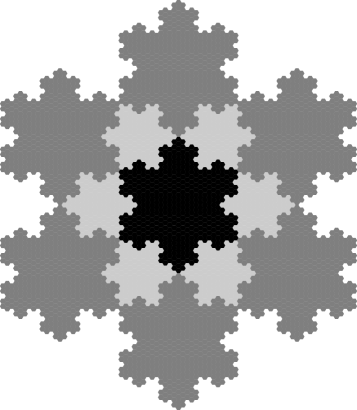
(a) $\mathcal{W}_{\eta,j}$ for a lattice originating from $\tau$ with $\tau^{2}-3\tau+3=0$, $w=2$ and $j=7$

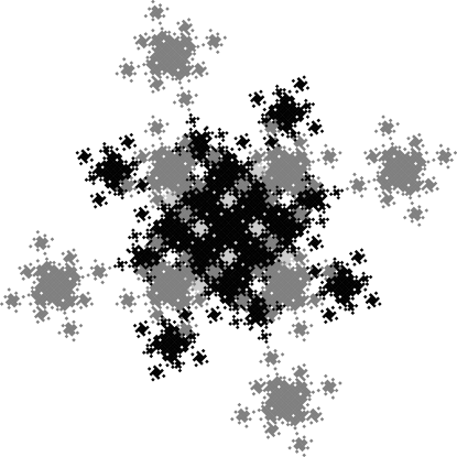
(b) $\mathcal{W}_{\eta,j}$ for a lattice coming from $\tau$ with $\tau^{2}-2\tau+2=0$, $w=4$ and $j=11$

Figure 9.1. Fundamental domains and characteristic sets $\mathcal{W}_{\eta}$. Each figure shows a fundamental domain. The light-gray coloured parts represent the approximations $\mathcal{W}_{\eta,j}$ of the characteristic sets $\mathcal{W}_{\eta}$.

Note that sometimes the set $W_{\eta}$ will also be called characteristic set for $\eta$, and analogously for the set $W_{\eta,j}$. In Figure 9.1 some of these characteristic sets, more precisely some approximations of the characteristic sets, are shown.

The following proposition deals with some properties of those defined sets.

Proposition 9.2 (Properties of the Characteristic Sets).

Let $\eta\in\mathcal{D}^{\bullet}$.

1. We have

   $$\mathcal{W}_{\eta}=\eta\tau^{-w}+\Phi^{-2w+1}\mathcal{F}.$$

2. The set $\mathcal{W}_{\eta}$ is compact.

3. We get

   $$\mathcal{W}_{\eta}=\overline{\bigcup_{j\in\mathbbm{N}_{0}}\mathcal{W}_{\eta,j}}=\overline{\lim_{j\to\infty}\mathcal{W}_{\eta,j}}.$$

4. The set $\left\lfloor{\mathcal{W}_{\eta,j}}\right\rceil_{{{T}},{j+w}}$ is indeed an approximation of $\mathcal{W}_{\eta}$, i.e., we have

   $$\mathcal{W}_{\eta}=\overline{\liminf_{j\in\mathbbm{N}_{0}}\left\lfloor{\mathcal{W}_{\eta,j}}\right\rceil_{{{T}},{j+w}}}=\overline{\limsup_{j\in\mathbbm{N}_{0}}\left\lfloor{\mathcal{W}_{\eta,j}}\right\rceil_{{{T}},{j+w}}}.$$

5. We have $\mathop{{\operatorname{int}}\thinspace\negthinspace}{\mathcal{W}_{\eta}}\subseteq\liminf_{j\in\mathbbm{N}_{0}}\left\lfloor{\mathcal{W}_{\eta,j}}\right\rceil_{{{T}},{j+w}}$.

6. We get $\mathcal{W}_{\eta}-\Phi^{-w}\eta\subseteq T$, and for $j\in\mathbbm{N}_{0}$ we obtain $\left\lfloor{\mathcal{W}_{\eta,j}}\right\rceil_{{{T}},{j+w}}-\Phi^{-w}\eta\subseteq T$.

7. For the Lebesgue measure of the characteristic set we obtain $\mathop{{\lambda}\thinspace\negthinspace}\mathchoice{\negthinspace}{\negthinspace}{}{}\left({\mathcal{W}_{\eta}}\right)=\mathop{{\lambda}\thinspace\negthinspace}\mathchoice{\negthinspace}{\negthinspace}{}{}\left({W_{\eta}}\right)$ and for its approximation $\mathop{{\lambda}\thinspace\negthinspace}\mathchoice{\negthinspace}{\negthinspace}{}{}\left({\left\lfloor{\mathcal{W}_{\eta,j}}\right\rceil_{{{T}},{j+w}}}\right)=\mathop{{\lambda}\thinspace\negthinspace}\mathchoice{\negthinspace}{\negthinspace}{}{}\left({W_{\eta,j}}\right)$.

8. Let $j\in\mathbbm{N}_{0}$, then

   $$\mathop{{\lambda}\thinspace\negthinspace}\mathchoice{\negthinspace}{\negthinspace}{}{}\left({\left\lfloor{\mathcal{W}_{\eta,j}}\right\rceil_{{{T}},{j+w}}}\right)=d_{\Lambda}E+\mathop{{\mathcal{O}}\thinspace\negthinspace}\mathchoice{\negthinspace}{\negthinspace}{}{}\left({\mu^{j}}\right)$$

   with $E$ and $\mu<1$ from Theorem 4.7.

9. The Lebesgue measure of $W_{\eta}$ is

   $$\mathop{{\lambda}\thinspace\negthinspace}\mathchoice{\negthinspace}{\negthinspace}{}{}\left({W_{\eta}}\right)=d_{\Lambda}E,$$

   again with $E$ from Theorem 4.7.

10. Let $j\in\mathbbm{N}_{0}$. We get

    $$\beta_{\eta,j}=\int_{x\in T}\mathop{{\left(\mathbbm{1}_{W_{\eta,j}}-\mathbbm{1}_{W_{\eta}}\right)}\thinspace\negthinspace}\mathchoice{\negthinspace}{\negthinspace}{}{}\left({x}\right)\operatorname{d}\negthinspace{}x=\mathop{{\mathcal{O}}\thinspace\negthinspace}\mathchoice{\negthinspace}{\negthinspace}{}{}\left({\mu^{j}}\right).$$

    Again $\mu<1$ can be found in Theorem 4.7.

Proof.

The proof is a straightforward generalisation of the proof in [13]. ∎

We can also determine the Lebesgue measure of the fundamental domain $\mathcal{F}$ defined in Section 7.

Remark 9.3 (Lebesgue Measure of the Fundamental Domain).

We get

$$\mathop{{\lambda}\thinspace\negthinspace}\mathchoice{\negthinspace}{\negthinspace}{}{}\left({\mathcal{F}}\right)=\rho^{n(2w-1)}Ed_{\Lambda}=\frac{\rho^{nw}d_{\Lambda}}{(\rho^{n}-1)w+1},$$

using (a) and (i) from Proposition 9.2 and $E$ from Theorem 4.7.

The next lemma makes the connection between the $w$-NAFs of elements of the lattice $\Lambda$ and the characteristic sets $W_{\eta,j}$.

Lemma 9.4.

Let $\eta\in\mathcal{D}^{\bullet}$, $j\geq 0$. Let $z\in\Lambda$ and let $\bm{\xi}\in\mathbf{NAF}_{w}^{{\mathsf{fin}}\bm{.}{0}}$ be its $w$-NAF. Then the following statements are equivalent:

1. The $j$th digit of $\bm{\xi}$ equals $\eta$.

2. The condition $\left\{{\Phi^{-(j+w)}z}\right\}_{\Lambda}\in W_{\eta,j}$ holds.

3. The inclusion $\left\{{\Phi^{-(j+w)}T_{z}}\right\}_{\Lambda}\subseteq W_{\eta,j}$ holds.

Proof.

The proof is a straightforward generalisation of the proof of the quadratic case in [13]. ∎

10. Counting the Occurrences of a non-zero Digit in a Region

In this section we will prove our main result on the asymptototic number of occurrences of a digit in a given region.

Note that Iverson’s notation $\left[{\mathit{expr}}\right]=1$ if $\mathit{expr}$ is true and $\left[{\mathit{expr}}\right]=0$ otherwise, cf. Graham, Knuth and Patashnik [11], will be used.

Theorem 10.1 (Counting Theorem).

Let $0\neq\eta\in\mathcal{D}$ and $N\in\mathbbm{R}$ with $N>0$. Further let $U\subseteq\mathbbm{R}^{n}$ be measurable with respect to the Lebesgue measure and bounded with $U\subseteq\mathop{{\mathcal{B}}\thinspace\negthinspace}\mathchoice{\negthinspace}{\negthinspace}{}{}\left({{0},{d}}\right)$ for a finite $d$, and set $\delta$ such that $\mathop{{\#}\thinspace\negthinspace}\mathchoice{\negthinspace}{\negthinspace}{}{}\left({\mathop{{\partial}\thinspace\negthinspace}\mathchoice{\negthinspace}{\negthinspace}{}{}\left({NU}\right)_{{{T}}}}\right)_{{{T}}}=\mathop{{\mathcal{O}}\thinspace\negthinspace}\mathchoice{\negthinspace}{\negthinspace}{}{}\left({N^{\delta}}\right)$ with $1\leq\delta<n$. We denote the number of occurrences of the digit $\eta$ in all integer width-$w$ non-adjacent forms with value in the region $NU$ by

$$\mathop{{Z_{\eta}}\thinspace\negthinspace}\mathchoice{\negthinspace}{\negthinspace}{}{}\left({N}\right)=\sum_{z\in NU\cap\Lambda}\sum_{j\in\mathbbm{N}_{0}}\left[{\text{$j$th digit of $z$ in its $w$-NAF{}-expansion equals $\eta$}}\right].$$

Then we get

$$\mathop{{Z_{\eta}}\thinspace\negthinspace}\mathchoice{\negthinspace}{\negthinspace}{}{}\left({N}\right)=N^{n}\mathop{{\lambda}\thinspace\negthinspace}\mathchoice{\negthinspace}{\negthinspace}{}{}\left({U}\right)E\log_{\rho}N+N^{n}\mathop{{\psi_{\eta}}\thinspace\negthinspace}\mathchoice{\negthinspace}{\negthinspace}{}{}\left({\log_{\rho}N}\right)+\mathop{{\mathcal{O}}\thinspace\negthinspace}\mathchoice{\negthinspace}{\negthinspace}{}{}\left({N^{\alpha}\log_{\rho}N}\right)+\mathop{{\mathcal{O}}\thinspace\negthinspace}\mathchoice{\negthinspace}{\negthinspace}{}{}\left({N^{\delta}\log_{\rho}N}\right),$$

in which the expressions described below are used. The Lebesgue measure on $\mathbbm{R}^{n}$ is denoted by $\lambda$. We have the constant of the expectation

$$E=\frac{1}{\rho^{n(w-1)}((\rho^{n}-1)w+1)},$$

cf. Theorem 4.7. Then there is the function

$$\mathop{{\psi_{\eta}}\thinspace\negthinspace}\mathchoice{\negthinspace}{\negthinspace}{}{}\left({x}\right)=\mathop{{\psi_{\eta,\mathcal{M}}}\thinspace\negthinspace}\mathchoice{\negthinspace}{\negthinspace}{}{}\left({x}\right)+\mathop{{\psi_{\eta,\mathcal{P}}}\thinspace\negthinspace}\mathchoice{\negthinspace}{\negthinspace}{}{}\left({x}\right)+\mathop{{\psi_{\eta,\mathcal{Q}}}\thinspace\negthinspace}\mathchoice{\negthinspace}{\negthinspace}{}{}\left({x}\right),$$

where

$$\mathop{{\psi_{\eta,\mathcal{M}}}\thinspace\negthinspace}\mathchoice{\negthinspace}{\negthinspace}{}{}\left({x}\right)=\mathop{{\lambda}\thinspace\negthinspace}\mathchoice{\negthinspace}{\negthinspace}{}{}\left({U}\right)\left(J_{0}+1-\left\{{x}\right\}\right)E,$$

$$\mathop{{\psi_{\eta,\mathcal{P}}}\thinspace\negthinspace}\mathchoice{\negthinspace}{\negthinspace}{}{}\left({x}\right)=\frac{\rho^{n(J_{0}-\left\{{x}\right\})}}{d_{\Lambda}}\sum_{j=0}^{\infty}\int_{y\in\left\{{\Phi^{-\left\lfloor{x}\right\rfloor-J_{0}}\rho^{x}U}\right\}_{{{T}},{j-w}}}\left(\mathop{{\mathbbm{1}_{W}}\thinspace\negthinspace}\mathchoice{\negthinspace}{\negthinspace}{}{}\left({\left\{{\Phi^{j-w}y}\right\}_{\Lambda}}\right)-\mathop{{\lambda}\thinspace\negthinspace}\mathchoice{\negthinspace}{\negthinspace}{}{}\left({W}\right)\right)\operatorname{d}\negthinspace{}y,$$

and

$$\psi_{\eta,\mathcal{Q}}=\frac{\mathop{{\lambda}\thinspace\negthinspace}\mathchoice{\negthinspace}{\negthinspace}{}{}\left({U}\right)}{d_{\Lambda}^{2}}\sum_{j=0}^{\infty}\beta_{j}.$$

We have $\alpha=n+\log_{\rho}\mu<n$, with $\mu=\left(1+\frac{1}{\rho^{n}w^{3}}\right)^{-1}<1$, and

$$J_{0}=\left\lfloor{\log_{\rho}d-\log_{\rho}B_{L}}\right\rfloor+1$$

with the constant $B_{L}$ of Proposition 5.2.

Further, let

$$\Phi=Q\mathop{{\operatorname{diag}}\thinspace\negthinspace}\mathchoice{\negthinspace}{\negthinspace}{}{}\left({\rho e^{i\theta_{1}},\dots,\rho e^{i\theta_{n}}}\right)Q^{-1},$$

where $Q$ is a regular matrix. If there is a $p\in\mathbbm{N}$ such that

$$Q\mathop{{\operatorname{diag}}\thinspace\negthinspace}\mathchoice{\negthinspace}{\negthinspace}{}{}\left({e^{i\theta_{1}p},\dots,e^{i\theta_{n}p}}\right)Q^{-1}U=U,$$

then $\psi_{\eta}$ is $p$-periodic. Moreover, if $\psi_{\eta}$ is $p$-periodic for some $p\in\mathbbm{N}$, then it is also continuous.

Remark 10.2.

Consider the main term of our result. When $N$ tends to infinity, we get the asymptotic formula

$$Z_{\eta}\sim N^{n}\mathop{{\lambda}\thinspace\negthinspace}\mathchoice{\negthinspace}{\negthinspace}{}{}\left({U}\right)E\log_{\rho}N.$$

This result is not surprising, since intuitively the number of lattice points in the region $NU$ corresponds to the Lebesgue measure $N^{n}\mathop{{\lambda}\thinspace\negthinspace}\mathchoice{\negthinspace}{\negthinspace}{}{}\left({U}\right)$ of this region, and each of those elements can be represented as an integer $w$-NAF with length about $\log_{\rho}N$. Therefore, using the expectation of Theorem 4.7, we get an explanation for this term.

Remark 10.3.

If $\delta=n$ in the theorem, then the statement stays true, but degenerates to

$$\mathop{{Z_{\eta}}\thinspace\negthinspace}\mathchoice{\negthinspace}{\negthinspace}{}{}\left({N}\right)=\mathop{{\mathcal{O}}\thinspace\negthinspace}\mathchoice{\negthinspace}{\negthinspace}{}{}\left({N^{n}\log_{\left\lvert{\tau}\right\rvert}N}\right).$$

This is a trivial result of Remark 10.2.

The proof of Theorem 10.1 follows the ideas used by Delange [6]. By Remark 10.3 we restrict ourselves to the case $\delta<n$.

We will use the following abbreviations. We omit the index $\eta$, i.e., we set $\mathop{{Z}\thinspace\negthinspace}\mathchoice{\negthinspace}{\negthinspace}{}{}\left({N}\right)\mathrel{\mathchoice{\vbox{\hbox{$\displaystyle:$}}}{\vbox{\hbox{$\textstyle:$}}}{\vbox{\hbox{$\scriptstyle:$}}}{\vbox{\hbox{$\scriptscriptstyle:$}}}{=}}\mathop{{Z_{\eta}}\thinspace\negthinspace}\mathchoice{\negthinspace}{\negthinspace}{}{}\left({N}\right)$, $W\mathrel{\mathchoice{\vbox{\hbox{$\displaystyle:$}}}{\vbox{\hbox{$\textstyle:$}}}{\vbox{\hbox{$\scriptstyle:$}}}{\vbox{\hbox{$\scriptscriptstyle:$}}}{=}}W_{\eta}$ and $W_{j}\mathrel{\mathchoice{\vbox{\hbox{$\displaystyle:$}}}{\vbox{\hbox{$\textstyle:$}}}{\vbox{\hbox{$\scriptstyle:$}}}{\vbox{\hbox{$\scriptscriptstyle:$}}}{=}}W_{\eta,j}$, and further we set $\beta_{j}\mathrel{\mathchoice{\vbox{\hbox{$\displaystyle:$}}}{\vbox{\hbox{$\textstyle:$}}}{\vbox{\hbox{$\scriptstyle:$}}}{\vbox{\hbox{$\scriptscriptstyle:$}}}{=}}\beta_{\eta,j}$, cf. Proposition 9.2. By $\log$ we will denote the logarithm to the base $\rho$, i.e., $\log x=\log_{\rho}x$. These abbreviations will be used throughout the remaining section.

Proof of Theorem 10.1.

By assumption every element of $\Lambda$ is represented by a unique element of $\mathbf{NAF}_{w}^{{\mathsf{fin}}\bm{.}{0}}$. To count the occurrences of the digit $\eta$ in $NU$, we sum up $1$ over all lattice points $z\in NU\cap\Lambda$ and for each $z$ over all digits in the corresponding $w$-NAF equal to $\eta$. Thus we get

$$\mathop{{Z}\thinspace\negthinspace}\mathchoice{\negthinspace}{\negthinspace}{}{}\left({N}\right)=\sum_{z\in NU\cap\Lambda}\sum_{j\in\mathbbm{N}_{0}}\left[{\text{$j$th digit of $w$-NAF{} of $z$ equals $\eta$}}\right].$$

The inner sum over $j\in\mathbbm{N}_{0}$ is finite, we will choose a large enough upper bound $J$ later in Lemma 10.4.

Using

$$\left[{\text{$j$th digit of $w$-NAF{} of $z$ equals $\eta$}}\right]=\mathop{{\mathbbm{1}_{W_{j}}}\thinspace\negthinspace}\mathchoice{\negthinspace}{\negthinspace}{}{}\left({\left\{{\Phi^{-j-w}z}\right\}_{\Lambda}}\right)$$

from Lemma 9.4 yields

$$\mathop{{Z}\thinspace\negthinspace}\mathchoice{\negthinspace}{\negthinspace}{}{}\left({N}\right)=\sum_{j=0}^{J}\sum_{z\in NU\cap\Lambda}\mathop{{\mathbbm{1}_{W_{j}}}\thinspace\negthinspace}\mathchoice{\negthinspace}{\negthinspace}{}{}\left({\left\{{\Phi^{-j-w}z}\right\}_{\Lambda}}\right),$$

where additionally the order of summation was changed. This enables us to rewrite the sum over $z$ as an integral

$$\begin{split}\mathop{{Z}\thinspace\negthinspace}\mathchoice{\negthinspace}{\negthinspace}{}{}\left({N}\right)&=\sum_{j=0}^{J}\sum_{z\in NU\cap\Lambda}\frac{1}{\mathop{{\lambda}\thinspace\negthinspace}\mathchoice{\negthinspace}{\negthinspace}{}{}\left({T_{z}}\right)}\int_{x\in T_{z}}\mathop{{\mathbbm{1}_{W_{j}}}\thinspace\negthinspace}\mathchoice{\negthinspace}{\negthinspace}{}{}\left({\left\{{\Phi^{-j-w}x}\right\}_{\Lambda}}\right)\operatorname{d}\negthinspace{}x\\ &=\frac{1}{\mathop{{\lambda}\thinspace\negthinspace}\mathchoice{\negthinspace}{\negthinspace}{}{}\left({T}\right)}\sum_{j=0}^{J}\int_{x\in\left\lfloor{NU}\right\rceil_{{{T}}}}\mathop{{\mathbbm{1}_{W_{j}}}\thinspace\negthinspace}\mathchoice{\negthinspace}{\negthinspace}{}{}\left({\left\{{\Phi^{-j-w}x}\right\}_{\Lambda}}\right)\operatorname{d}\negthinspace{}x.\end{split}$$

We split up the integrals into the ones over $NU$ and others over the remaining region and get

$$\mathop{{Z}\thinspace\negthinspace}\mathchoice{\negthinspace}{\negthinspace}{}{}\left({N}\right)=\frac{1}{\mathop{{\lambda}\thinspace\negthinspace}\mathchoice{\negthinspace}{\negthinspace}{}{}\left({T}\right)}\sum_{j=0}^{J}\int_{x\in NU}\mathop{{\mathbbm{1}_{W_{j}}}\thinspace\negthinspace}\mathchoice{\negthinspace}{\negthinspace}{}{}\left({\left\{{\Phi^{-j-w}x}\right\}_{\Lambda}}\right)\operatorname{d}\negthinspace{}x+\mathop{{\mathcal{F}_{\eta}}\thinspace\negthinspace}\mathchoice{\negthinspace}{\negthinspace}{}{}\left({N}\right),$$

in which $\mathop{{\mathcal{F}_{\eta}}\thinspace\negthinspace}\mathchoice{\negthinspace}{\negthinspace}{}{}\left({N}\right)$ contains all integrals (with appropriate signs) over regions $\left\lfloor{NU}\right\rceil_{{{T}}}\setminus NU$ and $NU\setminus\left\lfloor{NU}\right\rceil_{{{T}}}$.

By substituting $x=\Phi^{J}y$, $\operatorname{d}\negthinspace{}x=\left\lvert{\det\Phi}\right\rvert^{J}\operatorname{d}\negthinspace{}y=\rho^{nJ}\operatorname{d}\negthinspace{}y$ we obtain

$$\mathop{{Z}\thinspace\negthinspace}\mathchoice{\negthinspace}{\negthinspace}{}{}\left({N}\right)=\frac{\rho^{nJ}}{\mathop{{\lambda}\thinspace\negthinspace}\mathchoice{\negthinspace}{\negthinspace}{}{}\left({T}\right)}\sum_{j=0}^{J}\int_{y\in\Phi^{-J}NU}\mathop{{\mathbbm{1}_{W_{j}}}\thinspace\negthinspace}\mathchoice{\negthinspace}{\negthinspace}{}{}\left({\left\{{\Phi^{J-j-w}y}\right\}_{\Lambda}}\right)\operatorname{d}\negthinspace{}y+\mathop{{\mathcal{F}_{\eta}}\thinspace\negthinspace}\mathchoice{\negthinspace}{\negthinspace}{}{}\left({N}\right).$$

Reversing the order of summation yields

$$\mathop{{Z}\thinspace\negthinspace}\mathchoice{\negthinspace}{\negthinspace}{}{}\left({N}\right)=\frac{\rho^{nJ}}{\mathop{{\lambda}\thinspace\negthinspace}\mathchoice{\negthinspace}{\negthinspace}{}{}\left({T}\right)}\sum_{j=0}^{J}\int_{y\in\Phi^{-J}NU}\mathop{{\mathbbm{1}_{W_{J-j}}}\thinspace\negthinspace}\mathchoice{\negthinspace}{\negthinspace}{}{}\left({\left\{{\Phi^{j-w}y}\right\}_{\Lambda}}\right)\operatorname{d}\negthinspace{}y+\mathop{{\mathcal{F}_{\eta}}\thinspace\negthinspace}\mathchoice{\negthinspace}{\negthinspace}{}{}\left({N}\right).$$

We rewrite this as

$$\begin{split}\mathop{{Z}\thinspace\negthinspace}\mathchoice{\negthinspace}{\negthinspace}{}{}\left({N}\right)&=\frac{\rho^{nJ}}{\mathop{{\lambda}\thinspace\negthinspace}\mathchoice{\negthinspace}{\negthinspace}{}{}\left({T}\right)}(J+1)\mathop{{\lambda}\thinspace\negthinspace}\mathchoice{\negthinspace}{\negthinspace}{}{}\left({W}\right)\int_{y\in\Phi^{-J}NU}\operatorname{d}\negthinspace{}y\\ &\phantom{=}+\frac{\rho^{nJ}}{\mathop{{\lambda}\thinspace\negthinspace}\mathchoice{\negthinspace}{\negthinspace}{}{}\left({T}\right)}\sum_{j=0}^{J}\int_{y\in\Phi^{-J}NU}\left(\mathop{{\mathbbm{1}_{W}}\thinspace\negthinspace}\mathchoice{\negthinspace}{\negthinspace}{}{}\left({\left\{{\Phi^{j-w}y}\right\}_{\Lambda}}\right)-\mathop{{\lambda}\thinspace\negthinspace}\mathchoice{\negthinspace}{\negthinspace}{}{}\left({W}\right)\right)\operatorname{d}\negthinspace{}y\\ &\phantom{=}+\frac{\rho^{nJ}}{\mathop{{\lambda}\thinspace\negthinspace}\mathchoice{\negthinspace}{\negthinspace}{}{}\left({T}\right)}\sum_{j=0}^{J}\int_{y\in\Phi^{-J}NU}\left(\mathop{{\mathbbm{1}_{W_{J-j}}}\thinspace\negthinspace}\mathchoice{\negthinspace}{\negthinspace}{}{}\left({\left\{{\Phi^{j-w}y}\right\}_{\Lambda}}\right)-\mathop{{\mathbbm{1}_{W}}\thinspace\negthinspace}\mathchoice{\negthinspace}{\negthinspace}{}{}\left({\left\{{\Phi^{j-w}y}\right\}_{\Lambda}}\right)\right)\operatorname{d}\negthinspace{}y\\ &\phantom{=}+\mathop{{\mathcal{F}_{\eta}}\thinspace\negthinspace}\mathchoice{\negthinspace}{\negthinspace}{}{}\left({N}\right).\end{split}$$

With $\Phi^{-J}NU=\left\lfloor{\Phi^{-J}NU}\right\rfloor_{{{T}},{j-w}}\cup\left\{{\Phi^{-J}NU}\right\}_{{{T}},{j-w}}$ for each area of integration we get

$$\mathop{{Z}\thinspace\negthinspace}\mathchoice{\negthinspace}{\negthinspace}{}{}\left({N}\right)=\mathop{{\mathcal{M}_{\eta}}\thinspace\negthinspace}\mathchoice{\negthinspace}{\negthinspace}{}{}\left({N}\right)+\mathop{{\mathcal{Z}_{\eta}}\thinspace\negthinspace}\mathchoice{\negthinspace}{\negthinspace}{}{}\left({N}\right)+\mathop{{\mathcal{P}_{\eta}}\thinspace\negthinspace}\mathchoice{\negthinspace}{\negthinspace}{}{}\left({N}\right)+\mathop{{\mathcal{Q}_{\eta}}\thinspace\negthinspace}\mathchoice{\negthinspace}{\negthinspace}{}{}\left({N}\right)+\mathop{{\mathcal{S}_{\eta}}\thinspace\negthinspace}\mathchoice{\negthinspace}{\negthinspace}{}{}\left({N}\right)+\mathop{{\mathcal{F}_{\eta}}\thinspace\negthinspace}\mathchoice{\negthinspace}{\negthinspace}{}{}\left({N}\right),$$

in which $\mathcal{M}_{\eta}$ is “The Main Part”, see Lemma 10.6,

$$\mathop{{\mathcal{M}_{\eta}}\thinspace\negthinspace}\mathchoice{\negthinspace}{\negthinspace}{}{}\left({N}\right)=\frac{\rho^{nJ}}{\mathop{{\lambda}\thinspace\negthinspace}\mathchoice{\negthinspace}{\negthinspace}{}{}\left({T}\right)}(J+1)\mathop{{\lambda}\thinspace\negthinspace}\mathchoice{\negthinspace}{\negthinspace}{}{}\left({W}\right)\int_{y\in\Phi^{-J}NU}\operatorname{d}\negthinspace{}y,$$ (10.1a)

$$\mathcal{Z}_{\eta}$$ is “The Zero Part”, see Lemma 10.7,

$$\mathop{{\mathcal{Z}_{\eta}}\thinspace\negthinspace}\mathchoice{\negthinspace}{\negthinspace}{}{}\left({N}\right)=\frac{\rho^{nJ}}{\mathop{{\lambda}\thinspace\negthinspace}\mathchoice{\negthinspace}{\negthinspace}{}{}\left({T}\right)}\sum_{j=0}^{J}\int_{y\in\left\lfloor{\Phi^{-J}NU}\right\rfloor_{{{T}},{j-w}}}\left(\mathop{{\mathbbm{1}_{W}}\thinspace\negthinspace}\mathchoice{\negthinspace}{\negthinspace}{}{}\left({\left\{{\Phi^{j-w}y}\right\}_{\Lambda}}\right)-\mathop{{\lambda}\thinspace\negthinspace}\mathchoice{\negthinspace}{\negthinspace}{}{}\left({W}\right)\right)\operatorname{d}\negthinspace{}y,$$ (10.1b)

$$\mathcal{P}_{\eta}$$ is “The Periodic Part”, see Lemma 10.8,

$$\mathop{{\mathcal{P}_{\eta}}\thinspace\negthinspace}\mathchoice{\negthinspace}{\negthinspace}{}{}\left({N}\right)=\frac{\rho^{nJ}}{\mathop{{\lambda}\thinspace\negthinspace}\mathchoice{\negthinspace}{\negthinspace}{}{}\left({T}\right)}\sum_{j=0}^{J}\int_{y\in\left\{{\Phi^{-J}NU}\right\}_{{{T}},{j-w}}}\left(\mathop{{\mathbbm{1}_{W}}\thinspace\negthinspace}\mathchoice{\negthinspace}{\negthinspace}{}{}\left({\left\{{\Phi^{j-w}y}\right\}_{\Lambda}}\right)-\mathop{{\lambda}\thinspace\negthinspace}\mathchoice{\negthinspace}{\negthinspace}{}{}\left({W}\right)\right)\operatorname{d}\negthinspace{}y,$$ (10.1c)

$$\mathcal{Q}_{\eta}$$ is “The Other Part”, see Lemma 10.9,

$$\mathop{{\mathcal{Q}_{\eta}}\thinspace\negthinspace}\mathchoice{\negthinspace}{\negthinspace}{}{}\left({N}\right)=\frac{\rho^{nJ}}{\mathop{{\lambda}\thinspace\negthinspace}\mathchoice{\negthinspace}{\negthinspace}{}{}\left({T}\right)}\sum_{j=0}^{J}\int_{y\in\left\lfloor{\Phi^{-J}NU}\right\rfloor_{{{T}},{j-w}}}\mathop{{\left(\mathbbm{1}_{W_{J-j}}-\mathbbm{1}_{W}\right)}\thinspace\negthinspace}\mathchoice{\negthinspace}{\negthinspace}{}{}\left({\left\{{\Phi^{j-w}y}\right\}_{\Lambda}}\right)\operatorname{d}\negthinspace{}y,$$ (10.1d)

$$\mathcal{S}_{\eta}$$ is “The Small Part”, see Lemma 10.10,

$$\mathop{{\mathcal{S}_{\eta}}\thinspace\negthinspace}\mathchoice{\negthinspace}{\negthinspace}{}{}\left({N}\right)=\frac{\rho^{nJ}}{\mathop{{\lambda}\thinspace\negthinspace}\mathchoice{\negthinspace}{\negthinspace}{}{}\left({T}\right)}\sum_{j=0}^{J}\int_{y\in\left\{{\Phi^{-J}NU}\right\}_{{{T}},{j-w}}}\mathop{{\left(\mathbbm{1}_{W_{J-j}}-\mathbbm{1}_{W}\right)}\thinspace\negthinspace}\mathchoice{\negthinspace}{\negthinspace}{}{}\left({\left\{{\Phi^{j-w}y}\right\}_{\Lambda}}\right)\operatorname{d}\negthinspace{}y$$ (10.1e)

and $$\mathcal{F}_{\eta}$$ is “The Fractional Cells Part”, see Lemma 10.11,

$$\begin{split}\mathop{{\mathcal{F}_{\eta}}\thinspace\negthinspace}\mathchoice{\negthinspace}{\negthinspace}{}{}\left({N}\right)&=\frac{1}{\mathop{{\lambda}\thinspace\negthinspace}\mathchoice{\negthinspace}{\negthinspace}{}{}\left({T}\right)}\sum_{j=0}^{J}\int_{x\in\left\lfloor{NU}\right\rceil_{{{T}}}\setminus NU}\mathop{{\mathbbm{1}_{W_{j}}}\thinspace\negthinspace}\mathchoice{\negthinspace}{\negthinspace}{}{}\left({\left\{{\Phi^{-j-w}x}\right\}_{\Lambda}}\right)\operatorname{d}\negthinspace{}x\\ &\phantom{=}-\frac{1}{\mathop{{\lambda}\thinspace\negthinspace}\mathchoice{\negthinspace}{\negthinspace}{}{}\left({T}\right)}\sum_{j=0}^{J}\int_{x\in NU\setminus\left\lfloor{NU}\right\rceil_{{{T}}}}\mathop{{\mathbbm{1}_{W_{j}}}\thinspace\negthinspace}\mathchoice{\negthinspace}{\negthinspace}{}{}\left({\left\{{\Phi^{-j-w}x}\right\}_{\Lambda}}\right)\operatorname{d}\negthinspace{}x.\end{split}$$ (10.1f)

To complete the proof we have to deal with the choice of $J$, see Lemma 10.4, as well as with each of the parts in (10.1), see Lemmata 10.6 to 10.11. The continuity of $\psi_{\eta}$ is checked in Lemma 10.12. ∎

Lemma 10.4 (Choosing $J$).

Let $N\in\mathbbm{R}_{\geq 0}$. Then every $w$-NAF of $\mathbf{NAF}_{w}^{{\mathsf{fin}}\bm{.}{0}}$ with value in $NU$ has at most $J+1$ digits, where

$$J=\left\lfloor{\log N}\right\rfloor+J_{0}$$

with

$$J_{0}=\left\lfloor{\log d-\log B_{L}}\right\rfloor+1$$

with $B_{L}$ of Proposition 5.2.

Proof.

Let $z\in NU$, $z\neq 0$, with its corresponding $w$-NAF $\bm{\xi}\in\mathbf{NAF}_{w}^{{\mathsf{fin}}\bm{.}{0}}$, and let $j\in\mathbbm{N}_{0}$ be the largest index such that the digit $\xi_{j}$ is non-zero. By using Corollary 5.3, we conclude that

$$\rho^{j}B_{L}\leq\left\lVert{z}\right\rVert<Nd.$$

This means

$$j<\log N+\log d-\log B_{L},$$

and thus we have

$$j\leq\left\lfloor{\log N+\log d-\log B_{L}}\right\rfloor\leq\left\lfloor{\log N}\right\rfloor+\left\lfloor{\log d-\log B_{L}}\right\rfloor+1.$$

Defining the right hand side of this inequality as $J$ finishes the proof. ∎

Remark 10.5.

For the parameter used in the region of integration in the proof of Theorem 10.1 we get

$$\left\lvert{\det\left(\Phi^{-J}N\right)}\right\rvert=\mathop{{\mathcal{O}}\thinspace\negthinspace}\mathchoice{\negthinspace}{\negthinspace}{}{}\left({1}\right).$$

In particular, we get $\left\lVert{\Phi^{-J}N}\right\rVert=\mathop{{\mathcal{O}}\thinspace\negthinspace}\mathchoice{\negthinspace}{\negthinspace}{}{}\left({1}\right)$.

Proof.

We have

$$\left\lvert{\det\left(\Phi^{-J}N\right)}\right\rvert=\left(\rho^{-J}N\right)^{n}.$$

With $J$ of Lemma 10.4 we obtain

$$\rho^{-J}N=\rho^{-\left\lfloor{\log N}\right\rfloor-J_{0}}\rho^{\log N}=\rho^{\log N-\left\lfloor{\log N}\right\rfloor-J_{0}}=\rho^{\left\{{\log N}\right\}-J_{0}}.$$

Since $\rho^{\left\{{\log N}\right\}-J_{0}}$ is bounded by $\rho^{1-J_{0}}$, it is $\mathop{{\mathcal{O}}\thinspace\negthinspace}\mathchoice{\negthinspace}{\negthinspace}{}{}\left({1}\right)$. Therefore $\det\left(\Phi^{-J}N\right)$ is $\mathop{{\mathcal{O}}\thinspace\negthinspace}\mathchoice{\negthinspace}{\negthinspace}{}{}\left({1}\right)$. Since $\left\lVert{\Phi^{-1}}\right\rVert=\rho^{-1}$ we conclude that $\left\lVert{\Phi^{-J}N}\right\rVert$ is $\mathop{{\mathcal{O}}\thinspace\negthinspace}\mathchoice{\negthinspace}{\negthinspace}{}{}\left({1}\right)$. ∎

Lemma 10.6 (The Main Part).

For (10.1a) in the proof of Theorem 10.1 we get

$$\mathop{{\mathcal{M}_{\eta}}\thinspace\negthinspace}\mathchoice{\negthinspace}{\negthinspace}{}{}\left({N}\right)=N^{n}\mathop{{\lambda}\thinspace\negthinspace}\mathchoice{\negthinspace}{\negthinspace}{}{}\left({U}\right)E\log N+N^{n}\mathop{{\psi_{\eta,\mathcal{M}}}\thinspace\negthinspace}\mathchoice{\negthinspace}{\negthinspace}{}{}\left({\log N}\right)$$

with a $1$-periodic function $\psi_{\eta,\mathcal{M}}$,

$$\mathop{{\psi_{\eta,\mathcal{M}}}\thinspace\negthinspace}\mathchoice{\negthinspace}{\negthinspace}{}{}\left({x}\right)=\mathop{{\lambda}\thinspace\negthinspace}\mathchoice{\negthinspace}{\negthinspace}{}{}\left({U}\right)\left(J_{0}+1-\left\{{x}\right\}\right)E$$

and $E$ of Theorem 4.7.

Proof.

We have

$$\mathop{{\mathcal{M}_{\eta}}\thinspace\negthinspace}\mathchoice{\negthinspace}{\negthinspace}{}{}\left({N}\right)=\frac{\rho^{nJ}}{\mathop{{\lambda}\thinspace\negthinspace}\mathchoice{\negthinspace}{\negthinspace}{}{}\left({T}\right)}(J+1)\mathop{{\lambda}\thinspace\negthinspace}\mathchoice{\negthinspace}{\negthinspace}{}{}\left({W}\right)\int_{y\in\Phi^{-J}NU}\operatorname{d}\negthinspace{}y.$$

As $\mathop{{\lambda}\thinspace\negthinspace}\mathchoice{\negthinspace}{\negthinspace}{}{}\left({\Phi^{-J}NU}\right)=\rho^{-nJ}N^{n}\mathop{{\lambda}\thinspace\negthinspace}\mathchoice{\negthinspace}{\negthinspace}{}{}\left({U}\right)$ we obtain

$$\mathop{{\mathcal{M}_{\eta}}\thinspace\negthinspace}\mathchoice{\negthinspace}{\negthinspace}{}{}\left({N}\right)=\frac{\mathop{{\lambda}\thinspace\negthinspace}\mathchoice{\negthinspace}{\negthinspace}{}{}\left({W}\right)}{\mathop{{\lambda}\thinspace\negthinspace}\mathchoice{\negthinspace}{\negthinspace}{}{}\left({T}\right)}(J+1)N^{n}\mathop{{\lambda}\thinspace\negthinspace}\mathchoice{\negthinspace}{\negthinspace}{}{}\left({U}\right).$$

By taking $\mathop{{\lambda}\thinspace\negthinspace}\mathchoice{\negthinspace}{\negthinspace}{}{}\left({W}\right)=\mathop{{\lambda}\thinspace\negthinspace}\mathchoice{\negthinspace}{\negthinspace}{}{}\left({T}\right)E$ from (i) of Proposition 9.2 and $J$ from Lemma 10.4 we get

$$\mathop{{\mathcal{M}_{\eta}}\thinspace\negthinspace}\mathchoice{\negthinspace}{\negthinspace}{}{}\left({N}\right)=N^{n}\mathop{{\lambda}\thinspace\negthinspace}\mathchoice{\negthinspace}{\negthinspace}{}{}\left({U}\right)E\left(\left\lfloor{\log N}\right\rfloor+J_{0}+1\right).$$

Finally, the desired result follows by using $\left\lfloor{x}\right\rfloor=x-\left\{{x}\right\}$. ∎

Lemma 10.7 (The Zero Part).

For (10.1b) in the proof of Theorem 10.1 we get

$$\mathop{{\mathcal{Z}_{\eta}}\thinspace\negthinspace}\mathchoice{\negthinspace}{\negthinspace}{}{}\left({N}\right)=0.$$

Proof.

Consider the integral

$$I_{j}\mathrel{\mathchoice{\vbox{\hbox{$\displaystyle:$}}}{\vbox{\hbox{$\textstyle:$}}}{\vbox{\hbox{$\scriptstyle:$}}}{\vbox{\hbox{$\scriptscriptstyle:$}}}{=}}\int_{y\in\left\lfloor{\Phi^{-J}NU}\right\rfloor_{{{T}},{j-w}}}\left(\mathop{{\mathbbm{1}_{W}}\thinspace\negthinspace}\mathchoice{\negthinspace}{\negthinspace}{}{}\left({\left\{{\Phi^{j-w}y}\right\}_{\Lambda}}\right)-\mathop{{\lambda}\thinspace\negthinspace}\mathchoice{\negthinspace}{\negthinspace}{}{}\left({W}\right)\right)\operatorname{d}\negthinspace{}y.$$

We can rewrite the region of integration as

$$\left\lfloor{\Phi^{-J}NU}\right\rfloor_{{{T}},{j-w}}=\Phi^{-(j-w)}\left\lfloor{\Phi^{j-w}\Phi^{-J}NU}\right\rfloor_{{{T}}}=\Phi^{-(j-w)}\bigcup_{z\in R_{j-w}}T_{z}$$

for some appropriate $R_{j-w}\subseteq\Lambda$. Substituting $x=\Phi^{j-w}y$, $\operatorname{d}\negthinspace{}x=\rho^{n(j-w)}\operatorname{d}\negthinspace{}y$ yields

$$I_{j}=\rho^{-n(j-w)}\int_{x\in\bigcup_{z\in R_{j-w}}T_{z}}\left(\mathop{{\mathbbm{1}_{W}}\thinspace\negthinspace}\mathchoice{\negthinspace}{\negthinspace}{}{}\left({\left\{{x}\right\}_{\Lambda}}\right)-\mathop{{\lambda}\thinspace\negthinspace}\mathchoice{\negthinspace}{\negthinspace}{}{}\left({W}\right)\right)\operatorname{d}\negthinspace{}x.$$

We split up the integral and eliminate the fractional part $\left\{{x}\right\}_{\Lambda}$ by translation to get

$$I_{j}=\rho^{-n(j-w)}\sum_{z\in R_{j-w}}\underbrace{\int_{x\in T}\left(\mathop{{\mathbbm{1}_{W}}\thinspace\negthinspace}\mathchoice{\negthinspace}{\negthinspace}{}{}\left({x}\right)-\mathop{{\lambda}\thinspace\negthinspace}\mathchoice{\negthinspace}{\negthinspace}{}{}\left({W}\right)\right)\operatorname{d}\negthinspace{}x}_{=0}.$$

Thus, for all $j\in\mathbbm{N}_{0}$ we obtain $I_{j}=0$, and therefore $\mathop{{\mathcal{Z}_{\eta}}\thinspace\negthinspace}\mathchoice{\negthinspace}{\negthinspace}{}{}\left({N}\right)=0$. ∎

Lemma 10.8 (The Periodic Part).

For (10.1c) in the proof of Theorem 10.1 we get

$$\mathop{{\mathcal{P}_{\eta}}\thinspace\negthinspace}\mathchoice{\negthinspace}{\negthinspace}{}{}\left({N}\right)=N^{n}\mathop{{\psi_{\eta,\mathcal{P}}}\thinspace\negthinspace}\mathchoice{\negthinspace}{\negthinspace}{}{}\left({\log N}\right)+\mathop{{\mathcal{O}}\thinspace\negthinspace}\mathchoice{\negthinspace}{\negthinspace}{}{}\left({N^{\delta}}\right)$$

with a function $\psi_{\eta,\mathcal{P}}$,

$$\mathop{{\psi_{\eta,\mathcal{P}}}\thinspace\negthinspace}\mathchoice{\negthinspace}{\negthinspace}{}{}\left({x}\right)=\frac{\rho^{n(J_{0}-\left\{{x}\right\})}}{\mathop{{\lambda}\thinspace\negthinspace}\mathchoice{\negthinspace}{\negthinspace}{}{}\left({T}\right)}\sum_{j=0}^{\infty}\int_{y\in\left\{{\Phi^{-\left\lfloor{x}\right\rfloor-J_{0}}\rho^{x}U}\right\}_{{{T}},{j-w}}}\left(\mathop{{\mathbbm{1}_{W}}\thinspace\negthinspace}\mathchoice{\negthinspace}{\negthinspace}{}{}\left({\left\{{\Phi^{j-w}y}\right\}_{\Lambda}}\right)-\mathop{{\lambda}\thinspace\negthinspace}\mathchoice{\negthinspace}{\negthinspace}{}{}\left({W}\right)\right)\operatorname{d}\negthinspace{}y.$$

Let

$$\Phi=Q\mathop{{\operatorname{diag}}\thinspace\negthinspace}\mathchoice{\negthinspace}{\negthinspace}{}{}\left({\rho e^{i\theta_{1}},\dots,\rho e^{i\theta_{n}}}\right)Q^{-1},$$

where $Q$ is a regular matrix. If there is a $p\in\mathbbm{N}$ such that

$$Q\mathop{{\operatorname{diag}}\thinspace\negthinspace}\mathchoice{\negthinspace}{\negthinspace}{}{}\left({e^{i\theta_{1}p},\dots,e^{i\theta_{n}p}}\right)Q^{-1}U=U,$$ (10.2)

then $\psi_{\eta,\mathcal{P}}$ is $p$-periodic.

Proof.

Consider

$$I_{j}\mathrel{\mathchoice{\vbox{\hbox{$\displaystyle:$}}}{\vbox{\hbox{$\textstyle:$}}}{\vbox{\hbox{$\scriptstyle:$}}}{\vbox{\hbox{$\scriptscriptstyle:$}}}{=}}\int_{y\in\left\{{\Phi^{-J}NU}\right\}_{{{T}},{j-w}}}\left(\mathop{{\mathbbm{1}_{W}}\thinspace\negthinspace}\mathchoice{\negthinspace}{\negthinspace}{}{}\left({\left\{{\Phi^{j-w}y}\right\}_{\Lambda}}\right)-\mathop{{\lambda}\thinspace\negthinspace}\mathchoice{\negthinspace}{\negthinspace}{}{}\left({W}\right)\right)\operatorname{d}\negthinspace{}y.$$

The region of integration satisfies

$$\begin{split}\left\{{\Phi^{-J}NU}\right\}_{{{T}},{j-w}}\subseteq\mathop{{\partial}\thinspace\negthinspace}\mathchoice{\negthinspace}{\negthinspace}{}{}\left({\Phi^{-J}NU}\right)_{{{T}},{j-w}}=\Phi^{-(j-w)}\bigcup_{z\in R_{j-w}}T_{z}\end{split}$$ (10.3)

for some appropriate $R_{j-w}\subseteq\Lambda$.

We use the triangle inequality and substitute $x=\Phi^{j-w}y$, $\operatorname{d}\negthinspace{}x=\rho^{n(j-w)}\operatorname{d}\negthinspace{}y$ in the integral to get

$$\left\lvert{I_{j}}\right\rvert\leq\rho^{-n(j-w)}\int_{x\in\bigcup_{z\in R_{j-w}}T_{z}}\underbrace{\left\lvert{\mathop{{\mathbbm{1}_{W}}\thinspace\negthinspace}\mathchoice{\negthinspace}{\negthinspace}{}{}\left({\left\{{x}\right\}_{\Lambda}}\right)-\mathop{{\lambda}\thinspace\negthinspace}\mathchoice{\negthinspace}{\negthinspace}{}{}\left({W}\right)}\right\rvert}_{\leq 1+\mathop{{\lambda}\thinspace\negthinspace}\mathchoice{\negthinspace}{\negthinspace}{}{}\left({W}\right)}\operatorname{d}\negthinspace{}x.$$

After splitting up the integral and using translation to eliminate the fractional part, we get

$$\left\lvert{I_{j}}\right\rvert\leq\rho^{-n(j-w)}\left(1+\mathop{{\lambda}\thinspace\negthinspace}\mathchoice{\negthinspace}{\negthinspace}{}{}\left({W}\right)\right)\sum_{z\in R_{j-w}}\int_{x\in T}\operatorname{d}\negthinspace{}x=\rho^{-n(j-w)}\left(1+\mathop{{\lambda}\thinspace\negthinspace}\mathchoice{\negthinspace}{\negthinspace}{}{}\left({W}\right)\right)\mathop{{\lambda}\thinspace\negthinspace}\mathchoice{\negthinspace}{\negthinspace}{}{}\left({T}\right)\mathop{{\#}\thinspace\negthinspace}\mathchoice{\negthinspace}{\negthinspace}{}{}\left({R_{j-w}}\right).$$

Using $\mathop{{\#}\thinspace\negthinspace}\mathchoice{\negthinspace}{\negthinspace}{}{}\left({\mathop{{\partial}\thinspace\negthinspace}\mathchoice{\negthinspace}{\negthinspace}{}{}\left({\Psi U}\right)_{{{T}}}}\right)_{{{T}}}=\mathop{{\mathcal{O}}\thinspace\negthinspace}\mathchoice{\negthinspace}{\negthinspace}{}{}\left({\left\lvert{\det\Psi}\right\rvert^{\delta/n}}\right)$ as assumed and (10.3) we gain

$$\mathop{{\#}\thinspace\negthinspace}\mathchoice{\negthinspace}{\negthinspace}{}{}\left({R_{j-w}}\right)=\left\lvert{\det\left(\Phi^{-J}N\Phi^{j-w}\right)}\right\rvert^{\delta/n}=\mathop{{\mathcal{O}}\thinspace\negthinspace}\mathchoice{\negthinspace}{\negthinspace}{}{}\left({\rho^{(j-w)\delta}}\right),$$

because $\left\lvert{\det\left(\Phi^{-J}N\right)}\right\rvert=\mathop{{\mathcal{O}}\thinspace\negthinspace}\mathchoice{\negthinspace}{\negthinspace}{}{}\left({1}\right)$, see Remark 10.5, and $\left\lvert{\det\Phi}\right\rvert=\rho^{n}$. Thus

$$\left\lvert{I_{j}}\right\rvert=\mathop{{\mathcal{O}}\thinspace\negthinspace}\mathchoice{\negthinspace}{\negthinspace}{}{}\left({\rho^{\delta(j-w)-n(j-w)}}\right)=\mathop{{\mathcal{O}}\thinspace\negthinspace}\mathchoice{\negthinspace}{\negthinspace}{}{}\left({\rho^{(\delta-n)j}}\right).$$

Now we want to make the summation in $\mathcal{P}_{\eta}$ independent from $J$, so we consider

$$I\mathrel{\mathchoice{\vbox{\hbox{$\displaystyle:$}}}{\vbox{\hbox{$\textstyle:$}}}{\vbox{\hbox{$\scriptstyle:$}}}{\vbox{\hbox{$\scriptscriptstyle:$}}}{=}}\frac{\rho^{nJ}}{\mathop{{\lambda}\thinspace\negthinspace}\mathchoice{\negthinspace}{\negthinspace}{}{}\left({T}\right)}\sum_{j=J+1}^{\infty}I_{j}$$

Again we use the triangle inequality and we calculate the sum to obtain

$$\left\lvert{I}\right\rvert=\mathop{{\mathcal{O}}\thinspace\negthinspace}\mathchoice{\negthinspace}{\negthinspace}{}{}\left({\rho^{nJ}}\right)\sum_{j=J+1}^{\infty}\mathop{{\mathcal{O}}\thinspace\negthinspace}\mathchoice{\negthinspace}{\negthinspace}{}{}\left({\rho^{(\delta-n)j}}\right)=\mathop{{\mathcal{O}}\thinspace\negthinspace}\mathchoice{\negthinspace}{\negthinspace}{}{}\left({\rho^{nJ}\rho^{(\delta-n)J}}\right)=\mathop{{\mathcal{O}}\thinspace\negthinspace}\mathchoice{\negthinspace}{\negthinspace}{}{}\left({\rho^{\delta J}}\right).$$

Note that $\mathop{{\mathcal{O}}\thinspace\negthinspace}\mathchoice{\negthinspace}{\negthinspace}{}{}\left({\rho^{J}}\right)=\mathop{{\mathcal{O}}\thinspace\negthinspace}\mathchoice{\negthinspace}{\negthinspace}{}{}\left({N}\right)$, so we obtain $\left\lvert{I}\right\rvert=\mathop{{\mathcal{O}}\thinspace\negthinspace}\mathchoice{\negthinspace}{\negthinspace}{}{}\left({N^{\delta}}\right)$.

Let us look at the growth of

$$\mathop{{\mathcal{P}_{\eta}}\thinspace\negthinspace}\mathchoice{\negthinspace}{\negthinspace}{}{}\left({N}\right)=\frac{\rho^{nJ}}{\mathop{{\lambda}\thinspace\negthinspace}\mathchoice{\negthinspace}{\negthinspace}{}{}\left({T}\right)}\sum_{j=0}^{J}I_{j}.$$

We get

$$\left\lvert{\mathop{{\mathcal{P}_{\eta}}\thinspace\negthinspace}\mathchoice{\negthinspace}{\negthinspace}{}{}\left({N}\right)}\right\rvert=\mathop{{\mathcal{O}}\thinspace\negthinspace}\mathchoice{\negthinspace}{\negthinspace}{}{}\left({\rho^{nJ}}\right)\sum_{j=0}^{J}\mathop{{\mathcal{O}}\thinspace\negthinspace}\mathchoice{\negthinspace}{\negthinspace}{}{}\left({\rho^{(\delta-n)j}}\right)=\mathop{{\mathcal{O}}\thinspace\negthinspace}\mathchoice{\negthinspace}{\negthinspace}{}{}\left({\rho^{nJ}}\right)=\mathop{{\mathcal{O}}\thinspace\negthinspace}\mathchoice{\negthinspace}{\negthinspace}{}{}\left({N^{n}}\right),$$

using $\delta<n$.

Finally, inserting $J$ from Lemma 10.4 and extending the sum to infinity, as described above, yields

$$\begin{split}\mathop{{\mathcal{P}_{\eta}}\thinspace\negthinspace}\mathchoice{\negthinspace}{\negthinspace}{}{}\left({N}\right)&=\frac{\rho^{nJ}}{\mathop{{\lambda}\thinspace\negthinspace}\mathchoice{\negthinspace}{\negthinspace}{}{}\left({T}\right)}\sum_{j=0}^{J}\int_{y\in\left\{{\Phi^{-J}NU}\right\}_{{{T}},{j-w}}}\left(\mathop{{\mathbbm{1}_{W}}\thinspace\negthinspace}\mathchoice{\negthinspace}{\negthinspace}{}{}\left({\left\{{\Phi^{j-w}y}\right\}_{\Lambda}}\right)-\mathop{{\lambda}\thinspace\negthinspace}\mathchoice{\negthinspace}{\negthinspace}{}{}\left({W}\right)\right)\operatorname{d}\negthinspace{}y\\ &=N^{n}\mathop{{\psi_{\eta,\mathcal{P}}}\thinspace\negthinspace}\mathchoice{\negthinspace}{\negthinspace}{}{}\left({\log N}\right)+\mathop{{\mathcal{O}}\thinspace\negthinspace}\mathchoice{\negthinspace}{\negthinspace}{}{}\left({N^{\delta}}\right).\end{split}$$

with the desired $\psi_{\eta,\mathcal{P}}$.

Now suppose (10.2) holds. Then

$$\Phi^{-\left\lfloor{x}\right\rfloor-J_{0}}\rho^{x}U =\rho^{x}Q\mathop{{\operatorname{diag}}\thinspace\negthinspace}\mathchoice{\negthinspace}{\negthinspace}{}{}\left({\rho^{-\left\lfloor{x}\right\rfloor-J_{0}}e^{-i\theta_{1}\left(\left\lfloor{x}\right\rfloor+J_{0}\right)},\dots,\rho^{-\left\lfloor{x}\right\rfloor-J_{0}}e^{-i\theta_{n}\left(\left\lfloor{x}\right\rfloor+J_{0}\right)}}\right)Q^{-1}U$$

$$=\rho^{\left\{{x}\right\}-J_{0}}Q\mathop{{\operatorname{diag}}\thinspace\negthinspace}\mathchoice{\negthinspace}{\negthinspace}{}{}\left({e^{-i\theta_{1}\left(\left\lfloor{x}\right\rfloor+J_{0}\right)},\dots,e^{-i\theta_{n}\left(\left\lfloor{x}\right\rfloor+J_{0}\right)}}\right)Q^{-1}U.$$

Now, we can conclude that the region of integration in $\mathop{{\psi_{\eta,\mathcal{P}}}\thinspace\negthinspace}\mathchoice{\negthinspace}{\negthinspace}{}{}\left({x}\right)$ is $p$-periodic using (10.2). All other occurrences of $x$ in $\mathop{{\psi_{\eta,\mathcal{P}}}\thinspace\negthinspace}\mathchoice{\negthinspace}{\negthinspace}{}{}\left({x}\right)$ are of the form $\left\{{x}\right\}$, i.e., $1$-periodic, so period $p$ is obtained. ∎

Lemma 10.9 (The Other Part).

For (10.1d) in the proof of Theorem 10.1 we get

$$\mathop{{\mathcal{Q}_{\eta}}\thinspace\negthinspace}\mathchoice{\negthinspace}{\negthinspace}{}{}\left({N}\right)=N^{n}\psi_{\eta,\mathcal{Q}}+\mathop{{\mathcal{O}}\thinspace\negthinspace}\mathchoice{\negthinspace}{\negthinspace}{}{}\left({N^{\alpha}\log N}\right)+\mathop{{\mathcal{O}}\thinspace\negthinspace}\mathchoice{\negthinspace}{\negthinspace}{}{}\left({N^{\delta}}\right),$$

with

$$\psi_{\eta,\mathcal{Q}}=\frac{\mathop{{\lambda}\thinspace\negthinspace}\mathchoice{\negthinspace}{\negthinspace}{}{}\left({U}\right)}{\mathop{{\lambda}\thinspace\negthinspace}\mathchoice{\negthinspace}{\negthinspace}{}{}\left({T}\right)}\sum_{j=0}^{\infty}\frac{\beta_{j}}{\mathop{{\lambda}\thinspace\negthinspace}\mathchoice{\negthinspace}{\negthinspace}{}{}\left({T}\right)}$$

and $\alpha=n+\log\mu<n$, where $\mu<1$ can be found in Theorem 4.7.

Proof.

Consider

$$I_{j,\ell}\mathrel{\mathchoice{\vbox{\hbox{$\displaystyle:$}}}{\vbox{\hbox{$\textstyle:$}}}{\vbox{\hbox{$\scriptstyle:$}}}{\vbox{\hbox{$\scriptscriptstyle:$}}}{=}}\int_{y\in\left\lfloor{\Phi^{-J}NU}\right\rfloor_{{{T}},{j-w}}}\mathop{{\left(\mathbbm{1}_{W_{\eta,\ell}}-\mathbbm{1}_{W}\right)}\thinspace\negthinspace}\mathchoice{\negthinspace}{\negthinspace}{}{}\left({\left\{{\Phi^{j-w}y}\right\}_{\Lambda}}\right)\operatorname{d}\negthinspace{}y.$$

We can rewrite the region of integration and get

$$\left\lfloor{\Phi^{-J}NU}\right\rfloor_{{{T}},{j-w}}=\Phi^{-(j-w)}\left\lfloor{\Phi^{j-w}\Phi^{-J}NU}\right\rfloor_{{{T}}}=\Phi^{-(j-w)}\bigcup_{z\in R_{j-w}}T_{z}$$

for some appropriate $R_{j-w}\subseteq\Lambda$, as in the proof of Lemma 10.7. Substituting $x=\Phi^{j-w}y$, $\operatorname{d}\negthinspace{}x=\rho^{n(j-w)}\operatorname{d}\negthinspace{}y$ yields

$$I_{j,\ell}=\rho^{-n(j-w)}\int_{x\in\bigcup_{z\in R_{j-w}}T_{z}}\mathop{{\left(\mathbbm{1}_{W_{\eta,\ell}}-\mathbbm{1}_{W}\right)}\thinspace\negthinspace}\mathchoice{\negthinspace}{\negthinspace}{}{}\left({\left\{{x}\right\}_{\Lambda}}\right)\operatorname{d}\negthinspace{}x$$

and further

$$I_{j,\ell}=\rho^{-n(j-w)}\sum_{z\in R_{j-w}}\underbrace{\int_{x\in T}\mathop{{\left(\mathbbm{1}_{W_{\eta,\ell}}-\mathbbm{1}_{W}\right)}\thinspace\negthinspace}\mathchoice{\negthinspace}{\negthinspace}{}{}\left({x}\right)\operatorname{d}\negthinspace{}x}_{=\beta_{\ell}}=\rho^{-n(j-w)}\mathop{{\#}\thinspace\negthinspace}\mathchoice{\negthinspace}{\negthinspace}{}{}\left({R_{j-w}}\right)\beta_{\ell},$$

by splitting up the integral, using translation to eliminate the fractional part and taking $\beta_{\ell}$ according to (j) of Proposition 9.2. From Proposition 8.3 we obtain

$$\frac{\mathop{{\#}\thinspace\negthinspace}\mathchoice{\negthinspace}{\negthinspace}{}{}\left({R_{j-w}}\right)}{\rho^{n(j-w)}}=\frac{\left\lvert{\det\left(\Phi^{-J}N\Phi^{j-w}\right)}\right\rvert}{\rho^{n(j-w)}}\frac{\mathop{{\lambda}\thinspace\negthinspace}\mathchoice{\negthinspace}{\negthinspace}{}{}\left({U}\right)}{\mathop{{\lambda}\thinspace\negthinspace}\mathchoice{\negthinspace}{\negthinspace}{}{}\left({T}\right)}+\mathop{{\mathcal{O}}\thinspace\negthinspace}\mathchoice{\negthinspace}{\negthinspace}{}{}\left({\frac{\left\lvert{\det\left(\Phi^{-J}N\Phi^{j-w}\right)}\right\rvert^{\delta/n}}{\rho^{n(j-w)}}}\right),$$

which can be rewritten as

$$\frac{\mathop{{\#}\thinspace\negthinspace}\mathchoice{\negthinspace}{\negthinspace}{}{}\left({R_{j-w}}\right)}{\rho^{n(j-w)}}=\rho^{-nJ}N^{n}\frac{\mathop{{\lambda}\thinspace\negthinspace}\mathchoice{\negthinspace}{\negthinspace}{}{}\left({U}\right)}{\mathop{{\lambda}\thinspace\negthinspace}\mathchoice{\negthinspace}{\negthinspace}{}{}\left({T}\right)}+\mathop{{\mathcal{O}}\thinspace\negthinspace}\mathchoice{\negthinspace}{\negthinspace}{}{}\left({\rho^{(\delta-n)j}}\right)$$

because $\left\lvert{\det\Phi}\right\rvert=\rho^{n}$ and because $\left\lvert{\tau^{-J}N}\right\rvert=\mathop{{\mathcal{O}}\thinspace\negthinspace}\mathchoice{\negthinspace}{\negthinspace}{}{}\left({1}\right)$, see Remark 10.5.

Now let us have a look at

$$\mathop{{\mathcal{Q}_{\eta}}\thinspace\negthinspace}\mathchoice{\negthinspace}{\negthinspace}{}{}\left({N}\right)=\frac{\rho^{nJ}}{\mathop{{\lambda}\thinspace\negthinspace}\mathchoice{\negthinspace}{\negthinspace}{}{}\left({T}\right)}\sum_{j=0}^{J}I_{j,J-j}.$$

Inserting the result above and using $\beta_{\ell}=\mathop{{\mathcal{O}}\thinspace\negthinspace}\mathchoice{\negthinspace}{\negthinspace}{}{}\left({\mu^{\ell}}\right)$, see (j) of Proposition 9.2, yields

$$\mathop{{\mathcal{Q}_{\eta}}\thinspace\negthinspace}\mathchoice{\negthinspace}{\negthinspace}{}{}\left({N}\right)=N^{n}\frac{\mathop{{\lambda}\thinspace\negthinspace}\mathchoice{\negthinspace}{\negthinspace}{}{}\left({U}\right)}{\left(\mathop{{\lambda}\thinspace\negthinspace}\mathchoice{\negthinspace}{\negthinspace}{}{}\left({T}\right)\right)^{2}}\sum_{j=0}^{J}\beta_{J-j}+\rho^{nJ}\sum_{j=0}^{J}\mathop{{\mathcal{O}}\thinspace\negthinspace}\mathchoice{\negthinspace}{\negthinspace}{}{}\left({\rho^{(\delta-n)j}}\right)\mathop{{\mathcal{O}}\thinspace\negthinspace}\mathchoice{\negthinspace}{\negthinspace}{}{}\left({\mu^{J-j}}\right).$$

Therefore, after reversing the order of the first summation, we obtain

$$\mathop{{\mathcal{Q}_{\eta}}\thinspace\negthinspace}\mathchoice{\negthinspace}{\negthinspace}{}{}\left({N}\right)=N^{n}\frac{\mathop{{\lambda}\thinspace\negthinspace}\mathchoice{\negthinspace}{\negthinspace}{}{}\left({U}\right)}{\left(\mathop{{\lambda}\thinspace\negthinspace}\mathchoice{\negthinspace}{\negthinspace}{}{}\left({T}\right)\right)^{2}}\sum_{j=0}^{J}\beta_{j}+\rho^{nJ}\mu^{J}\sum_{j=0}^{J}\mathop{{\mathcal{O}}\thinspace\negthinspace}\mathchoice{\negthinspace}{\negthinspace}{}{}\left({\left(\mu\rho^{n-\delta}\right)^{-j}}\right).$$

If $\mu\rho^{n-\delta}\geq 1$, then the second sum is $J\mathop{{\mathcal{O}}\thinspace\negthinspace}\mathchoice{\negthinspace}{\negthinspace}{}{}\left({1}\right)$, otherwise the sum is $\mathop{{\mathcal{O}}\thinspace\negthinspace}\mathchoice{\negthinspace}{\negthinspace}{}{}\left({\mu^{-J}\rho^{(\delta-2)J}}\right)$. So we obtain

$$\mathop{{\mathcal{Q}_{\eta}}\thinspace\negthinspace}\mathchoice{\negthinspace}{\negthinspace}{}{}\left({N}\right)=N^{n}\frac{\mathop{{\lambda}\thinspace\negthinspace}\mathchoice{\negthinspace}{\negthinspace}{}{}\left({U}\right)}{\left(\mathop{{\lambda}\thinspace\negthinspace}\mathchoice{\negthinspace}{\negthinspace}{}{}\left({T}\right)\right)^{2}}\sum_{j=0}^{J}\beta_{j}+\mathop{{\mathcal{O}}\thinspace\negthinspace}\mathchoice{\negthinspace}{\negthinspace}{}{}\left({\rho^{nJ}\mu^{J}J}\right)+\mathop{{\mathcal{O}}\thinspace\negthinspace}\mathchoice{\negthinspace}{\negthinspace}{}{}\left({\rho^{\delta J}}\right).$$

Using $J=\mathop{{\Theta}\thinspace\negthinspace}\mathchoice{\negthinspace}{\negthinspace}{}{}\left({\log N}\right)$, see Lemma 10.4, and defining $\alpha=n+\log\mu$ yields

$$\mathop{{\mathcal{Q}_{\eta}}\thinspace\negthinspace}\mathchoice{\negthinspace}{\negthinspace}{}{}\left({N}\right)=N^{n}\frac{\mathop{{\lambda}\thinspace\negthinspace}\mathchoice{\negthinspace}{\negthinspace}{}{}\left({U}\right)}{\left(\mathop{{\lambda}\thinspace\negthinspace}\mathchoice{\negthinspace}{\negthinspace}{}{}\left({T}\right)\right)^{2}}\sum_{j=0}^{J}\beta_{j}+\underbrace{\mathop{{\mathcal{O}}\thinspace\negthinspace}\mathchoice{\negthinspace}{\negthinspace}{}{}\left({N^{n+\log\mu}\log N}\right)}_{=\mathop{{\mathcal{O}}\thinspace\negthinspace}\mathchoice{\negthinspace}{\negthinspace}{}{}\left({N^{\alpha}\log N}\right)}+\mathop{{\mathcal{O}}\thinspace\negthinspace}\mathchoice{\negthinspace}{\negthinspace}{}{}\left({N^{\delta}}\right).$$

Now consider the first sum. Since $\beta_{j}=\mathop{{\mathcal{O}}\thinspace\negthinspace}\mathchoice{\negthinspace}{\negthinspace}{}{}\left({\mu^{j}}\right)$, see (j) of Proposition 9.2, we obtain

$$N^{n}\sum_{j=J+1}^{\infty}\beta_{j}=N^{n}\mathop{{\mathcal{O}}\thinspace\negthinspace}\mathchoice{\negthinspace}{\negthinspace}{}{}\left({\mu^{J}}\right)=\mathop{{\mathcal{O}}\thinspace\negthinspace}\mathchoice{\negthinspace}{\negthinspace}{}{}\left({N^{\alpha}}\right).$$

Thus the lemma is proved, because we can extend the sum to infinity. ∎

Lemma 10.10 (The Small Part).

For (10.1e) in the proof of Theorem 10.1 we get

$$\mathop{{\mathcal{S}_{\eta}}\thinspace\negthinspace}\mathchoice{\negthinspace}{\negthinspace}{}{}\left({N}\right)=\mathop{{\mathcal{O}}\thinspace\negthinspace}\mathchoice{\negthinspace}{\negthinspace}{}{}\left({N^{\alpha}\log N}\right)+\mathop{{\mathcal{O}}\thinspace\negthinspace}\mathchoice{\negthinspace}{\negthinspace}{}{}\left({N^{\delta}}\right)$$

with $\alpha=n+\log\mu<n$ and $\mu<1$ from Theorem 4.7.

Proof.

Consider

$$I_{j,\ell}\mathrel{\mathchoice{\vbox{\hbox{$\displaystyle:$}}}{\vbox{\hbox{$\textstyle:$}}}{\vbox{\hbox{$\scriptstyle:$}}}{\vbox{\hbox{$\scriptscriptstyle:$}}}{=}}\int_{y\in\left\{{\Phi^{-J}NU}\right\}_{{{T}},{j-w}}}\mathop{{\left(\mathbbm{1}_{W_{\ell}}-\mathbbm{1}_{W}\right)}\thinspace\negthinspace}\mathchoice{\negthinspace}{\negthinspace}{}{}\left({\left\{{\Phi^{j-w}y}\right\}_{\Lambda}}\right)\operatorname{d}\negthinspace{}y.$$

Again, as in the proof of Lemma 10.8, the region of integration satisfies

$$\left\{{\Phi^{-J}NU}\right\}_{{{T}},{j-w}}\subseteq\mathop{{\partial}\thinspace\negthinspace}\mathchoice{\negthinspace}{\negthinspace}{}{}\left({\Phi^{-J}NU}\right)_{{{T}},{j-w}}=\Phi^{-(j-w)}\bigcup_{z\in R_{j-w}}T_{z}$$ (10.4)

for some appropriate $R_{j-w}\subseteq\Lambda$.

We substitute $x=\Phi^{j-w}y$, $\operatorname{d}\negthinspace{}x=\rho^{n(j-w)}\operatorname{d}\negthinspace{}y$ in the integral to get

$$\left\lvert{I_{j,\ell}}\right\rvert=\rho^{-n(j-w)}\left\lvert{\int_{x\in\bigcup_{z\in R_{j-w}}T_{z}}\mathop{{\left(\mathbbm{1}_{W_{\ell}}-\mathbbm{1}_{W}\right)}\thinspace\negthinspace}\mathchoice{\negthinspace}{\negthinspace}{}{}\left({\left\{{x}\right\}_{\Lambda}}\right)\operatorname{d}\negthinspace{}x}\right\rvert.$$

Again, after splitting up the integral, using translation to eliminate the fractional part and the triangle inequality, we get

$$\left\lvert{I_{j,\ell}}\right\rvert\leq\rho^{-n(j-w)}\sum_{z\in R_{j-w}}\underbrace{\left\lvert{\int_{x\in T}\mathop{{\left(\mathbbm{1}_{W_{\ell}}-\mathbbm{1}_{W}\right)}\thinspace\negthinspace}\mathchoice{\negthinspace}{\negthinspace}{}{}\left({x}\right)\operatorname{d}\negthinspace{}x}\right\rvert}_{=\left\lvert{\beta_{\ell}}\right\rvert}=\rho^{-n(j-w)}\mathop{{\#}\thinspace\negthinspace}\mathchoice{\negthinspace}{\negthinspace}{}{}\left({R_{j-w}}\right)\left\lvert{\beta_{\ell}}\right\rvert,$$

in which $\left\lvert{\beta_{\ell}}\right\rvert=\mathop{{\mathcal{O}}\thinspace\negthinspace}\mathchoice{\negthinspace}{\negthinspace}{}{}\left({\mu^{\ell}}\right)$ is known from (j) of Proposition 9.2. Using $\mathop{{\#}\thinspace\negthinspace}\mathchoice{\negthinspace}{\negthinspace}{}{}\left({\mathop{{\partial}\thinspace\negthinspace}\mathchoice{\negthinspace}{\negthinspace}{}{}\left({\Psi U}\right)_{{{T}}}}\right)_{{{T}}}=\mathop{{\mathcal{O}}\thinspace\negthinspace}\mathchoice{\negthinspace}{\negthinspace}{}{}\left({\left\lvert{\det\Psi}\right\rvert^{\delta/n}}\right)$, Remark 10.5, and (10.4) we get

$$\mathop{{\#}\thinspace\negthinspace}\mathchoice{\negthinspace}{\negthinspace}{}{}\left({R_{j-w}}\right)=\mathop{{\mathcal{O}}\thinspace\negthinspace}\mathchoice{\negthinspace}{\negthinspace}{}{}\left({\left\lvert{\det\Phi^{-J}N\Phi^{j-w}}\right\rvert^{\delta/n}}\right)=\mathop{{\mathcal{O}}\thinspace\negthinspace}\mathchoice{\negthinspace}{\negthinspace}{}{}\left({\rho^{\delta(j-w)}}\right),$$

because $\left\lvert{\det\Phi}\right\rvert=\rho^{n}$ and $\left\lvert{\tau^{-J}N}\right\rvert=\mathop{{\mathcal{O}}\thinspace\negthinspace}\mathchoice{\negthinspace}{\negthinspace}{}{}\left({1}\right)$. Thus

$$\left\lvert{I_{j,\ell}}\right\rvert=\mathop{{\mathcal{O}}\thinspace\negthinspace}\mathchoice{\negthinspace}{\negthinspace}{}{}\left({\mu^{\ell}\rho^{(\delta-n)(j-w)}}\right)=\mathop{{\mathcal{O}}\thinspace\negthinspace}\mathchoice{\negthinspace}{\negthinspace}{}{}\left({\mu^{\ell}\rho^{(\delta-n)j}}\right)$$

follows by assembling everything together.

Now we are ready to analyse

$$\mathop{{\mathcal{S}_{\eta}}\thinspace\negthinspace}\mathchoice{\negthinspace}{\negthinspace}{}{}\left({N}\right)=\frac{\rho^{nJ}}{\mathop{{\lambda}\thinspace\negthinspace}\mathchoice{\negthinspace}{\negthinspace}{}{}\left({T}\right)}\sum_{j=0}^{J}I_{j,J-j}.$$

Inserting the result above yields

$$\left\lvert{\mathop{{\mathcal{S}_{\eta}}\thinspace\negthinspace}\mathchoice{\negthinspace}{\negthinspace}{}{}\left({N}\right)}\right\rvert=\frac{\rho^{nJ}}{\mathop{{\lambda}\thinspace\negthinspace}\mathchoice{\negthinspace}{\negthinspace}{}{}\left({T}\right)}\sum_{j=0}^{J}\mathop{{\mathcal{O}}\thinspace\negthinspace}\mathchoice{\negthinspace}{\negthinspace}{}{}\left({\mu^{J-j}\rho^{(\delta-n)j}}\right)=\frac{\mu^{J}\rho^{nJ}}{\mathop{{\lambda}\thinspace\negthinspace}\mathchoice{\negthinspace}{\negthinspace}{}{}\left({T}\right)}\sum_{j=0}^{J}\mathop{{\mathcal{O}}\thinspace\negthinspace}\mathchoice{\negthinspace}{\negthinspace}{}{}\left({\left(\mu\rho^{n-\delta}\right)^{-j}}\right)$$

and thus, by the same argument as in the proof of Lemma 10.9,

$$\left\lvert{\mathop{{\mathcal{S}_{\eta}}\thinspace\negthinspace}\mathchoice{\negthinspace}{\negthinspace}{}{}\left({N}\right)}\right\rvert=\mu^{J}\rho^{nJ}\mathop{{\mathcal{O}}\thinspace\negthinspace}\mathchoice{\negthinspace}{\negthinspace}{}{}\left({J+\mu^{-J}\rho^{(\delta-n)J}}\right)=\mathop{{\mathcal{O}}\thinspace\negthinspace}\mathchoice{\negthinspace}{\negthinspace}{}{}\left({\mu^{J}\rho^{nJ}J}\right)+\mathop{{\mathcal{O}}\thinspace\negthinspace}\mathchoice{\negthinspace}{\negthinspace}{}{}\left({\rho^{\delta J}}\right).$$

Finally, by using Lemma 10.4 we obtain

$$\left\lvert{\mathop{{\mathcal{S}_{\eta}}\thinspace\negthinspace}\mathchoice{\negthinspace}{\negthinspace}{}{}\left({N}\right)}\right\rvert=\mathop{{\mathcal{O}}\thinspace\negthinspace}\mathchoice{\negthinspace}{\negthinspace}{}{}\left({N^{\alpha}\log N}\right)+\mathop{{\mathcal{O}}\thinspace\negthinspace}\mathchoice{\negthinspace}{\negthinspace}{}{}\left({N^{\delta}}\right)$$

with $\alpha=n+\log\mu$. Since $\mu<1$, we have $\alpha<n$. ∎

Lemma 10.11 (The Fractional Cells Part).

For (10.1f) in the proof of Theorem 10.1 we get

$$\mathop{{\mathcal{F}_{\eta}}\thinspace\negthinspace}\mathchoice{\negthinspace}{\negthinspace}{}{}\left({N}\right)=\mathop{{\mathcal{O}}\thinspace\negthinspace}\mathchoice{\negthinspace}{\negthinspace}{}{}\left({N^{\delta}\log N}\right).$$

Proof.

For the regions of integration in $\mathcal{F}_{\eta}$ we obtain

$$NU\setminus\left\lfloor{NU}\right\rceil_{{{T}}} \subseteq\left\lceil{NU}\right\rceil_{{{T}}}\setminus\left\lfloor{NU}\right\rfloor_{{{T}}}=\mathop{{\partial}\thinspace\negthinspace}\mathchoice{\negthinspace}{\negthinspace}{}{}\left({NU}\right)_{{{T}}}=\bigcup_{z\in R}T_{z}$$

and

$$\left\lfloor{NU}\right\rceil_{{{T}}}\setminus NU \subseteq\left\lceil{NU}\right\rceil_{{{T}}}\setminus\left\lfloor{NU}\right\rfloor_{{{T}}}=\mathop{{\partial}\thinspace\negthinspace}\mathchoice{\negthinspace}{\negthinspace}{}{}\left({NU}\right)_{{{T}}}=\bigcup_{z\in R}T_{z}$$

for some appropriate $R\subseteq\Lambda$ using Proposition 8.2. Thus we get

$$\left\lvert{\mathop{{\mathcal{F}_{\eta}}\thinspace\negthinspace}\mathchoice{\negthinspace}{\negthinspace}{}{}\left({N}\right)}\right\rvert\leq\frac{2}{\mathop{{\lambda}\thinspace\negthinspace}\mathchoice{\negthinspace}{\negthinspace}{}{}\left({T}\right)}\sum_{j=0}^{J}\int_{x\in\bigcup_{z\in R}T_{z}}\mathop{{\mathbbm{1}_{W_{j}}}\thinspace\negthinspace}\mathchoice{\negthinspace}{\negthinspace}{}{}\left({\left\{{\Phi^{-j-w}x}\right\}_{\Lambda}}\right)\operatorname{d}\negthinspace{}x\leq\frac{2}{\mathop{{\lambda}\thinspace\negthinspace}\mathchoice{\negthinspace}{\negthinspace}{}{}\left({T}\right)}\sum_{j=0}^{J}\sum_{z\in R}\int_{x\in T_{z}}\operatorname{d}\negthinspace{}x,$$

in which the indicator function was replaced by $1$. Dealing with the sums and the integral, which is $\mathop{{\mathcal{O}}\thinspace\negthinspace}\mathchoice{\negthinspace}{\negthinspace}{}{}\left({1}\right)$, we obtain

$$\left\lvert{\mathop{{\mathcal{F}_{\eta}}\thinspace\negthinspace}\mathchoice{\negthinspace}{\negthinspace}{}{}\left({N}\right)}\right\rvert=(J+1){\#}{R}\mathop{{\mathcal{O}}\thinspace\negthinspace}\mathchoice{\negthinspace}{\negthinspace}{}{}\left({1}\right).$$

Since $J=\mathop{{\mathcal{O}}\thinspace\negthinspace}\mathchoice{\negthinspace}{\negthinspace}{}{}\left({\log N}\right)$, see Lemma 10.4, and ${\#}{R}=\mathop{{\mathcal{O}}\thinspace\negthinspace}\mathchoice{\negthinspace}{\negthinspace}{}{}\left({N^{\delta}}\right)$, the desired result follows. ∎

Lemma 10.12.

If the $\psi_{\eta}$ from Theorem 10.1 is $p$-periodic for some $p\in\mathbbm{N}$, then $\psi_{\eta}$ is also continuous.

Proof.

There are two possible parts of $\psi_{\eta}$ where a discontinuity could occur: the first is $\left\{{x}\right\}$ for an $x\in\mathbbm{Z}$, the second is building $\left\{{\dots}\right\}_{{{T}},{j-w}}$ in the region of integration in $\psi_{\eta,\mathcal{P}}$.

The latter is no problem, i.e., no discontinuity, since

$$\int_{y\in\left\{{\Phi^{-\left\lfloor{x}\right\rfloor-J_{0}}\rho^{x}U}\right\}_{{{T}},{j-w}}}\left(\mathop{{\mathbbm{1}_{W}}\thinspace\negthinspace}\mathchoice{\negthinspace}{\negthinspace}{}{}\left({\left\{{\Phi^{j-w}y}\right\}_{\Lambda}}\right)-\mathop{{\lambda}\thinspace\negthinspace}\mathchoice{\negthinspace}{\negthinspace}{}{}\left({W}\right)\right)\operatorname{d}\negthinspace{}y\\ =\int_{y\in\Phi^{-\left\lfloor{x}\right\rfloor-J_{0}}\rho^{x}U}\left(\mathop{{\mathbbm{1}_{W}}\thinspace\negthinspace}\mathchoice{\negthinspace}{\negthinspace}{}{}\left({\left\{{\Phi^{j-w}y}\right\}_{\Lambda}}\right)-\mathop{{\lambda}\thinspace\negthinspace}\mathchoice{\negthinspace}{\negthinspace}{}{}\left({W}\right)\right)\operatorname{d}\negthinspace{}y,$$

because the integral over the region $\left\lfloor{\Phi^{-\left\lfloor{x}\right\rfloor-J_{0}}\rho^{x}U}\right\rfloor_{{{T}},{j-w}}$ is zero, see proof of Lemma 10.7.

Now we deal with the continuity at $x\in\mathbbm{Z}$. Let $m\in x+p\mathbbm{Z}$, let $M=\rho^{m}$, and consider

$$\mathop{{Z_{\eta}}\thinspace\negthinspace}\mathchoice{\negthinspace}{\negthinspace}{}{}\left({M}\right)-\mathop{{Z_{\eta}}\thinspace\negthinspace}\mathchoice{\negthinspace}{\negthinspace}{}{}\left({M-1}\right).$$

For an appropriate $a\in\mathbbm{R}$ we get

$$\mathop{{Z_{\eta}}\thinspace\negthinspace}\mathchoice{\negthinspace}{\negthinspace}{}{}\left({M}\right)=aM^{n}\log M+M^{n}\mathop{{\psi_{\eta}}\thinspace\negthinspace}\mathchoice{\negthinspace}{\negthinspace}{}{}\left({\log M}\right)+\mathop{{\mathcal{O}}\thinspace\negthinspace}\mathchoice{\negthinspace}{\negthinspace}{}{}\left({M^{\alpha}\log M}\right)+\mathop{{\mathcal{O}}\thinspace\negthinspace}\mathchoice{\negthinspace}{\negthinspace}{}{}\left({M^{\delta}\log M}\right),$$

and thus

$$\mathop{{Z_{\eta}}\thinspace\negthinspace}\mathchoice{\negthinspace}{\negthinspace}{}{}\left({M}\right)=aM^{n}m+M^{n}\underbrace{\mathop{{\psi_{\eta}}\thinspace\negthinspace}\mathchoice{\negthinspace}{\negthinspace}{}{}\left({m}\right)}_{=\mathop{{\psi_{\eta}}\thinspace\negthinspace}\mathchoice{\negthinspace}{\negthinspace}{}{}\left({x}\right)}+\mathop{{\mathcal{O}}\thinspace\negthinspace}\mathchoice{\negthinspace}{\negthinspace}{}{}\left({M^{\alpha}m}\right)+\mathop{{\mathcal{O}}\thinspace\negthinspace}\mathchoice{\negthinspace}{\negthinspace}{}{}\left({M^{\delta}m}\right).$$

Further we obtain

$$\mathop{{Z_{\eta}}\thinspace\negthinspace}\mathchoice{\negthinspace}{\negthinspace}{}{}\left({M-1}\right)=a\left(M-1\right)^{n}\mathop{{\log}\thinspace\negthinspace}\mathchoice{\negthinspace}{\negthinspace}{}{}\left({M-1}\right)+\left(M-1\right)^{n}\mathop{{\psi_{\eta}}\thinspace\negthinspace}\mathchoice{\negthinspace}{\negthinspace}{}{}\left({\mathop{{\log}\thinspace\negthinspace}\mathchoice{\negthinspace}{\negthinspace}{}{}\left({M-1}\right)}\right)\\ +\mathop{{\mathcal{O}}\thinspace\negthinspace}\mathchoice{\negthinspace}{\negthinspace}{}{}\left({\left(M-1\right)^{\alpha}\mathop{{\log}\thinspace\negthinspace}\mathchoice{\negthinspace}{\negthinspace}{}{}\left({M-1}\right)}\right)+\mathop{{\mathcal{O}}\thinspace\negthinspace}\mathchoice{\negthinspace}{\negthinspace}{}{}\left({\left(M-1\right)^{\delta}\mathop{{\log}\thinspace\negthinspace}\mathchoice{\negthinspace}{\negthinspace}{}{}\left({M-1}\right)}\right),$$

and thus, using the abbreviation $L=\mathop{{\log}\thinspace\negthinspace}\mathchoice{\negthinspace}{\negthinspace}{}{}\left({1-M^{-1}}\right)$ and $\delta\geq 1$,

$$\mathop{{Z_{\eta}}\thinspace\negthinspace}\mathchoice{\negthinspace}{\negthinspace}{}{}\left({M-1}\right)=aM^{n}m+M^{n}\underbrace{\mathop{{\psi_{\eta}}\thinspace\negthinspace}\mathchoice{\negthinspace}{\negthinspace}{}{}\left({m+L}\right)}_{=\mathop{{\psi_{\eta}}\thinspace\negthinspace}\mathchoice{\negthinspace}{\negthinspace}{}{}\left({x+L}\right)}+\mathop{{\mathcal{O}}\thinspace\negthinspace}\mathchoice{\negthinspace}{\negthinspace}{}{}\left({M^{\alpha}m}\right)+\mathop{{\mathcal{O}}\thinspace\negthinspace}\mathchoice{\negthinspace}{\negthinspace}{}{}\left({M^{\delta}m}\right).$$

Therefore we obtain

$$\frac{\mathop{{Z_{\eta}}\thinspace\negthinspace}\mathchoice{\negthinspace}{\negthinspace}{}{}\left({M}\right)-\mathop{{Z_{\eta}}\thinspace\negthinspace}\mathchoice{\negthinspace}{\negthinspace}{}{}\left({M-1}\right)}{M^{n}}=\mathop{{\psi_{\eta}}\thinspace\negthinspace}\mathchoice{\negthinspace}{\negthinspace}{}{}\left({x}\right)-\mathop{{\psi_{\eta}}\thinspace\negthinspace}\mathchoice{\negthinspace}{\negthinspace}{}{}\left({x+L}\right)+\mathop{{\mathcal{O}}\thinspace\negthinspace}\mathchoice{\negthinspace}{\negthinspace}{}{}\left({M^{\alpha-n}m}\right)+\mathop{{\mathcal{O}}\thinspace\negthinspace}\mathchoice{\negthinspace}{\negthinspace}{}{}\left({M^{\delta-n}m}\right).$$

Since $\mathop{{\#}\thinspace\negthinspace}\mathchoice{\negthinspace}{\negthinspace}{}{}\left({MU\setminus\left(M-1\right)U}\right)_{{{T}}}$ is clearly an upper bound for the number of $w$-NAFs with values in $MU\setminus\left(M-1\right)U$ and each of these $w$-NAFs has at most $\left\lfloor{\log M}\right\rfloor+J_{0}+1$ digits, see Lemma 10.4, we obtain

$$\mathop{{Z_{\eta}}\thinspace\negthinspace}\mathchoice{\negthinspace}{\negthinspace}{}{}\left({M}\right)-\mathop{{Z_{\eta}}\thinspace\negthinspace}\mathchoice{\negthinspace}{\negthinspace}{}{}\left({M-1}\right)\leq\mathop{{\#}\thinspace\negthinspace}\mathchoice{\negthinspace}{\negthinspace}{}{}\left({MU\setminus\left(M-1\right)U}\right)_{{{T}}}\left(m+J_{0}+2\right).$$

Using (b) of Proposition 8.3 yields

$$\mathop{{Z_{\eta}}\thinspace\negthinspace}\mathchoice{\negthinspace}{\negthinspace}{}{}\left({M}\right)-\mathop{{Z_{\eta}}\thinspace\negthinspace}\mathchoice{\negthinspace}{\negthinspace}{}{}\left({M-1}\right)=\mathop{{\mathcal{O}}\thinspace\negthinspace}\mathchoice{\negthinspace}{\negthinspace}{}{}\left({M^{\delta}m}\right).$$

Therefore we get

$$\mathop{{\psi_{\eta}}\thinspace\negthinspace}\mathchoice{\negthinspace}{\negthinspace}{}{}\left({x}\right)-\mathop{{\psi_{\eta}}\thinspace\negthinspace}\mathchoice{\negthinspace}{\negthinspace}{}{}\left({x+L}\right)=\mathop{{\mathcal{O}}\thinspace\negthinspace}\mathchoice{\negthinspace}{\negthinspace}{}{}\left({M^{\delta-n}m}\right)+\mathop{{\mathcal{O}}\thinspace\negthinspace}\mathchoice{\negthinspace}{\negthinspace}{}{}\left({M^{\alpha-n}m}\right)+\mathop{{\mathcal{O}}\thinspace\negthinspace}\mathchoice{\negthinspace}{\negthinspace}{}{}\left({M^{\delta-n}m}\right).$$

Taking the limit $m\to\infty$ in steps of $p$, and using $\alpha<n$ and $\delta<n$ yields

$$\mathop{{\psi_{\eta}}\thinspace\negthinspace}\mathchoice{\negthinspace}{\negthinspace}{}{}\left({x}\right)-\lim_{\varepsilon\to 0^{-}}\mathop{{\psi_{\eta}}\thinspace\negthinspace}\mathchoice{\negthinspace}{\negthinspace}{}{}\left({x+\varepsilon}\right)=0,$$

i.e., $\psi_{\eta}$ is continuous at $x\in\mathbbm{Z}$. ∎

11. Counting Digits in Conjunction with Hyperelliptic Curve Cryptography

As mentioned in the introduction, we are interested in numeral systems coming from hyperelliptic curve cryptography. There the base is an algebraic integer, where all conjugates have the same absolute value.

Let $H$ be a hyperelliptic curve (or more generally an algebraic curve) of genus $g$ defined over $\mathbb{F}_{q}$ (a field with $q$ elements). The Frobenius endomorphism operates on the Jacobian variety of $H$ and satisfies a characteristic polynomial $f\in\mathbbm{Z}[T]$ of degree $2g$. This polynomial fulfils the equation

$$f(T)=T^{2g}L(1/T),$$

where $L(T)$ denotes the numerator of the zeta-function of $H$ over $\mathbb{F}_{q}$, cf. Weil [19, 21]. The Riemann Hypothesis of the Weil Conjectures, cf. Weil [20], Dwork [8] and Deligne [7], states that all zeros of $L$ have absolute value $1/\sqrt{q}$. Therefore all roots of $f$ have absolute value $\sqrt{q}$.

Later we suppose that $\tau$ is a root of $f$, and we consider numeral systems with a base $\tau$. But before, we describe getting from that setting to a lattice, which we need in Section 3. This is generally known and was also used in Heuberger and Krenn [12].

First consider a number field $K$ of degree $n$. Denote the real embeddings of $K$ by $\sigma_{1}$, …, $\sigma_{s}$ and the non-real complex embeddings of $K$ by $\sigma_{s+1}$, $\overline{\sigma_{s+1}}$, …, $\sigma_{s+t}$, $\overline{\sigma_{s+t}}$, where $\overline{\,\cdot\,}$ denotes complex conjugation and $n=s+2t$. The Minkowski map $\Sigma\colon K\to\mathbbm{R}^{n}$ maps $\alpha\in K$ to

$$\left(\sigma_{1}(\alpha),\ldots,\sigma_{s}(\alpha),\Re\sigma_{s+1}(\alpha),\Im\sigma_{s+1}(\alpha),\ldots,\Re\sigma_{s+t}(\alpha),\Im\sigma_{s+t}(\alpha)\right)\in\mathbbm{R}^{n}.$$

Now let $\tau$ be an algebraic integer of degree $n$ (as above, where $\tau$ was supposed to be a root of the characteristic polynomial $f$ of the Frobenius endomorphism) and such that all its conjugates have the same absolute value $\rho>1$. Note that the absolute value of the field norm of $\tau$ equals $\rho^{n}$. Set $K=\mathop{{\mathbbm{Q}}\thinspace\negthinspace}\mathchoice{\negthinspace}{\negthinspace}{}{}\left({\tau}\right)$ and consider the order $\mathbbm{Z}[\tau]$. We get a lattice $\Lambda=\mathop{{\Sigma}\thinspace\negthinspace}\mathchoice{\negthinspace}{\negthinspace}{}{}\left({\mathbbm{Z}[\tau]}\right)$ of degree $n$ in the space $\mathbbm{R}^{n}$. Application of the map $\Phi\colon\Lambda\to\Lambda$ on a lattice element should correspond to the multiplication by $\tau$ in the order, so we define $\Phi$ as block diagonal matrix by

$$\Phi\mathrel{\mathchoice{\vbox{\hbox{$\displaystyle:$}}}{\vbox{\hbox{$\textstyle:$}}}{\vbox{\hbox{$\scriptstyle:$}}}{\vbox{\hbox{$\scriptscriptstyle:$}}}{=}}\mathop{{\operatorname{diag}}\thinspace\negthinspace}\mathchoice{\negthinspace}{\negthinspace}{}{}\left({\sigma_{1}(\tau),\ldots,\sigma_{s}(\tau),{\footnotesize\begin{pmatrix}\Re\sigma_{s+1}(\tau)&-\Im\sigma_{s+1}(\tau)\\ \Im\sigma_{s+1}(\tau)&\Re\sigma_{s+1}(\tau)\end{pmatrix}},\ldots,{\footnotesize\begin{pmatrix}\Re\sigma_{s+t}(\tau)&-\Im\sigma_{s+t}(\tau)\\ \Im\sigma_{s+t}(\tau)&\Re\sigma_{s+t}(\tau)\end{pmatrix}}}\right).$$

The eigenvalues of $\Phi$ are exactly the conjugates of $\tau$, therefore all eigenvalues have absolute value $\rho$. For the norm $\left\lVert{\,\cdot\,}\right\rVert$ we choose the Euclidean norm $\left\lVert{\,\cdot\,}\right\rVert_{2}$. Then the corresponding operator norm fulfils

$$\left\lVert{\Phi}\right\rVert=\max\left\{{\left\lvert{\mathop{{\sigma_{j}}\thinspace\negthinspace}\mathchoice{\negthinspace}{\negthinspace}{}{}\left({\tau}\right)}\right\rvert}\thinspace:\thinspace{j\in\left\{{1,2,\dots,s+t}\right\}}\right\}=\rho.$$

In the same way we get $\left\lVert{\Phi^{-1}}\right\rVert=\rho^{-1}$.

Now let $T\subseteq\mathbbm{R}^{n}$ be a set which tiles the $\mathbbm{R}^{n}$ by the lattice $\Lambda$, choose $w$ as in the set-up in Section 3, and let $\mathcal{D}$ be a reduced residue digit set modulo $\Phi^{w}$ corresponding to the tiling, cf. also Heuberger and Krenn [12]. Since our lattice $\Lambda$ comes from the order $\mathbbm{Z}[\tau]$ and our map $\Phi$ corresponds to the multiplication by $\tau$ map, the size of the digit set $\mathcal{D}$ is $\rho^{n(w-1)}\left(\rho^{n}-1\right)+1$, see [13] for details.

Since our set-up, see Section 3, is now complete, we get that Theorem 10.1 holds. We want to restate this for our special case of $\tau$-adic $w$-NAF-expansions. This is done in Corollary 11.2. To prove periodicity of the function $\psi_{\eta}$ in that corollary, we need the following lemma.

Lemma 11.1.

Suppose

$$\Phi=Q\mathop{{\operatorname{diag}}\thinspace\negthinspace}\mathchoice{\negthinspace}{\negthinspace}{}{}\left({\rho e^{i\theta_{1}},\dots,\rho e^{i\theta_{n}}}\right)Q^{-1},$$

where $Q$ is a regular matrix and let $U=\mathop{{\mathcal{B}}\thinspace\negthinspace}\mathchoice{\negthinspace}{\negthinspace}{}{}\left({{0},{1}}\right)$ be the unit ball. Then

$$Q\mathop{{\operatorname{diag}}\thinspace\negthinspace}\mathchoice{\negthinspace}{\negthinspace}{}{}\left({e^{i\theta_{1}},\dots,e^{i\theta_{n}}}\right)Q^{-1}U=U.$$

Proof.

Since $\Phi$ is normal, the matrix $Q\mathop{{\operatorname{diag}}\thinspace\negthinspace}\mathchoice{\negthinspace}{\negthinspace}{}{}\left({e^{i\theta_{1}},\dots,e^{i\theta_{n}}}\right)Q^{-1}$ is unitary. Therefore balls are mapped to balls bijectively, which was to be proved. ∎

Now, as mentioned above, we reformulate Theorem 10.1 for our $\tau$-adic set-up. This gives the following corollary.

Corollary 11.2.

Let $\tau$ be an algebraic integer, where all conjugates have the same absolute value, denote the embeddings of $\mathbbm{Q}(\tau)$ by $\sigma_{1}$, …, $\sigma_{s+t}$ as above, and define a norm by $\left\lVert{z}\right\rVert^{2}=\sum_{i=1}^{s+t}d_{i}\left\lvert{\mathop{{\sigma_{i}}\thinspace\negthinspace}\mathchoice{\negthinspace}{\negthinspace}{}{}\left({z}\right)}\right\rvert^{2}$ with $d_{1}=\dots=d_{s}=1$ and $d_{s+1}=\dots=d_{s+t}=2$.

Let $0\neq\eta\in\mathcal{D}$ and $N\in\mathbbm{R}$ with $N>0$. We denote the number of occurrences of the digit $\eta$ in all width-$w$ non-adjacent forms in $\mathbbm{Z}[\tau]$, where the norm of its value is smaller than $N$, by

$$\mathop{{Z_{\eta}}\thinspace\negthinspace}\mathchoice{\negthinspace}{\negthinspace}{}{}\left({N}\right)=\sum_{\begin{subarray}{c}z\in\mathbbm{Z}[\tau]\\ \left\lVert{z}\right\rVert<N\end{subarray}}\sum_{j\in\mathbbm{N}_{0}}\left[{\text{$j$th digit of $z$ in its $w$-NAF{}-expansion equals $\eta$}}\right].$$

Then we get

$$\mathop{{Z_{\eta}}\thinspace\negthinspace}\mathchoice{\negthinspace}{\negthinspace}{}{}\left({N}\right)=N^{n}\frac{\pi^{n/2}}{\mathop{{\Gamma}\thinspace\negthinspace}\mathchoice{\negthinspace}{\negthinspace}{}{}\left({\frac{n}{2}+1}\right)}E\log_{\rho}N+N^{n}\mathop{{\psi_{\eta}}\thinspace\negthinspace}\mathchoice{\negthinspace}{\negthinspace}{}{}\left({\log_{\rho}N}\right)+\mathop{{\mathcal{O}}\thinspace\negthinspace}\mathchoice{\negthinspace}{\negthinspace}{}{}\left({N^{\beta}\log_{\rho}N}\right),$$

where we have the constant of the expectation

$$E=\frac{1}{\rho^{n(w-1)}((\rho^{n}-1)w+1)},$$

cf. Theorem 4.7, a function $\mathop{{\psi_{\eta}}\thinspace\negthinspace}\mathchoice{\negthinspace}{\negthinspace}{}{}\left({x}\right)$ which is $1$-periodic and continuous and $\beta<n$.

Proof.

We choose $U=\mathop{{\mathcal{B}}\thinspace\negthinspace}\mathchoice{\negthinspace}{\negthinspace}{}{}\left({{0},{1}}\right)$ the unit ball in the $\mathbbm{R}^{n}$. Then $U$ is measurable, $d=1$ and $\delta=n-1<n$. Further the $n$-dimensional Lebesgue measure of $U$ equals $\frac{\pi^{n/2}}{\mathop{{\Gamma}\thinspace\negthinspace}\mathchoice{\negthinspace}{\negthinspace}{}{}\left({\frac{n}{2}+1}\right)}$. The condition $\mathop{{\#}\thinspace\negthinspace}\mathchoice{\negthinspace}{\negthinspace}{}{}\left({\mathop{{\partial}\thinspace\negthinspace}\mathchoice{\negthinspace}{\negthinspace}{}{}\left({NU}\right)_{{{T}}}}\right)_{{{T}}}=\mathop{{\mathcal{O}}\thinspace\negthinspace}\mathchoice{\negthinspace}{\negthinspace}{}{}\left({N^{\delta}}\right)$ can be checked easily. In the case of a quadratic $\tau$ this is done in [13]. The periodicity (and therefore continuity) of $\psi_{\eta}$ follows from Lemma 11.1. We can choose $\beta=\max\left\{{\alpha,n-1}\right\}$. ∎

References

- [1] Roberto M. Avanzi, Henri Cohen, Cristophe Doche, Gerhard Frey, Tanja Lange, Kim Nguyen, and Frederik Vercauteren, Handbook of elliptic and hyperelliptic curve cryptography, CRC Press Series on Discrete Mathematics and its Applications, vol. 34, Chapman & Hall/CRC, Boca Raton, FL, 2005.
- [2] Michael Barnsley, Fractals everywhere, Academic Press, Inc, 1988.
- [3] Ian F. Blake, V. Kumar Murty, and Guangwu Xu, Efficient algorithms for Koblitz curves over fields of characteristic three, J. Discrete Algorithms 3 (2005), no. 1, 113–124.
- [4] by same author, A note on window -NAF algorithm, Inform. Process. Lett. 95 (2005), 496–502.
- [5] by same author, Nonadjacent radix- expansions of integers in Euclidean imaginary quadratic number fields, Canad. J. Math. 60 (2008), no. 6, 1267–1282.
- [6] Hubert Delange, Sur la fonction sommatoire de la fonction “somme des chiffres”, Enseignement Math. (2) 21 (1975), 31–47.
- [7] Pierre Deligne, La conjecture de Weil. I, Inst. Hautes Études Sci. Publ. Math. (1974), no. 43, 273–307.
- [8] Bernard Dwork, On the rationality of the zeta function of an algebraic variety, Amer. J. Math. 82 (1960), 631–648.
- [9] Gerald A. Edgar, Measure, topology, and fractal geometry, second ed., Undergraduate Texts in Mathematics, Springer-Verlag, New York, 2008.
- [10] Peter J. Grabner, Clemens Heuberger, and Helmut Prodinger, Distribution results for low-weight binary representations for pairs of integers, Theoret. Comput. Sci. 319 (2004), 307–331.
- [11] Ronald L. Graham, Donald E. Knuth, and Oren Patashnik, Concrete mathematics. A foundation for computer science, second ed., Addison-Wesley, 1994.
- [12] Clemens Heuberger and Daniel Krenn, Existence and optimality of -non-adjacent forms with an algebraic integer base, To appear in Acta Math. Hungar. (2012), earlier version available at arXiv:1205.4414v1 [math.NT].
- [13] Clemens Heuberger and Daniel Krenn, Analysis of width- non-adjacent forms to imaginary quadratic bases, J. Number Theory 133 (2013), 1752–1808.
- [14] by same author, Optimality of the width- non-adjacent form: General characterisation and the case of imaginary quadratic bases, To appear in J. Théor. Nombres Bordeaux (2013), earlier version available at arXiv:1110.0966v1 [math.NT].
- [15] Clemens Heuberger and Helmut Prodinger, Analysis of alternative digit sets for nonadjacent representations, Monatsh. Math. 147 (2006), 219–248.
- [16] Neal Koblitz, An elliptic curve implementation of the finite field digital signature algorithm, Advances in cryptology—CRYPTO ’98 (Santa Barbara, CA, 1998), Lecture Notes in Comput. Sci., vol. 1462, Springer, Berlin, 1998, pp. 327–337.
- [17] Jerome A. Solinas, An improved algorithm for arithmetic on a family of elliptic curves, Advances in Cryptology — CRYPTO ’97. 17th annual international cryptology conference. Santa Barbara, CA, USA. August 17–21, 1997. Proceedings (B. S. Kaliski, jun., ed.), Lecture Notes in Comput. Sci., vol. 1294, Springer, Berlin, 1997, pp. 357–371.
- [18] by same author, Efficient arithmetic on Koblitz curves, Des. Codes Cryptogr. 19 (2000), 195–249.
- [19] André Weil, Variétés abéliennes et courbes algébriques, Actualités scientifiques et industrielles, no. 1064, Hermann & Cie, 1948.
- [20] by same author, Numbers of solutions of equations in finite fields, Bull. Amer. Math. Soc. 55 (1949), 497–508.
- [21] by same author, Courbes algébriques et variétés abéliennes, Hermann, 1971.