State-insensitive trapping of Rb atoms: linearly versus circularly polarized lights

Abstract

We study the cancellation of differential ac Stark shifts in the $5s$ and $5p$ states of rubidium atom using the linearly and circularly polarized lights by calculating their dynamic polarizabilities. Matrix elements were calculated using a relativistic coupled-cluster method at the single, double and important valence triple excitations approximation including all possible non-linear correlation terms. Some of the important matrix elements were further optimized using the experimental results available for the lifetimes and static polarizabilities of atomic states. “Magic wavelengths” are determined from the differential Stark shifts and results for the linearly polarized light are compared with the previously available results. Possible scope of facilitating state-insensitive optical trapping schemes using the magic wavelengths for circularly polarized light are discussed. Using the optimized matrix elements, the lifetimes of the $4d$ and $6s$ states of this atom are ameliorated.

I Introduction

Investigating the properties of rubidium (Rb) atom is of immense interest for a number of applications Rb1 ; Rb2 ; Rb3 ; Rb4 ; Rb5 ; Rb6 ; Rb7 ; Rb8 ; Rb9 ; pnc ; sahoo1 . It is one of the most widely used atom in quantum computational schemes using Rydberg atoms, where the hyperfine states of the ground state of Rb atom are defined as the qubits Rb4 . It is also used to study quantum phase transitions of mixed-species with degenerate quantum gases Rb6 . There are several proposals to carry out precision studies in this atom such as constructing ultra-precise atomic clocks Rb7 ; Rb8 ; Rb9 , probing parity non-conservation effects pnc , finding its permanent electric dipole moment sahoo1 etc. Also, a number of measurements and calculations of lifetimes for many low-lying states in Rb have been performed over the past few decades life1 ; life2 ; life3 ; life4 ; life5 ; life6 ; life7 . It is found that there are inconsistencies between the calculated and measured values of the lifetimes of atomic states in this atom life7 . In this context, it is necessary to carry out further theoretical studies in this atom.

Due to simple single-core electron structure of this atom, it is adequate to employ advanced many-body methods for precise calculation of its properties which ultimately act as benchmark tests for the experimental measurements ben1 ; ben2 ; ben3 . In this paper, we determine polarizabilities of the ground $5s$ and excited $5p$ states and study the differential ac Stark shifts between these two states. In this process, we also analyse the reduced matrix elements and their accuracies which are further used to estimate precisely the lifetimes of few excited states in this atom. Aim of our present study is to analyse results of differential ac Stark shifts from which we can deduce the magic wavelengths (see below for definition) that are of great use in state-insensitive trapping of Rb atoms.

Manipulation of cold and ultracold Rb atoms has been widely done by using optical traps dipole1 ; dipole2 . For a number of applications (such as atomic clocks and quantum computing AC1 ; QC1 ), it is often desirable to optically trap the neutral atoms without affecting the internal energy-level spacing for the atoms. However in an experimental set up, the interaction of an atom with the externally applied oscillating electric field of the trapping beam causes ac Stark shifts of the atomic levels inevitably. For any two internal states of an atom, the Stark shifts caused due to the trap light are in general different which affects the fidelity of the experiments QC2 ; katori1 . Katori et al. katori2 proposed the idea of tuning the trapping laser to a magic wavelength, “$\lambda_{\rm{magic}}$”, at which the differential ac Stark shifts of the transition is terminated. Using this approach the magic wavelength for the $5s^{2}\ {}^{1}S_{0}^{0}\ -\ 5s5p\ ^{3}P_{0}^{0}$ transition in ⁸⁷Sr was determined with a high precision to be 813.42735(40) $nm$ ludlow . McKeever et al. demonstrated the state-insensitive trapping of Cs at $\lambda_{\rm{magic}}\approx$ 935 $nm$ while still maintaining a strong coupling with the $6s_{1/2}-6p_{3/2}$ transition kimble1 . Arora et al. arora1 calculated the magic wavelengths for the $np-ns$ transitions for other alkali atoms (from Na to Cs) by calculating dynamic polarizabilities using a relativistic coupled-cluster (RCC) method. Theoretical values for these quantities were calculated at wavelengths where the ac polarizabilities for two states involved in the transition cancel. The data in Ref. arora1 provides a wide range of magic wavelengths for the alkali-metal atoms trapped in linearly polarized light by evaluating electric dipole (E1) matrix elements obtained by linearized RCC method. In this paper, we try to evaluate these matrix elements considering all possible non-linear terms in the RCC method. In addition, we would like to optimize the matrix elements using the precisely known experimental results of lifetimes and static polarizabilities for different atomic states and re-investigate the above reported magic wavelengths in the considered atom. It is also reported in Ref. arora1 that trapping Rb atoms in the linearly polarized light offers only a few suitable magic wavelengths for the state-insensitive scheme. This persuades us to look for more plausible cases for constructing state-insensitive traps of Rb atoms using the circularly polarized light. Using the circularly polarized light may be advantageous owing to the dominant role played by vector polarizabilities (which are absent in the linearly polarized light) in estimating the ac Stark shifts. Moreover, these vector polarizabilities act as “fictitious magnetic fields”, turning the ac Stark shifts to the case analogous to the Zeeman shifts derevianko1 ; zeeman1 .

This paper is organized as follows, in sections II and III, we discuss in brief the theory of dipole polarizability and method used for calculating them precisely. In section IV, we first discuss in detail the evaluation of matrix elements used for precise estimation of polarizability and then present our magic wavelengths first for the linearly polarized light following which for the circularly polarized light. Unless stated otherwise, we use the conventional system of atomic units (au), in which $e$, $m_{e}$, 4$\pi\epsilon_{0}$, and the reduced Planck constant $\hbar$ have the numerical value 1 throughout this paper.

II Theory of dipole polarizability

The $v^{\rm{th}}$ energy level of an atom placed in a static electric field $\mathcal{E}$ can be expressed using a time-independent perturbation theory as pol-book

$$E_{v}={E_{v}}^{0}+\sum_{k\neq v}\frac{|\langle\psi_{v}\left|V\right|\psi_{k}\rangle|^{2}}{{E_{v}}^{0}-{E_{k}}^{0}}+\cdots,$$ (1)

where ${E_{i}}^{0}$s are the unperturbed energy levels in the absence of electric field, $k$ represent the intermediate states allowed by the dipole selection rules and $V=-{D}\cdot\mathcal{E}$ is the interaction Hamiltonian with ${D}$ as the electric-dipole operator. Since the first-order correction to the energy levels is zero in the present case, therefore we can approximate the energy shift at the second-order level for a weak field $\mathcal{E}$ and write it in terms of dipole moments $p$ as

$$\Delta E_{v}=E_{v}-{E_{v}}^{0}\simeq\sum_{k\neq v}\frac{({p^{*}})_{vk}({p})_{kv}}{\delta E_{vk}}\mathcal{E}^{2},$$ (2)

where $\delta E_{vk}=({E_{v}}^{0}-{E_{k}}^{0})$ and $(p)_{vk}=\left\langle\psi_{v}\left|D\right|\psi_{k}\right\rangle$ is the E1 amplitude between $|\psi_{v}\rangle$ and $|\psi_{k}\rangle$ states. A more traditional notation of the above equation is given by

$$\Delta E_{v}=-\frac{1}{2}\alpha_{v}\mathcal{E}^{2},$$ (3)

where $\alpha_{v}$ is known as the static polarizability of the $v^{th}$ state which is written as

$$\alpha_{v}=-2\sum_{k\neq v}\frac{({p^{*}})_{vk}({p})_{kv}}{\delta E_{vk}}.$$ (4)

If the applied field is frequency-dependent (ac field), then we can still express the change in energy as $\Delta E_{v}=-\frac{1}{2}\alpha_{v}\mathcal{E}^{2}$ with $\alpha_{v}$ as a function of frequency given by

$$\alpha_{v}(\omega) = -\sum_{k\neq v}({p^{*}})_{vk}({p})_{kv}\left[\frac{1}{\delta E_{vk}+\omega}+\frac{1}{\delta E_{vk}-\omega}\right].\ \ \ \$$ (5)

Since $\alpha_{v}(\omega)$ also depends on angular momentum $j$ and $m_{j}$ values of the given atomic state, it is customary to express them in a different form with $m_{j}$ dependent factors and $m_{j}$ independent factors. Therefore, $\alpha_{v}(\omega)$ is further rewritten as manakov

$$\alpha_{v}(\omega) = \alpha_{v}^{0}(\omega)+\mathcal{A}\cos{\theta_{k}}\frac{m_{j}}{j}\alpha_{v}^{1}(\omega)$$ (6)

$$+\left\{\frac{3\cos^{2}{\theta_{p}}-1}{2}\right\}\frac{3m_{j}^{2}-j(j+1)}{j(2j-1)}\alpha_{v}^{2}(\omega),$$

where $\mathcal{A}$, $\theta_{k}$ and $\theta_{p}$ define degree of circular polarization, angle between wave vector of the electric field and $z$-axis and angle between the direction of polarization and $z$-axis, respectively. Here $\mathcal{A}=0$ for the linearly polarized light implying there is no vector component present in this case; otherwise $\mathcal{A}=1$ for the right-handed and $\mathcal{A}=-1$ for the left-handed circularly polarized light. In the absence of magnetic field (or in weak magnetic field), we can choose $\cos(\theta_{k})=\cos(\theta_{p})=1$. Here $m_{j}$ independent factors $\alpha_{v}^{0}$, $\alpha_{v}^{1}$ and $\alpha_{v}^{2}$ are known as scalar, vector and tensor polarizabilities, respectively. In terms of the reduced matrix elements of dipole operator they are given by manakov

$$\alpha_{v}^{0}(\omega) = \frac{1}{{3(2j_{v}+1)}}\sum_{j_{k}}|\langle\psi_{v}\parallel D\parallel\psi_{k}\rangle|^{2}$$ (7)

$$\times\left[\frac{1}{\delta E_{kv}+\omega}+\frac{1}{\delta E_{kv}-\omega}\right],$$

$$\alpha_{v}^{1}(\omega) = -\sqrt{\frac{6j_{v}}{(j_{v}+1)(2j_{v}+1)}}\sum_{j_{k}}\left\{\begin{array}[]{ccc}j_{v}&1&j_{v}\\ 1&j_{k}&1\end{array}\right\}$$ (11)

$$(-1)^{j_{v}+j_{k}+1}|\langle\psi_{v}\parallel D\parallel\psi_{k}\rangle|^{2}$$

$$\times\left[\frac{1}{\delta E_{kv}+\omega}-\frac{1}{\delta E_{kv}-\omega}\right]$$

$$\alpha_{v}^{2}(\omega) = -2\sqrt{\frac{5j_{v}(2j_{v}-1)}{6(j_{v}+1)(2j_{v}+1)(2j_{v}+3)}}$$ (15)

$$\sum_{j_{k}}\left\{\begin{array}[]{ccc}j_{v}&2&j_{v}\\ 1&j_{k}&1\end{array}\right\}(-1)^{j_{v}+j_{k}+1}|\langle\psi_{v}\parallel D\parallel\psi_{k}\rangle|^{2}$$

$$\times\left[\frac{1}{\delta E_{kv}+\omega}+\frac{1}{\delta E_{kv}-\omega}\right].$$

For $\omega=0$, the results will correspond to the static polarizabilities which clearly suggests that $\alpha_{v}^{1}$ is zero for the static case.

III Method of calculations

To calculate wave functions in Rb atom, we first obtain Dirac-Fock (DF) wave function for the closed-shell configuration $[4p^{6}]$ which is given by $|\Phi_{0}\rangle$. Then the DF wave function for atomic states with one valence configuration are defined as

$$|\Phi_{v}\rangle=a_{v}^{\dagger}|\Phi_{0}\rangle,$$ (16)

where $a_{v}^{\dagger}$ represents addition of the valence orbital, denoted by $v$, with $|\Phi_{0}\rangle$. The exact atomic wave function ($|\Psi_{v}\rangle$) for such a configuration is determined, accounting correlation effects in the RCC framework, by expressing rcc

$$|\Psi_{v}\rangle = e^{T}\{1+S_{v}\}|\Phi_{v}\rangle,$$ (17)

which in linear form is given by

$$|\Psi_{v}\rangle \approx \{1+T+S_{v}\}|\Phi_{v}\rangle.$$ (18)

Here $T$ and $S_{v}$ operators account excitations of the electrons from the core orbitals alone and valence orbital together with core orbitals, respectively. In the present paper, we consider Eq. (17) instead of Eq. (18) as was taken before in our previous calculations arora1 . We consider here only single, double (CCSD method) and important triple excitations (known as CCSD(T) method from $|\Phi_{0}\rangle$ and $|\Phi_{v}\rangle$.

The excitation amplitudes for the $T$ operators are determined by solving

$$\langle\Phi_{0}^{*}|\{\widehat{He^{T}}\}|\Phi_{0}\rangle = 0,$$ (19)

where $|\Phi_{0}^{*}\rangle$ represents singly and doubly excited configurations from $|\Phi_{0}\rangle$. Similarly, the excitation amplitudes for the $S_{v}$ operators are determined by solving

$$\langle\Phi_{v}^{*}|\{\widehat{He^{T}}\}\{1+S_{v}\}|\Phi_{v}\rangle = \langle\Phi_{v}^{*}|S_{v}|\Phi_{v}\rangle\Delta E_{v}^{att},$$ (20)

taking $|\Phi_{v}^{*}\rangle$ as the singly and doubly excited configurations from $|\Phi_{v}\rangle$. The above equation is solved simultaneously with the calculation of attachment energy $\Delta E_{v}^{att}$ for the valence electron $v$ using the expression

$$\Delta E_{v}^{att}=\langle\Phi_{v}|\{\widehat{He^{T}}\}\{1+S_{v}\}|\Phi_{v}\rangle.$$ (21)

The triples effect are incorporated through the calculation of $\Delta E_{v}^{att}$ by including valence triple excitation amplitudes perturbatively (e.g. see bks for the detailed discussion).

To determine polarizabilities, we divide various correlation contributions to it into three parts as

$$\alpha_{v}^{\lambda} = \alpha_{v}^{\lambda}(c)+\alpha_{v}^{\lambda}(vc)+\alpha_{v}^{\lambda}(v),$$ (22)

where $\lambda=0,\ 1$ and $2$ represents scalar, vector and tensor polarizabilities, respectively, and the notations $c$, $vc$ and $v$ in the parentheses correspond to core, core-valence and valence correlations, respectively. The core contributions to vector and tensor polarizabilities are zero.

We determine the valence correlation contributions to the polarizability in the sum-over-states approach arora-sahoo1 by evaluating their matrix elements by our CCSD(T) method and using the experimental energies NIST ; NIST1 ; NIST2 for the important intermediate states. Contributions from the higher excited states and continuum are accounted from the following expression

$$\alpha_{v}^{\lambda} = C_{\lambda}\langle\Psi_{v}|D|\Psi_{v}^{(1)}\rangle,$$ (23)

where $C_{\lambda}$ are the corresponding angular factors for different values of $\lambda$ and $|\Psi_{v}^{(1)}\rangle$ is treated as the first order wave function to $|\Psi_{v}\rangle$ due to the dipole operator $D$ sahoo4 at the third order many-body perturbation (MBPT(3) method) level and given as $\alpha_{v}^{\lambda}(\rm{tail})$. Also, contributions from the core and core-valence correlations are estimated using this procedure.

We calculate the reduced matrix elements of $D$ between states $|\Psi_{f}\rangle$ and $|\Psi_{i}\rangle$, to be used in the sum-over-states approach, from the following RCC expression

$$\langle\Psi_{f}||D||\Psi_{i}\rangle = \frac{\langle\Phi_{f}||\{1+S_{f}^{\dagger}\}\overline{D}\{1+S_{i}\}||\Phi_{i}\rangle}{\sqrt{{\cal N}_{f}{\cal N}_{i}}},$$ (24)

where $\overline{D}=e^{T^{\dagger}}De^{T}$ and ${\cal N}_{v}=\langle\Phi_{v}|e^{T^{\dagger}}e^{T}+S_{v}^{\dagger}e^{T^{\dagger}}e^{T}S_{v}|\Phi_{v}\rangle$ involve two non-truncating series in the above expression. Calculation procedures of these expressions are discussed in detail elsewhere mukherjee ; sahoo2 .

IV Results and Discussion

Our aim is to determine the magic wavelengths for the linearly and circularly polarized electric fields for the $5s-5p_{1/2,3/2}$ transitions in Rb atom. To determine these wavelengths precisely, we need accurate values of polarizabilities which depend upon the excitation energies and the E1 matrix elements between the intermediate states of the corresponding states. In this respect, we first present below the E1 matrix elements between different transitions and discuss their accuracies. Then we overview the current status of the polarizabilities reported in literature and compare our results with them. These results are further used to determine the magic wavelengths for both the linearly and circularly polarized lights.

Table 1: Absolute values of E1 matrix elements in Rb atom in $ea_{0}$ using the Dirac-Fock (DF) and CCSD(T) methods. Uncertainties in the CCSD(T) results are given in the parentheses.

Transition	DF	CCSD(T)
$5s_{1/2}\rightarrow 5p_{1/2}$	4.819	4.26(3)
$5s_{1/2}\rightarrow 6p_{1/2}$	0.382	0.342(2)
$5s_{1/2}\rightarrow 7p_{1/2}$	0.142	0.118(1)
$5s_{1/2}\rightarrow 8p_{1/2}$	0.078	0.061(5)
$5s_{1/2}\rightarrow 9p_{1/2}$	0.052	0.046(3)
$5s_{1/2}\rightarrow 5p_{3/2}$	6.802	6.02(5)
$5s_{1/2}\rightarrow 6p_{3/2}$	0.605	0.553(3)
$5s_{1/2}\rightarrow 7p_{3/2}$	0.237	0.207(2)
$5s_{1/2}\rightarrow 8p_{3/2}$	0.135	0.114(2)
$5s_{1/2}\rightarrow 9p_{3/2}$	0.091	0.074(2)
$5p_{1/2}\rightarrow 6s_{1/2}$	4.256	4.144(3)
$5p_{1/2}\rightarrow 7s_{1/2}$	0.981	0.962(4)
$5p_{1/2}\rightarrow 8s_{1/2}$	0.514	0.507(3)
$5p_{1/2}\rightarrow 9s_{1/2}$	0.337	0.333(1)
$5p_{1/2}\rightarrow 10s_{1/2}$	0.239	0.235(1)
$5p_{1/2}\rightarrow 4d_{3/2}$	9.046	8.07(2)
$5p_{1/2}\rightarrow 5d_{3/2}$	0.244	1.184(3)
$5p_{1/2}\rightarrow 6d_{3/2}$	0.512	1.002(3)
$5p_{1/2}\rightarrow 7d_{3/2}$	0.447	0.75(2)
$5p_{1/2}\rightarrow 8d_{3/2}$	0.366	0.58(2)
$5p_{1/2}\rightarrow 9d_{3/2}$	0.304	0.45(1)
$5p_{3/2}\rightarrow 6s_{1/2}$	6.186	6.048(5)
$5p_{3/2}\rightarrow 7s_{1/2}$	1.392	1.363(4)
$5p_{3/2}\rightarrow 8s_{1/2}$	0.726	0.714(3)
$5p_{3/2}\rightarrow 9s_{1/2}$	0.476	0.468(2)
$5p_{3/2}\rightarrow 10s_{1/2}$	0.338	0.330(2)
$5p_{3/2}\rightarrow 4d_{3/2}$	4.082	3.65(2)
$5p_{3/2}\rightarrow 5d_{3/2}$	0.157	0.59(2)
$5p_{3/2}\rightarrow 6d_{3/2}$	0.255	0.48(2)
$5p_{3/2}\rightarrow 7d_{3/2}$	0.217	0.355(4)
$5p_{3/2}\rightarrow 8d_{3/2}$	0.176	0.272(3)
$5p_{3/2}\rightarrow 9d_{3/2}$	0.145	0.212(2)
$5p_{3/2}\rightarrow 4d_{5/2}$	12.24	10.96(4)
$5p_{3/2}\rightarrow 5d_{5/2}$	0.493	1.76(3)
$5p_{3/2}\rightarrow 6d_{5/2}$	0.778	1.42(3)
$5p_{3/2}\rightarrow 7d_{5/2}$	0.658	1.06(2)
$5p_{3/2}\rightarrow 8d_{5/2}$	0.530	0.81(1)
$5p_{3/2}\rightarrow 9d_{5/2}$	0.417	0.593(5)

IV.1 Matrix elements

The matrix elements of Rb atom have been reported several times previously sahoo1 ; life7 ; QC2 ; arora1 ; schmieder1 ; marinescu ; zhu ; arora3 . We present these results from our calculations in Table 1 using the DF and CCSD(T) methods; the differences in the results imply the amount of correlation effects involved to evaluate these matrix elements. We also give uncertainties in the CCSD(T) results mentioned in the parentheses in the same table. The contributions to these uncertainties come from the neglected triple excitations in the RCC method and from the incompleteness of the used basis functions. The uncertainty contribution from the former is estimated from the differences between the CCSD and CCSD(T) results. Some of the important matrix elements are determined more precisely below from the available experimental lifetime results of atomic states involving only one (strong) transition channel. However in case there are more than one (strong) decay channels associated with an atomic state, it would be intricate to obtain the matrix elements precisely but have been done by optimizing these values to reproduce the experimental lifetimes in conjunction with the experimental static polarizabilities of different atomic states as discussed below.

Table 2: Scalar polarizability of the $5s$ state in Rb (in au). Uncertainties in the results are given in the parentheses.

Contribution	E1 amplitude	Contribution to $\alpha_{v}^{0}$
$\alpha_{5s_{1/2}}(v)$
$5s_{1/2}\rightarrow 5p_{1/2}$	4.227(6)	103.92(1)
$5s_{1/2}\rightarrow 6p_{1/2}$	0.342(2)	0.361
$5s_{1/2}\rightarrow 7p_{1/2}$	0.118(1)	0.037
$5s_{1/2}\rightarrow 8p_{1/2}$	0.061(5)	0.009
$5s_{1/2}\rightarrow 9p_{1/2}$	0.046(3)	0.005
$5s_{1/2}\rightarrow 5p_{3/2}$	5.977(9)	203.92(4)
$5s_{1/2}\rightarrow 6p_{3/2}$	0.553(3)	0.940
$5s_{1/2}\rightarrow 7p_{3/2}$	0.207(2)	0.112
$5s_{1/2}\rightarrow 8p_{3/2}$	0.114(2)	0.032
$5s_{1/2}\rightarrow 9p_{3/2}$	0.074(2)	0.013
$\alpha_{5s_{1/2}}(c)$		9.1(5)
$\alpha_{5s_{1/2}}(vc)$		$-0.26(2)$
$\alpha_{5s_{1/2}}(\rm{tail})$		0.11(1)
Total		318.3(6)

Table 3: Dynamic polarizability of the $5s$ state in Rb (in au) at $\lambda=1064\ nm$. Uncertainties in the results are given in the parentheses.

Contribution	E1 amplitude	Contribution to $\alpha_{v}^{0}$
$\alpha_{5s_{1/2}}(v)$
$5s_{1/2}\rightarrow 5p_{1/2}$	4.227(6)	235.24(3)
$5s_{1/2}\rightarrow 6p_{1/2}$	0.342(2)	0.428
$5s_{1/2}\rightarrow 7p_{1/2}$	0.118(1)	0.041
$5s_{1/2}\rightarrow 8p_{1/2}$	0.061(5)	0.010
$5s_{1/2}\rightarrow 9p_{1/2}$	0.046(3)	0.006
$5s_{1/2}\rightarrow 5p_{3/2}$	5.977(9)	441.14(8)
$5s_{1/2}\rightarrow 6p_{3/2}$	0.553(3)	1.114
$5s_{1/2}\rightarrow 7p_{3/2}$	0.207(2)	0.127
$5s_{1/2}\rightarrow 8p_{3/2}$	0.114(2)	0.035
$5s_{1/2}\rightarrow 9p_{3/2}$	0.074(2)	0.014
$\alpha_{5s_{1/2}}(c)$		9.3(5)
$\alpha_{5s_{1/2}}(vc)$		-0.26(2)
$\alpha_{5s_{1/2}}(\rm{tail})$		0.12(1)
Total		687.3(5)
Experiment bonin		769(61)

In order to evaluate the magnitude of the $5s\rightarrow 5p_{1/2}$ E1 transition matrix element, we use the measured lifetime of the $5p_{1/2}$ state which was reported as 27.75(8) $ns$ in Ref. life8 . Using the fact that the $5p_{1/2}$ state decays only to the $5s$ state, the line strength of the $5s\rightarrow 5p_{1/2}$ transition can be obtained by combining this measured lifetime with the experimental wavelength ($\lambda=7949.8$ Å) of the corresponding transition. The value of the E1 matrix element of the $5s\rightarrow 5p_{1/2}$ transition is obtained from this result as 4.227(6) au. Similarly, it is possible to deduce the magnitude of the E1 matrix element of the $5s\rightarrow 5p_{3/2}$ transition by combining the measured lifetime of the $5p_{3/2}$ state, reported as 26.25(8) $ns$ life8 , with its experimental wavelength (7802.4 Å). However, the $5p_{3/2}$ state has non-zero transition probabilities to the $5s$ and $5p_{1/2}$ states via the allowed E1 and the forbidden M1 and E2 channels. We found from our calculations that the transition probabilities through the forbidden channels are very small and negligibly influence the lifetime of the $5p_{3/2}$ state; in fact lies within the reported experimental error bar. Neglecting these contributions, we extract the E1 matrix element of the $5s\rightarrow 5p_{3/2}$ transition to be 5.977(9) au.

Table 4: Scalar polarizability of the $5p_{1/2}$ state in Rb (in au). Uncertainties in the results are given in the parentheses.

Contribution	E1 amplitude	Contribution to $\alpha_{v}^{0}$
$\alpha_{5p_{1/2}}(v)$
$5s_{1/2}\rightarrow 5p_{1/2}$	4.227(6)	$-103.92(1)$
$5p_{1/2}\rightarrow 6s_{1/2}$	4.144(3)	166.32(1)
$5p_{1/2}\rightarrow 7s_{1/2}$	0.962(4)	4.93
$5p_{1/2}\rightarrow 8s_{1/2}$	0.507(3)	1.14
$5p_{1/2}\rightarrow 9s_{1/2}$	0.333(1)	0.452
$5p_{1/2}\rightarrow 10s_{1/2}$	0.235(1)	0.215
$5p_{1/2}\rightarrow 4d_{3/2}$	8.069(2)	702.89(3)
$5p_{1/2}\rightarrow 5d_{3/2}$	1.184(3)	7.816(1)
$5p_{1/2}\rightarrow 6d_{3/2}$	1.002(3)	4.560
$5p_{1/2}\rightarrow 7d_{3/2}$	0.75(2)	2.325(1)
$5p_{1/2}\rightarrow 8d_{3/2}$	0.58(2)	1.320(1)
$5p_{1/2}\rightarrow 9d_{3/2}$	0.45(1)	0.770
$\alpha_{5p_{1/2}}(c)$		9.1(5)
$\alpha_{5p_{1/2}}(vc)$		$\sim 0.0$
$\alpha_{5p_{1/2}}(\rm{tail})$		12.6(1.0)
Total		810.5(1.1)

The estimated E1 matrix elements for the $5s-5p$ transitions from the experimental data are in close agreement with our calculated results within the predicted uncertainties. These results are further used, along with other matrix elements obtained from the CCSD(T) method, to calculate of polarizabilities of the $5s$ and $5p$ states. In Table 2, we list the the polarizability of the $5s$ state as 318.3(6) au along with the detailed breakdown of the various contributions. The most precise experimental result reported for this quantity as 318.79(1.42) au spol is in excellent agreement with our result. As shown in Table 2, the dominant contributions to the $5s$ state polarizability are from the $5s-5p$ transitions following a significant contribution from the core correlation. We have calculated core correlation contribution using the MBPT(3) method and the given uncertainty is estimated by scaling the wave functions. Our result for the core contribution is in very good agreement with the result obtained using the random phase approximation (RPA) datatab2 . Consistency in the estimated $5s$ polarizability value obtained using the $5s\rightarrow 5p_{1/2}$ and $5s\rightarrow 5p_{3/2}$ matrix elements, which are obtained from the experimental lifetimes of the $5p$ states, and experimental polarizability result suggests that both these matrix elements are very accurate. In order to test the accuracy of our results further we reproduce the dynamic polarizability of the $5s$ state at $\lambda=1064\ nm$ whose experimental value is reported as 769(61) au bonin . As shown in Table 3 our result shows a large discrepancy with the experimental measurement. Even after replacing the above E1 matrix elements with the calculated CCSD(T) results, which are slightly larger in magnitude, the polarizability result still does not agree within the experimental error bar. Therefore, it would be instructive to perform another measurement of this dynamic polarizability to assert this result.

Table 5: Scalar and tensor polarizabilities of the $5p_{3/2}$ state in Rb (in au). Uncertainties in the results are given in the parentheses.

Contribution	E1 amplitude	$\alpha_{v}^{0}$	$\alpha_{v}^{2}$
$\alpha_{5p_{1/2}}(v)$
$5p_{3/2}\rightarrow 5s_{1/2}$	5.977(9)	$-101.96(2)$	101.96(2)
$5p_{3/2}\rightarrow 6s_{1/2}$	6.048(5)	182.89(2)	$-182.89(2)$
$5p_{3/2}\rightarrow 7s_{1/2}$	1.363(4)	5.036	$-5.036$
$5p_{3/2}\rightarrow 8s_{1/2}$	0.714(3)	1.149	$-1.149$
$5p_{3/2}\rightarrow 9s_{1/2}$	0.468(2)	0.453	$-0.453$
$5p_{3/2}\rightarrow 10s_{1/2}$	0.330(2)	0.215	$-0.215$
$5p_{3/2}\rightarrow 4d_{3/2}$	3.65(2)	74.52(1)	59.62(1)
$5p_{3/2}\rightarrow 5d_{3/2}$	0.59(2)	0.988	0.791
$5p_{3/2}\rightarrow 6d_{3/2}$	0.48(2)	0.531	0.425
$5p_{3/2}\rightarrow 7d_{3/2}$	0.355(4)	0.264	0.211
$5p_{3/2}\rightarrow 8d_{3/2}$	0.272(3)	0.147	0.118
$5p_{3/2}\rightarrow 9d_{3/2}$	0.212(2)	0.086	0.069
$5p_{3/2}\rightarrow 4d_{5/2}$	10.89(1)	663.4(5)	$-132.7(1)$
$5p_{3/2}\rightarrow 5d_{5/2}$	1.76(3)	8.792(5)	$-1.758(1)$
$5p_{3/2}\rightarrow 6d_{5/2}$	1.42(3)	4.647(3)	$-0.929(1)$
$5p_{3/2}\rightarrow 7d_{5/2}$	1.06(2)	2.353(1)	$-0.471$
$5p_{3/2}\rightarrow 8d_{5/2}$	0.81(1)	1.304	$-0.261$
$5p_{3/2}\rightarrow 9d_{5/2}$	0.593(5)	0.677	$-0.135$
$\alpha_{5p_{3/2}}(c)$		9.1(5)	0.0
$\alpha_{5p_{3/2}}(vc)$		$\sim 0.0$	$\sim 0.0$
$\alpha_{5p_{3/2}}(\rm{tail})$		13.40(1.5)	$-3.15(50)$
Total		868.0(1.7)	$-165.9(5)$

It seems from the above analysis that the calculated E1 matrix elements using the CCSD(T) method are reasonably accurate and can be further employed to obtain the polarizabilities of the $5p$ states. However, we can calculate the polarizabilities of the $5p$ states even more precisely if the uncertainties in the dominant contributing E1 matrix elements of the $6s\rightarrow 5p_{1/2,3/2}$, $4d_{3/2}\rightarrow 5p_{1/2,3/2}$ and $4d_{5/2}\rightarrow 5p_{3/2}$ transitions are pushed down further. In order to do so, we evaluate the lifetime of the $6s$ state using our calculated matrix elements as 4.144(3) and 6.048(5) in au of the $6s-5p_{1/2}$ and $6s-5p_{3/2}$ transitions, respectively. We obtain its lifetime as 45.44(8) $ns$ against the experimental result 45.57(17) $ns$ life3 with branching ratios 34% to the $5p_{1/2}$ state and 66% to the $5p_{3/2}$ state neglecting the observed insignificant transition probabilities to the $5s$ and $4d$ states. Since we are able to obtain more precise lifetime for the $6s$ state using our calculated matrix elements than the measurement, we assume these calculated E1 matrix elements are more precise than what we would have obtained from the known experimental lifetime result.

We would further like to use the above E1 matrix elements to produce the experimental polarizability of the $5p_{1/2}$ state from which we anticipate to estimate the E1 matrix element of the $5p_{1/2}\rightarrow 4d_{3/2}$ transition accurately. Since no direct measurement of the polarizability of the $5p_{1/2}$ state is known to us from the literature, we use the differential polarizability of the $5s\rightarrow 5p_{1/2}$ transition which is reported as 492.20(7) au hunter1 . In fact, using the differential polarizability here is advantageous for the following three reasons: (i) we have already determined the polarizability of the $5s$ state precisely, (ii) the differential polarizability is not affected by the uncertainty of the core correlation contribution, and (iii) precise values of few important matrix elements contributing towards the $5p$ state polarizability are known to some extent from the above analysis. By adding the experimental differential polarizability with the precisely known polarizability of the $5s$ state we consider the experimental $5p_{1/2}$ state polarizability as 810.6(6) au; indeed this result will not meddle the above advantages. We find from our calculations that the E1 matrix elements of the $5p_{1/2}-5s$, $5p_{1/2}-6s$, and $5p_{1/2}-4d_{3/2}$ transitions have crucial contributions to the $5p_{1/2}$ state polarizability. Substituting the precisely known values of the first two elements to reproduce the experimental $5p_{1/2}$ polarizability result, the E1 matrix element of the $5p_{1/2}\rightarrow 4d_{3/2}$ transition is set as 8.069(2) au. This agrees well with our calculated result 8.07(2) au. From this analysis, we estimate theoretical value of the $5p_{1/2}$ state polarizability to be 810.5(1.1) au; contributions from various parts are given explicitly in Table 4.

Table 6: Comparison of lifetimes (in $ns$) of three excited states in Rb atom from various theoretical and experimental studies.

Level	Reco	Other theorya	Expt.
$4d_{3/2}$	82.30(17)	83.0(8)	86(6)b
$4d_{5/2}$	89.32(16)	89.4(9)	94(6)b
$6s_{1/2}$	45.44(8)	45.4(1)	45.57(17)c

Refs: ^a life7 , ^bRef. life1 ,^cRef. life3 .

It can be noticed that the $4d_{5/2}$ state has only one allowed decay channel to the $5p_{3/2}$ state. Therefore if the lifetime of the $4d_{5/2}$ state is known precisely then the E1 matrix element of the $5p_{3/2}\rightarrow 4d_{5/2}$ transition can be estimated accurately from this data. There are two experimental results for the lifetime of the $4d_{5/2}$ state reported as 89.5 life9 and 94(6) $ns$ life1 . From the former result which is the latest, we deduce the E1 matrix element of the above transition to be about 10.89 au which reasonably agrees with our CCSD(T) result 10.94(6) au. Matrix element obtain from the later lifetime data gives much lower absolute value with very large uncertainty compared to our calculated result which is not of our interest. Similarly, the lifetimes of the $4d_{3/2}$ state are reported as 83.4 $ns$ life9 and 86(6) $ns$ life1 . The $4d_{3/2}$ state has two strong allowed decay channels to the $5p_{1/2}$ and $5p_{3/2}$ states. By combining the above E1 matrix element for the $5p_{1/2}\rightarrow 4d_{3/2}$ transition and the lifetime of the $4d_{3/2}$ state as 83.4 $ns$ (the reason for not considering the other value is same as cited above), we predict the E1 matrix element of the $5p_{3/2}\rightarrow 4d_{3/2}$ transition to be about 3.5 au. In order to find this matrix element more precisely, we use the experimental results for the scalar and tensor polarizabilities of the $5p_{3/2}$ state which are reported as 857(10) and $-163(3)$ in au krenn , respectively. Our calculation shows that the major contributions to these polarizabilities come from the matrix elements of the $5p_{3/2}\rightarrow 5s_{1/2}$, $5p_{3/2}\rightarrow 6s_{1/2}$, $5p_{3/2}\rightarrow 4d_{3/2}$ and $5p_{3/2}\rightarrow 4d_{5/2}$ transitions. From the sensitivity in the given precision of the E1 matrix element of the $5p_{3/2}\rightarrow 4d_{3/2}$ transition to be able to reproduce the scalar and tensor polarizabilities in their respective error bars, we get a lower bound for this matrix element as 3.6 au. Without any loss of quality, we retain our CCSD(T) result, i.e. 3.65(2) au, as the most precise value for this matrix element. Using these optimized results and the combined experimental values of the scalar and tensor polarizabilities of the $5p_{3/2}$ state, we get the best value for the E1 matrix element of the $5p_{3/2}\rightarrow 4d_{5/2}$ transition to be 10.89(1) au.

Now we list below the optimized E1 matrix elements (in au) obtained from the above analysis apart from our calculated results as:

$$\langle 5s||D||5p_{1/2}\rangle = 4.227(6)$$

$$\langle 5s||D||5p_{3/2}\rangle = 5.977(9)$$

$$\langle 5p_{1/2}||D||4d_{3/2}\rangle = 8.069(2)$$

$$\langle 5p_{3/2}||D||4d_{5/2}\rangle = 10.89(1).$$ (25)

IV.2 Lifetimes of few excited states

Since we are now able to estimate some of the E1 matrix elements more precisely than the previously known results, we would like to use them further to estimate lifetimes of first few excited states in Rb atom accurately. The matrix elements for the $\langle 5s||D||5p_{1/2}\rangle$ and $\langle 5s||D||5p_{3/2}\rangle$ transitions were obtained from the lifetime measurements, so we still consider the most accurately known lifetimes of the $5p_{1/2}$ and $5p_{3/2}$ states from the experiment as 27.75(8) $ns$ and 26.25(8) $ns$, respectively. We now determine the lifetimes of the $4d$ and $6s$ states using the E1 matrix elements listed in Eq. (25) and from our calculations which are given in Table 1. The estimated lifetimes are mentioned in Table 6 as recommend (Reco) values and compared with the other available experimental and theoretical results in the same table.

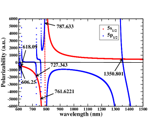
Figure 1: (color online) Magic wavelengths identified by arrows for the $5p_{1/2}-5s$ transition in Rb using the linearly polarized light.

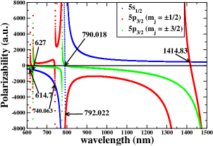
Figure 2: (color online) Magic wavelengths identified by arrows for the $5p_{3/2}-5s$ transition in Rb using the linearly polarized light.

Table 7: Comparison of the static and ac polarizabilities (in au) in Rb atom for the $5s$, $5p_{1/2}$ and $5p_{3/2}$ states with other experiments and theory.

	$\alpha^{0}_{5s}$	$\alpha^{0}_{5p_{1/2}}$	$\alpha^{0}_{5p_{3/2}}$	$\alpha^{2}_{5p_{3/2}}$
Present	318.3(6)	810.5(1.1)	868.0(1.7)	$-165.9(5)$
Other	317.39a	805d	867d	$-167^{d}$
Other	318.6(6)b	807e	870e	$-171^{e}$
Exp.	318.79(1.42)c	810.6(6)f	857(10)g	$-163(3)^{g}$

References:	a spol2
	b derevianko2
	c spol
	d arora1
	e poldere
	f hunter1 ; pol-andrei
	g krenn

IV.3 Status of the polarizability results

To affirm the broad interest of studying polarizabilities in Rb atom, we discuss briefly below about various experimental and theoretical works in the evaluation of polarizabilities of the $5s$ and $5p$ states reported so far in the Rb atom. There were several measurements carried out on Stark shifts in Rb atom almost two decades ago hunter1 ; hunter2 ; hunter3 ; tanner1 from which the polarizabilities of the $5s$ ground state and few excited states were estimated. Hunter and coworkers had observed the dc Stark shifts of the D1 line in Rb using a pair of cavity stabilized diode lasers locked to resonance signals hunter1 ; hunter2 ; hunter3 . In another work, Tanner and Wieman had used a crossed-beam laser spectroscopy with frequency stabilized laser diodes to measure the differential Stark shift of D2 line tanner1 . Marrus et al. had used a atomic beam method long ago to measure the Stark shift from which both the scalar and tensor polarizabilities of the $5p_{3/2}$ state were determined marrus .

Table 8: Magic wavelengths $\lambda_{\rm{magic}}$ for the linearly polarized light above 600 $nm$ for the $5p_{1/2}-5s$ and $5p_{3/2}-5s$ transitions in Rb and the corresponding values of polarizabilities at the magic wavelengths. The wavelengths (in vacuum) are given in $nm$ and polarizabilities are given in au. The given $m_{j}$ values correspond to the $5p$ states.

Transition: $5p_{1/2}~{}-~{}5s$
	$|m_{j}|$	$\lambda_{\rm{magic}}$	$\lambda_{\rm{magic}}$Ref. arora1	$\alpha(\lambda_{\rm{magic}})$
	1/2	606.25(1)	606.2(1)	$-443.3$
	1/2	618.09(2)	617.7(7)	$-490$
	1/2	727.343(2)	727.35(1)	$-1876$
	1/2	761.6221(2)	761.5(1)	$-5270$
	1/2	787.633(2)	787.6(1)	5382
	1/2	1350.801(9)	1350.9(5)	475.5
Transition: $5p_{3/2}~{}-~{}5s$
	$|m_{j}|$	$\lambda_{\rm{magic}}$	$\lambda_{\rm{magic}}$Ref. arora1	$\alpha(\lambda_{\rm{magic}})$
	1/2	614.70(1)	614.7(1)	$-477$
	3/2	626.62(3)	626.2(9)	$-529$
	1/2	627.70(1)	627.3(5)	$-534$
	1/2	740.063(2)	740.07(1)	$-2493$
	1/2	775.868(1)	775.84(1)	$-20030$
	3/2	775.8228(2)	775.77(3)	$-19917$
	3/2	790.018(2)	789.98(2)	53
	1/2	792.022(1)	792.00(1)	$-6973$
	1/2	1414.83(3)	1414.8(5)	455

The extensive calculation of polarizabilities in Rb atom was first carried out by Marinescu et al. using an $l$-dependent model potential marinescu . In this work, the infinite second-order sums in the polarizability calculations were transformed into integrals over the solutions of two coupled inhomogeneous differential equations and the integrals were carried out using Numerov integration method numerov . In 2004, Zhu et al. employed the RCC method to calculate the scalar and tensor polarizabilities of the ground and the first $p$ excited states in alkali atoms zhu . The results obtained using the RCC method were substantially improved over the earlier calculations based on the non-relativistic theories. Later, Arora et al. extended these calculations to obtain frequency-dependent scalar and tensor polarizabilities of the ground and first excited $5p$ states in Rb arora1 ; arora2 ; arora3 using the RCC method at the linearized singles, doubles and partial triples excitations level (SDpT method).

As has been discussed earlier, we have optimize at least seven important E1 matrix elements which are crucial in obtaining the polarizabilities of the $5s$ and $5p$ states and the other matrix elements have been obtained using the CCSD(T) method which includes all the non-linear terms. Therefore, the predicted polarizabilities of the $5s$ and $5p$ states obtained in this work are expected to be accurate enough to employ them further in the determination of the magic wavelengths in Rb atom, which is the prime motivation of the present work. In Table 7, we compare our polarizability results with the other reported values. Our results are more polished over the earlier studied results mainly due to the optimization of the matrix elements.

In our knowledge, there are no experimental and/or theoretical results on vector polarizabilities of the $5s$ and $5p$ states for any wavelengths available in Rb atom to compare with the present calculations. Accuracy in these polarizabilities will determine correct values of the magic wavelengths for the circularly polarized light in this atom. Since the E1 matrix elements required to determine the vector polarizabilities are same as required for the calculation of scalar and tensor polarizabilities, we expect a similar precision in our used vector polarizability results as discussed in the last subsection. We shall present the vector polarizabilities in the $5s$ and $5p$ states at a given wavelength (say close to a particular $\lambda_{\rm{magic}}$ value) so that if necessary our results can also be further verified by any other study.

Table 9: Contributions to the $5s$ scalar ($\alpha^{0}_{v}$) and vector ($\alpha^{1}_{v}$) polarizabilities at $\lambda$=770 $nm$ in Rb. Uncertainties in the results are given in the parentheses.

Contribution	$\alpha^{0}_{v}$	$\alpha^{1}_{v}$
$\alpha_{5s_{1/2}}(v)$
$5s_{1/2}\rightarrow 5p_{1/2}$	$-1576.1(2)$	$3254.4(4)$
$5s_{1/2}\rightarrow 6p_{1/2}$	0.515	$-0.565$
$5s_{1/2}\rightarrow 7p_{1/2}$	0.047	0.044
$5s_{1/2}\rightarrow 8p_{1/2}$	0.011	0.010
$5s_{1/2}\rightarrow 9p_{1/2}$	0.006	0.005
$5s_{1/2}\rightarrow 5p_{3/2}$	$-7615(1)$	$-7716(1)$
$5s_{1/2}\rightarrow 6p_{3/2}$	1.339	0.731
$5s_{1/2}\rightarrow 7p_{3/2}$	0.144	0.067
$5s_{1/2}\rightarrow 8p_{3/2}$	0.039	0.017
$5s_{1/2}\rightarrow 9p_{3/2}$	0.016	0.007
$\alpha_{5s_{1/2}}(c)$	9.2(5)	0.0
$\alpha_{5s_{1/2}}(vc)$	$-0.26(2)$	$\sim 0.0$
$\alpha_{\rm{tail}}$	0.14(1)	0.002(1)
Total	$-9180(1.1)$	$-4462(1.1)$

IV.4 AC Stark shifts and magic wavelengths

Following Eq. (6), the ac Stark shift $\Delta E_{v}$ of an atomic energy level $E_{v}$ due to the external applied ac electric field $\mathcal{E}$, in the absence of any magnetic field, can be parametrized in terms of $\alpha_{0}$, $\alpha_{1}$ and $\alpha_{2}$ as derevianko1

$$\Delta E_{v} = -\frac{1}{2}\mathcal{E}^{2}[\alpha_{v}^{0}(\omega)+\mathcal{A}\frac{m_{j}}{j_{v}}\alpha_{v}^{1}(\omega)$$ (26)

$$+\left(\frac{3m_{j}^{2}-j_{v}(j_{v}+1)}{j_{v}(2j_{v}-1)}\right)\alpha_{v}^{2}(\omega)]$$

In this formula, the frequency $\omega$ is assumed to be several line-widths off-resonance. The differential ac Stark shift for a transition is defined as the difference between the Stark shifts of individual levels. For instance, the interested differential ac Stark shifts in our case are for the $5p_{i}-5s$ transitions (with $i=1/2,3/2$) which are given by

$$\delta(\Delta E)_{5p_{i}-5s} = \Delta E_{5p_{i}}-\Delta E_{5s}$$ (27)

$$= \frac{1}{2}\mathcal{E}^{2}(\alpha_{5s}-\alpha_{5p_{i}}),$$

where we have used the total polarizabilities of the respective states. Since the external electric field $\mathcal{E}$ is arbitrary, we can verify the frequencies or wavelengths where $\alpha_{5p_{i}}=\alpha_{5s}$, for the null differential ac Stark shifts.

In order to estimate the total polarizability for any particular set of $j_{v}$ and $m_{j}$ values, we need to determine the scalar, vector and tensor polarizabilities. Magic wavelengths are calculated for a continuous values of frequencies (can also be expressed in terms of wavelength $\lambda$) by plotting the total polarizability for different states against the $\lambda$ values. The crossing between the two polarizabilities at various values of wavelengths will correspond to $\lambda_{\rm{magic}}$. Trapping of Rb atoms is convenient at these wavelengths as was stated in the beginning. As pointed out in arora1 , the linearly polarized lattice scheme offers only a few cases in which the magic wavelengths are suitable from the experimental point of view. Therefore, we would like to explore the idea of using the circularly polarized light for which the magic wavelengths need to be determined separately for each magnetic quantum number $m_{j}$.

Table 10: Contributions to the $5p_{1/2}$ scalar ($\alpha^{0}_{v}$) and vector ($\alpha^{1}_{v}$) polarizabilities at $\lambda$=770 $nm$ in Rb. Uncertainties in the results are given in the parentheses.

Contribution	$\alpha^{0}_{v}$	$\alpha^{1}_{v}$
$\alpha_{5p_{1/2}}(v)$
$5p_{1/2}\rightarrow 5p_{1/2}$	1567.1(2)	3254.4(4)
$5p_{1/2}\rightarrow 6s_{1/2}$	$-85.029(5)$	292.38(2)
$5p_{1/2}\rightarrow 7s_{1/2}$	46.676(4)	$-88.283(7)$
$5p_{1/2}\rightarrow 8s_{1/2}$	3.020	$-4.764$
$5p_{1/2}\rightarrow 9s_{1/2}$	0.954	$-1.382$
$5p_{1/2}\rightarrow 10s_{1/2}$	0.412	$-0.570$
$5p_{1/2}\rightarrow 4d_{3/2}$	$-262.99(1)$	$-504.00(2)$
$5p_{1/2}\rightarrow 5d_{3/2}$	382.94(2)	379.02(2)
$5p_{1/2}\rightarrow 6d_{3/2}$	13.029(1)	10.504(1)
$5p_{1/2}\rightarrow 7d_{3/2}$	5.035(2)	3.694(2)
$5p_{1/2}\rightarrow 8d_{3/2}$	2.565(1)	1.787(1)
$5p_{1/2}\rightarrow 9d_{3/2}$	1.413	0.954
$\alpha_{5p_{1/2}}(c)$	9.2(5)	0.0
$\alpha_{5p_{1/2}}(vc)$	$\sim 0.0$	$\sim 0.0$
$\alpha_{\rm{tail}}$	17.6(20)	3.8(4)
Total	1711(2)	3347.7(4)

In the next two subsections, we shall discuss about the magic wavelengths for the $5p_{1/2,3/2}-5s$ transitions for both the linearly and circularly polarized lights. The reason for bringing up the issue of magic wavelengths for the linearly polarized lights in these transitions is that since we have obtained the most accurate results for all the static polarizabilities it is expected that we will get better results for the magic wavelengths using our optimized set of E1 matrix elements. This will also help us in making a comparison study between the results obtained from the linearly and circularly polarized lights.

IV.5 Case for the linearly polarized optical traps

Since we are interested in optical traps and the previous study arora1 reveals that the magic wavelengths for the $5s-5p$ transitions at which the Rb atom can be trapped using the linearly polarized lights lie in between $600-1500\ nm$, we try to find out the null differential polarizabilities in this region. In Fig. 1, we plot the total polarizabilities due to the linearly polarized lights for both the $5s$ and $5p_{1/2}$ states. As seen in the figure, the $5s$ state dynamic polarizabilities are generally small in this region except for the wavelengths in close vicinity to the $5s-5p_{1/2}$ resonance (at 795 $nm$) and $5s-5p_{3/2}$ resonance (at 780 $nm$). However, the $5p_{1/2}$ state has several resonances in the considered wavelength range. It is generally expected that the $5p_{1/2}$ state polarizability will cross the $5s$ state polarizability in between each pair of resonances. We found total six magic wavelengths for the $5p_{1/2}\rightarrow 5s$ transition in between the five resonances.

Table 11: Contributions to the $5p_{3/2}$ scalar ($\alpha^{0}_{v}$) and vector ($\alpha^{1}_{v}$) and tensor ($\alpha^{2}_{v}$) polarizabilities at $\lambda$=770 $nm$ in Rb. Uncertainties in the results are given in the parentheses.

Contribution	$\alpha^{0}_{v}$	$\alpha^{1}_{v}$	$\alpha^{2}_{v}$
$\alpha_{5p_{3/2}}(v)$
$5p_{3/2}\rightarrow 5s_{1/2}$	3807.5(7)	11575(2)	$-3807.5(7)$
$5p_{3/2}\rightarrow 6s_{1/2}$	$-85.017(9)$	452.76(5)	85.017(9)
$5p_{3/2}\rightarrow 7s_{1/2}$	68.181(6)	$-196.85(2)$	$-68.181(6)$
$5p_{3/2}\rightarrow 8s_{1/2}$	3.194	$-7.667(1)$	$-3.194$
$5p_{3/2}\rightarrow 9s_{1/2}$	0.984	$-2.168$	$-0.984$
$5p_{3/2}\rightarrow 10s_{1/2}$	0.422	$-0.885$	$-0.422$
$5p_{3/2}\rightarrow 4d_{3/2}$	$-25.311(5)$	60.32(1)	$-20.249(4)$
$5p_{3/2}\rightarrow 5d_{3/2}$	$-61.57(1)$	74.47(1)	$-49.25(1)$
$5p_{3/2}\rightarrow 6d_{3/2}$	1.607(1)	$-1.578(1)$	1.286(1)
$5p_{3/2}\rightarrow 7d_{3/2}$	0.591	$-0.527$	0.473
$5p_{3/2}\rightarrow 8d_{3/2}$	0.293	$-0.248$	0.234
$5p_{3/2}\rightarrow 9d_{3/2}$	0.162	$-0.133$	0.130
$5p_{3/2}\rightarrow 4d_{5/2}$	$-225.3(2)$	$-805.4(6)$	45.06(4)
$5p_{3/2}\rightarrow 5d_{5/2}$	$-564.1(3)$	$-1023.3(6)$	112.8(1)
$5p_{3/2}\rightarrow 6d_{5/2}$	14.06(1)	20.70(1)	$-2.811(2)$
$5p_{3/2}\rightarrow 7d_{5/2}$	5.264(2)	7.046(3)	$-1.053$
$5p_{3/2}\rightarrow 8d_{5/2}$	2.597(1)	3.298(1)	$-0.519$
$5p_{3/2}\rightarrow 9d_{5/2}$	1.2700	1.562	$-0.254$
$\alpha_{5p_{3/2}}(c)$	9.3(5)	0.0	0.0
$\alpha_{5p_{3/2}}(vc)$	$\sim 0.0$	$\sim 0.0$	$\sim 0.0$
$\alpha_{\rm{tail}}$	19(2)	6.9(7)	$-4.7(9)$
Total	2973(2)	10163(5)	$-3714(1)$

However, the case for the $5p_{3/2}\rightarrow 5s$ transition is different owing to the presence of non-zero tensor contribution of the $5p_{3/2}$ state. As shown in Fig. 2, we get different magic wavelengths for the $5p_{3/2}\rightarrow 5s$ transition at $m_{j}=\pm 1/2$ and $m_{j}=\pm 3/2$ sub-levels of the $5p_{3/2}$ state. There are few wavelengths in between resonances where $\alpha_{5p_{3/2}}$ with $m_{j}=\pm 3/2$ contribution is not same as the $\alpha_{5s}$. This leads to reduction in the number of magic wavelengths for this transition. For example, we did not find any $\lambda_{\rm{magic}}$ between the $5p_{3/2}-4d_{3/2,5/2}$ resonances (at 1529 $nm$) and the $5p_{3/2}-6s$ resonance (at 1367 $nm$) for $m_{j}=\pm 3/2$ sublevels of the $5p_{3/2}$ state.

We have limited our search for the magic wavelengths where the differential polarizabilities between the $5s$ and $5p_{j}$ states are less than 0.5%. Based on all these data, we list now $\lambda_{\rm{magic}}$ (in vacuum) above 600 $nm$ in Table 8 for the $5p_{1/2}-5s$ and $5p_{3/2}-5s$ transitions in Rb atom and compare them with the previously known results. The present results are improved slightly due to the optimized E1 matrix elements used here. The uncertainties in our magic wavelength results are found as the maximum differences between the $\alpha_{5s}\pm\delta\alpha_{5s}$ and $\alpha_{5p}\pm\delta\alpha_{5p}$ contributions with their respective magnetic quantum numbers, where the $\delta\alpha$ are the uncertainties in the polarizabilities for their corresponding states.

The reason for not acquiring sufficient number of magic wavelengths for the $5p_{3/2}-5s$ transition lies in the fact that extra contribution from the tensor polarizability to the total $5p_{3/2}$ polarizability is not compensated by the counter part of the $5s$ state. The idea of using the circularly polarized light to obtain magic wavelengths for the $5p_{3/2}-5s$ transition is triggered from that fact that the extra contribution from the tensor polarizability to the $5p_{3/2}$ state might be cancelled by the vector polarizability contributions or the vector polarizabilities are so large that they may play a dominant role in determining the differential polarizabilities. This would be evident in the following subsection.

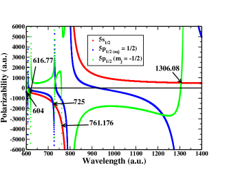
Figure 3: (color online) Magic wavelengths identified by arrows for the $5p_{1/2}-5s$ transition in Rb using the left-handed circularly polarized light.

Table 12: Magic wavelengths $\lambda_{\rm{magic}}$ above 600 $nm$ for the $5p_{1/2}-5s$ transition in Rb and the corresponding values of total polarizabilities at the magic wavelengths for the left-circularly polarized laser beam. The wavelengths (in vacuum) are given in $nm$ and polarizabilities are given in au. The given $m_{j}$ values are for the $5p$ states.

Transition: $5p_{1/2}~{}-~{}5s$
$m_{j}$	$\lambda_{\rm{magic}}$	$\alpha(\lambda_{\rm{magic}})$	$\lambda_{\rm{magic}}(\rm{avg})$
1/2	600.83(14)	$-405$
			604(7)
-1/2	607.98(1)	-428
-1/2	616.77(2)	$-461$	617
1/2	721.628(23)	$-1449$
			725(7)
-1/2	728.843(1)	-1633
-1/2	761.176(1)	$-3424$	761
-1/2	1306.08(1)	504	1306

Table 13: Magic wavelengths $\lambda_{\rm{magic}}$ above 600 $nm$ for the $5p_{3/2}-5s$ transition in Rb and the corresponding values of total polarizabilities at the magic wavelengths for the left-circularly polarized laser beam. The wavelengths (in vacuum) are given in $nm$ and polarizabilities are given in au. The given $m_{j}$ values are for the $5p$ states.

Transition: $5p_{3/2}~{}-~{}5s$
$m_{j}$	$\lambda_{\rm{magic}}$	$\alpha(\lambda_{\rm{magic}})$	$\lambda_{\rm{magic}}(\rm{avg})$
1/2	613.25(3)	$-447$
-1/2	615.51(1)	$-456$	616(5)
-3/2	618.15(2)	$-466$
3/2	630.142(1)	$-516$
1/2	628.30(1)	$-508$
			628(5)
-1/2	626.95(1)	$-502$
-3/2	625.04(3)	$-494$
3/2	746.737(15)	$-2328$
1/2	738.794(32)	$-1964$
			742(8)
-1/2	740.587(1)	$-2037$
-3/2	742.262(1)	$-2109$
3/2	775.836(5)	$-6231$
1/2	775.834(7)	$-6230$
			775.8(2)
-1/2	775.789(3)	$-6215$
-3/2	775.693(2)	$-6183$
1/2	783.883(13)	$-10925$
-1/2	787.547(4)	$-16431$	786(4)
-3/2	776.497(4)	$-16318$
1/2	1454.4(9)	453
-1/2	1387.1(1)	473	1382(149)
-3/2	1305.9(1)	504

IV.6 Case for the circularly polarized optical traps

As mentioned previously, polarizabilities for the circularly polarized light have extra contribution from the vector component of the tensor product between the dipole operators. This extra factor is expected to provide better results for state-insensitive trapping. First, we present the scalar, vector and tensor dynamic polarizabilities of the $5s$, $5p_{1/2}$ and $5p_{3/2}$ states in Tables 9, 10 and 11, respectively, at $\lambda=770\ nm$ to perceive their general behavior. The choice of this wavelength is deliberate for being close to one of the magic wavelengths for the circularly polarized light (e.g. see Table (12) and (13)). Hereafter we shall consider the left-handed circularly polarized light for all the practical purposes as the results will have a similar trend with the right-handed circularly polarized light due to the linear dependency of degree of polarizability $\mathcal{A}$ in Eq. (26). Nevertheless, the left or right handed polarization in the experimental set up is just a matter of choice.

For the sake of completeness of our study, we also search for magic wavelengths in the $5s-5p_{1/2}$ transition in Rb atoms using the circularly polarized light although a fairly large number of magic wavelengths for this transition is found using the linearly polarized light. For this purpose, we plot net dynamic polarizability results of the $5s$ and $5p_{1/2}$ states in Fig. 3 using the circularly polarized light against different values of wavelength. The figure shows that the total polarizability of the $5s$ state for any values of $\lambda$ is very small except for the wavelengths close to the two primary resonances. Due to the $m_{j}$ dependence of the vector polarizability coefficient in Eq. (26), the crossing occurs at a different wavelength for the different values of $m_{j}$ in between two $5p_{1/2}$ resonances. As shown in Table 12, we get set of five magic wavelengths in between seven $5p_{1/2}$ resonances lying in the wavelength range 600-1400 $nm$. Out of these five sets of magic wavelengths three sets of the magic wavelengths occur only for negative values of $m_{j}$. Thus, the number of convenient magic wavelengths for the above transition is less than the number of magic wavelengths obtained for the linearly polarized light. This advocates for the use of linearly polarized light in this transition, though choice of the circularly polarized light is not bad at all. The $m_{j}$ dependence of traps and the difficulties in building a viable experimental set up in the case of circularly polarized light could be the other major concern.

In this work, we also propose the use of ”switching trapping scheme” (described below) which may solve the problem in cases where state-insensitive trapping is only supportive for the negative $m_{j}$ sublevels of $5p$ states. We observed that the same magic wavelength will support state-insensitive trapping for negative $m_{j}$ sublevels if we switch the sign of $\mathcal{A}$ and $m_{j}$ of $5s$ state. In other words, the change of sign of $\mathcal{A}$ and $m_{j}$ sublevels of $5s$ state will lead to the same result for the positive values of $m_{j}$ sub-levels of $5p$ states.

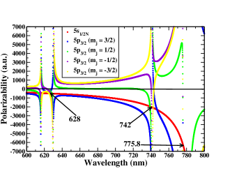
Figure 4: (color online) Magic wavelengths identified by arrows for the $5p_{3/2}-5s$ transition in Rb using the left-handed circularly polarized light.

Here we give more emphasis on finding more magic wavelengths for the $5s-5p_{3/2}$ transition which can be used in the state-insensitive trapping scheme for the Rb atom. In Table 13, we list a number of $\lambda_{\rm{magic}}$ for the $5s-5p_{3/2}$ transition in the far-optical and near infrared wavelengths along with the uncertainties in the $\lambda_{\rm{magic}}$ and the polarizabilities at the $\lambda_{\rm{magic}}$ values. We also list the $\lambda_{\rm{magic}}(\rm{avg})$ values in the table which are the average of the magic wavelengths at different $m_{j}$ sublevels. The error in the $\lambda_{\rm{magic}}(\rm{avg})$ is calculated as the maximum difference between the magic wavelengths from different $m_{j}$ sublevels. For this transition we get a set of six magic wavelengths in between seven $5p_{3/2}$ resonances lying in the wavelength range 600-1400 $nm$ (i.e. $5p_{3/2}-4d_{j}$ resonance at 1529 $nm$, $5p_{3/2}-6s$ resonance at 1367 $nm$, $5p_{3/2}-5s$ resonance at 780 $nm$, $5p_{3/2}-5d_{j}$ resonance at 776 $nm$, $5p_{3/2}-7s$ resonance at 741 $nm$, $5p_{3/2}-6d_{j}$ resonance at 630 $nm$, and $5p_{3/2}-8s$ resonance at 616 $nm$). Five out of six magic wavelengths support a blue detuned trap (predicted by the negative values of dynamic polarizability). Out of these five magic wavelengths the magic wavelength at 628 $nm$ and 742 $nm$ are recommended for blue detuned traps. The magic wavelength at 742 $nm$ supports a stronger trap (as shown by a larger value of the polarizability at this wavelength in Fig.(4)). The magic wavelength at 775.8 $nm$ is very close to the resonance and might not be useful for practical purposes. The magic wavelength at 1382 $nm$ supports a red detuned optical trap. It can be observed from Table 13 that $m_{j}=3/2$ sublevel does not support state-insensitive trapping at this wavelength. However, using a switching trapping scheme as described in the previous paragraph will allow trapping this sublevel too. The magic wavelength at 1382 $nm$ is recommended owing to the fact that it is not close to any atomic resonance and supports a red-detuned trap which was not found in the linearly polarized trapping scheme.

V summary

In conclusion, we have employed the relativistic coupled cluster method in the singles, doubles and triples excitations approximation to determine the electric dipole matrix elements in rubidium atom. Some of the important matrix elements were further optimized using the experimental lifetimes of few excited states and static polarizabilities of the ground and $5p_{1/2,3/2}$ excited states. These optimized matrix elements were then used to improve the precision of the available lifetime results for some of the low-lying excited states in the considered atom. We also observe disagreement between our calculated dynamic polarizability with a measurement at the wavelength 1064 $nm$ using the above optimized matrix elements.

We have compared the static and dynamic polarizability results from various works and reported the improved values of the magic wavelengths for the $5s\rightarrow 5p_{1/2}$ transition using the linearly polarized light. Issues related to state-insensitive trapping of rubidium atoms for the $5s\rightarrow 5p_{3/2}$ transition with linearly polarized light are discussed and use of the circularly polarized light is emphasized. Finally, we evaluate six set of magic wavelengths for the $5s\rightarrow 5p_{3/2}$ transition which can be used for the above purpose out of which we have recommended two magic wavelengths at 628 $nm$ and 742 $nm$ for the blue detuned optical traps and 1382 $nm$ for the red detuned optical traps. We also proposed the use of a switching trapping scheme for the magic wavelengths at which the state-insensitive trapping is supported only for either positive or negative $m_{j}$ sublevels of $5p$ states.

References

- (1) A. Godone, F. Levi, S. Micalizio, E. K. Bertacco and C. E. Calosso, IEEE Transactions on Instrumentation and Measurement 56, 378 (2007).
- (2) J. Vanier and C. Mandache, Appl. Phys. B 87, 565 (2007).
- (3) B. Butscher, J. Nipper, J. B. Balewski, L. Kukota, V. Bendkowsky, R. Low and T. Pfau, Nat. Phys. 6, 970 (2012).
- (4) X. L. Zhang, L. Ishenhower, A. T. Gill, T. G. Walker and M. Saffman, Phys. Rev. A 82, 030306 (2010).
- (5) Y. O. Dudin, A. G. Radnaev, R. Zhao, J. Z. Blumoff, T. A. B. Kennedy and A. Kuzmich, Phys. Rev. Lett. 105, 260502 (2010).
- (6) S. Tassy, N. Nemitz, F. Baumer, C. Hohl, A. Batar and A. Gorlitz, J. Phys. B 43, 205309 (2010).
- (7) J. Guena, P. Rosenbusch, P. Laurent, M. Abgrall, D. Rovera, G. Santarellu, M. E. Tobar, S. Bize and A. Clairon, IEEE Trans. on Ultrasonics, Ferroelectrics, and Frequency Control 57, 647 (2010).
- (8) H. Marion, F. P. D. Santos, M. Abgrall, S. Zhang, Y. Sortais, S. Bize, I. Maksimovic, D. Calonico, J. Grunert, C. Mandache et al., Phys. Rev. Lett. 90, 15801 (2003).
- (9) International Committee for Weights and Measures, Proceedings of the sessions of the 95th meeting (October 2006); http://www.bipm.org/utils/en/pdf/CIPM2006-EN.pdf
- (10) D. Sheng, L. A. Orozco and E. Gomez, J. Phys. B 43, 074004 (2010).
- (11) H. S. Nataraj, B. K. Sahoo, B. P. Das and D. Mukherjee, Phys. Rev. Lett. 101, 033002 (2008).
- (12) C. E. Theodosiou, Phys. Rev. A 30, 2881 (1984).
- (13) W. A. van Wijngaarden and J. Sagle, Phys. Rev. A 45, 1502 (1992).
- (14) E. Gomez, F. Baumer, A. D. Lange, G. D. Sprouse and L. A. Orozco, Phys. Rev. A 72, 012502 (2005).
- (15) D. Sheng, A. P. Galvan and L. A. Orozco, Phys. Rev. A 78, 062506 (2008).
- (16) J. Marek and P. Munster, J. Phys. B 13, 1731 (1980).
- (17) C. Tai, W. Happer and R. Gupta, Phys. Rev. A 12, 736 (1975).
- (18) M. S. Safronova and U. I. Safronova, Phys. Rev. A 83, 052508 (2011).
- (19) J. Walls, J. Clarke, S. Cauchi, G. Karkas, H. Chen and W. A. van Wijngaarden, Eur. Phys. J. D 14, 9 (2001).
- (20) H.-C. Chui, M.-S. Ko, Y.-W. Liu, J.-T. Shy, J.-L. Peng and H. Ahn, Opt. Lett. 30, 842 (2005).
- (21) A. P. Calvan, Y. Zhaoa, L. A. Orozco, E. Gomez, A. D. Lange, F. Baumer and G. D. Sprouse, Phys. Lett. B 655, 114 (2007).
- (22) N. Schlosser, G. Reymond, I. Protsenko and P. Grangier, Nature 411, 1024 (2001).
- (23) S. Kuhr, W. Alt, D. Schrader, M. Muller, V. Gomer and D. Meschede, Science 293, 278 (2001).
- (24) H. Katori, Proceedings of the Sixth Symposium Frequency Standards and Metrology, ed. by P. Gill, World Scientific Singapore, p. 323 (2002).
- (25) C. A. Sackett, D. Kielpinski, B. E. King, C. Langer, V. Meyer, C. J. Myatt, M. Rowe, Q. A. Turchette, W. M. Itano, D. J. Wineland and C. Monroe, Nature 404, 256 (2006).
- (26) M. S. Safronova, C. J. Williams and C. W. Clark, Phys. Rev. A 67, 040303(R) (2003).
- (27) M. Takamoto and H. Katori, Phys. Rev. Lett. 91, 223001 (2003).
- (28) H. Katori, T. Ido and M. Kuwata-Gonokami, J. Phys. Soc. Jpn 68, 2479 (1999).
- (29) A. D. Ludlow et al. et al., Science 319, 1805 (2005).
- (30) J. McKeever, J. R. Buck, A. D. Boozer, A. Kuzmich, H.-C. Nagerl, D. M. Stamper-Kurn and H. J. Kimble, Phys. Rev. Lett. 90, 133602 (2003).
- (31) Bindiya Arora, M. S. Safronova and C. W. Clark, Phys. Rev. A 76, 052509 (2007).
- (32) V. V. Flambaum, V. A. Dzuba and A. Derevianko, Phys. Rev. Lett. 101, 220801 (2008).
- (33) C. Y. Park, H. Noh, C. M. Lee and D. Cho, Phys. Rev. A 63, 032512 (2001).
- (34) Keith D. Bonin and Vitaly V. Kresin, Electric-dipole Polarizabilities of Atoms, Molecules and Clusters, World Scientific Publishing Co. Pte Ltd (1997).
- (35) N. L. Manakov, V. D. Ovsiannikov and L. P. Rapoport, Physics Rep. 141, 319 (1986).
- (36) I. Lindgren, Int. J. Quantum Chem. 12, 33 (1978).
- (37) B. K. Sahoo, B. P. Das, R. K. Chaudhuri and D. Mukhrejee, J. Comput. Methods Sci. Eng. 7, 57 (2007).
- (38) Bindiya Arora, D. Nandy and B. K. Sahoo, Phys. Rev. A 85, 02506 (2012).
- (39) C. E. Moore, Atomic Energy Levels, U.S. GPO, Washington, D.C., Natl. Bur. Stand. (U.S.), Natl. Bur. Stand. Ref. Data Ser., ”U.§. Govt. Print. Off., v. 35 (1971).
- (40) Yu. Ralchenko, F. -C. Jou, D. E. Kelleher, A. E. Kramida, A. Musgrove, J. Reader, W. L. Wiese and K. Olsen, NIST Atomic Spectra Database, (version 3.1.2), National Institute of Standards and Technology, Gaithersburg, MD (2005).
- (41) J. E. Sansonetti, W. C. Martin and S.L. Young, Handbook of Basic Atomic Spectroscopic Data, (version 1.1.2), National Institute of Standards and Technology, Gaithersburg, MD (2005).
- (42) B. K. Sahoo, B. P. Das and D. Mukherjee, Phys. Rev. A 79, 052511 (2009).
- (43) D. Mukherjee, B. K. Sahoo, H. S. Nataraj and B. P. Das, J. Phys. Chem. A 113, 12549 (2009).
- (44) B. K. Sahoo, S. Majumder, R. K. Chaudhuri, B. P. Das and D. Mukhrejee, J. Phys. B 37, 3409 (2004).
- (45) R. W. Schmieder, A. Lurio and W. Happer, Phys. Rev. A 3, 1209 (1971).
- (46) M. Marinescu, H. R. Sadeghpour and A. Dalgarno, Phys. Rev. A 49, 5103 (1994).
- (47) C. Zhu, A. Dalgarno, S. G. Porsev and A. Derevianko, Phys. Rev. A 70, 03722 (2004).
- (48) M. S. Safronova, Bindiya Arora and C. W. Clark, Phys. Rev. A 73, 022505 (2006).
- (49) R. F. Gutterres, C. Amiot, A. Fioretti, C. Gabbanini, M. Mazzoni and O. Dulieu, Phys. Rev. A 66, 024502 (2002).
- (50) W. F. Holmgren, M. C. Revelle, V. P. A. Lonij and A. D. Cronin, Phys. Rev. A 81, 053607 (2010).
- (51) W. R. Johnson, D. Kolb and K.-N. Huang, At. Data Nucl. Data Tables 28, 334 (1983).
- (52) K. D. Bonin and M. A. Kadar-Kallen, Phys. Rev. A 47, 944 (1993).
- (53) K. E. Miller, D. Krause and L. R. Hunter, Phys. Rev. A 49, 5128 (1994).
- (54) J. Marek and P. Münster, J. Phys. B: Atom. Molec. Phys. 13, 1731 (1980).
- (55) C. Krenn, W. Scherf, O. Khait, M. Musso and L. Windholz, Z. Phys. D:At. Mol. Clusters 41, 229 (1997).
- (56) L. R. Hunter, D. Krause, S. Murthy and T. W. Sung, Phys. Rev. A 37, 3283 (1988).
- (57) L. R. Hunter, D. Krause, K. E. Miller, D. J. Berkeland and M. G. Boshier, Optics Comm. 94, 2010 (1992).
- (58) C. Tanner and C. Wieman, Phys. Rev. A 38, 162 (1988).
- (59) R. Marrus, D. McColm and J. Yellin, Phys. Rev. A 147, 55 (1966).
- (60) M. J. Seaton, Comp. Phys. Comm. 146, 254 (2002).
- (61) Bindiya Arora, M. S. Safronova and C. W. Clark, Phys. Rev. A 76, 052516 (2007).
- (62) M. S. Safronova, W. R. Johnson and A. Derevianko, Phys. Rev. A 60, 4476 (1999).
- (63) A. Derevianko, W. R. Johnson, M. S. Safronova and J. F. Babb, Phys. Rev. Lett. 82, 3589 (1999).
- (64) Cheng Zhu, Alex Dalgarno, Sergey G. Porsev and Andrei Derevianko, Phys. Rev. A 70, 032722 (2004).
- (65) A. Derevianko, W. R. Johnson, M. S. Safronova and J. F. Babb, Phys. Rev. Lett. 82, 3589 (1999).