A Dynamical Analysis of the Proposed Circumbinary HW Virginis Planetary System

Abstract

In 2009, the discovery of two planets orbiting the evolved binary star system HW Virginis was announced, based on systematic variations in the timing of eclipses between the two stars. The planets invoked in that work were significantly more massive than Jupiter, and moved on orbits that were mutually crossing - an architecture which suggests that mutual encounters and strong gravitational interactions are almost guaranteed.

In this work, we perform a highly detailed analysis of the proposed HW Vir planetary system. First, we consider the dynamical stability of the system as proposed in the discovery work. Through a mapping process involving 91,125 individual simulations, we find that the system is so unstable that the planets proposed simply cannot exist, due to mean lifetimes of less than a thousand years across the whole parameter space.

We then present a detailed re-analysis of the observational data on HW Vir, deriving a new orbital solution that provides a very good fit to the observational data. Our new analysis yields a system with planets more widely spaced, and of lower mass, than that proposed in the discovery work, and yields a significantly greater (and more realistic) estimate of the uncertainty in the orbit of the outermost body. Despite this, a detailed dynamical analysis of this new solution similarly reveals that it also requires the planets to move on orbits that are simply not dynamically feasible.

Our results imply that some mechanism other than the influence of planetary companions must be the principal cause of the observed eclipse timing variations for HW Vir. If the system does host exoplanets, they must move on orbits differing greatly from those previously proposed. Our results illustrate the critical importance of performing dynamical analyses as a part of the discovery process for multiple-planet exoplanetary systems.

1 Introduction

Since the discovery of the first planets around other stars (Wolszczan & Frail, 1992; Mayor & Queloz, 1995), the search for exoplanets has blossomed to become one of the most exciting fields of modern astronomical research. The great majority of the hundreds of exoplanets that have been discovered over the past two decades have been found orbiting Sun-like stars by dedicated international radial velocity programs. Among these programmes are HARPS (the High Accuracy Radial velocity Planetary Search project, e.g. Pepe et al., 2004; Udry et al., 2007; Mayor et al., 2009), AAPS (the Anglo-Australian Planet Search, e.g. Tinney et al., 2001, 2011; Wittenmyer et al., 2012b), California (e.g. Howard et al., 2010; Wright et al., 2011), Lick-Carnegie (e.g. Rivera et al., 2010; Anglada-Escudé et al., 2012), and Texas (e.g. Endl et al., 2006; Robertson et al., 2012a). The other main method for exoplanet detection is the transit technique, which searches for the small dips in the brightness of stars that result from the transit of planets across them. Ground-based surveys such as WASP (Hellier et al., 2011; Smith et al., 2012) and HAT (Bakos et al., 2007; Howard et al., 2012) have pioneered such observations, and resulted in the discovery of a number of interesting planetary systems. In the coming years, such surveys using space-based observatories will revolutionise the search for exoplanets. Indeed, a rapidly growing contribution to the catalogue of known exoplanets comes from the Kepler spacecraft (e.g. Borucki et al., 2011; Welsh et al., 2012; Doyle et al., 2011), which will likely result in the number of known exoplanets growing by an order of magnitude in the coming years.

In recent years, a number of new exoplanet discoveries have been announced featuring host stars that differ greatly from the Sun-like archetype that make up the bulk of detections. The most striking of these are the circumbinary planets, detected around eclipsing binary stars via the periodic variations in the timing of observed stellar eclipses. A number of these unusual systems feature cataclysmic variable stars, interacting binary stars composed of a white dwarf primary and a Roche lobe filling M star secondary. Sharply-defined eclipses of the bright accretion spot, with periods of hours, can be timed with a precision of a few seconds. In these systems, the eclipse timings are fitted with a linear ephemeris, and the residuals ($O-C$) are found to display further, higher-order variations. These variations can be attributed to the gravitational effects of distant orbiting bodies which tug on the eclipsing binary stars, causing the eclipses to appear slightly early or late. This light-travel time (LTT) effect can then be measured and used to infer the presence of planetary-mass companions around these highly unusual stars. Some examples of circumbinary companions discovered in this manner include UZ For (Potter et al., 2011), NN Ser (Beuermann et al., 2010), DP Leo (Qian et al., 2010), HU Aqr (Schwarz et al., 2009; Qian et al., 2011) and SZ Her (Hinse et al., 2012b; Lee et al., 2012)

The first circumbinary planets to be detected around hosts other than pulsars were those in the HW Vir system (Lee et al., 2009), which features a subdwarf primary, of spectral class B, and a red dwarf companion which display mutual eclipses with a period of around 2.8 hours (Menzies & Marang, 1986). The detection of planets in this system was based on the timing of mutual eclipses between the central stars varying in a fashion that was best fit by including two sinusoidal timing variations. The first, attributed to a companion of mass $M~{}\sin~{}i\!=\!19.2~{}$M_Jup, had a period of 15.8 years, and a semi-amplitude of 77 s, while the second, attributed to a companion of mass $M~{}\sin~{}i\!=\!8.5~{}$M_Jup, had a period of 9.1 years and semi-amplitude of 23 s. Whilst these semi-amplitudes might appear relatively small, the precision with which the timing of mutual eclipses between the components of the HW Vir binary can be measured means that such variations are relatively easy to detect.

Over the last decade, a number of studies have shown that, for systems that are found to contain more than one planetary body, a detailed dynamical study is an important component of the planet discovery process that should not be overlooked (e.g. Stepinski et al., 2000; Goździewski & Maciejewski, 2001; Ferraz-Mello et al., 2005; Laskar & Correia, 2009). However, despite these pioneering works, the great majority of exoplanet discovery papers still fail to take account of the dynamical behaviour of the proposed systems. Fortunately, this situation is slowly changing, and recent discovery papers such as Robertson et al. (2012a), Wittenmyer et al. (2012b) and Robertson et al. (2012b) have shown how studying the dynamical interaction between the proposed planets can provide significant additional constraints on the plausible orbits allowed for those planets. Such studies can even reveal systems in which the observed signal cannot be explained by the presence of planetary companions. The planets proposed to orbit HU Aqr are one such case, with a number of studies (e.g. Horner et al., 2011; Funk et al., 2011; Hinse et al., 2012a; Wittenmyer et al., 2012a; Goździewski et al., 2012) showing that the orbital architectures allowed by the observations are dynamically unstable on astronomically short timescales. In other words, whilst it is clear that the observed signal is truly there, it seems highly unlikely that it is solely the result of orbiting planets.

Given these recent studies, it is clearly important to consider whether known multiple-planet exoplanetary systems are truly what they seem to be. In this work, we present a re-analysis of the 2-planet system proposed around the eclipsing binary HW Vir. In section 2, we briefly review the HW Vir planetary system as proposed by Lee et al. (2009). In section 3, a detailed dynamical analysis of the planets proposed in that work is performed. In section 4, we present a re-analysis of the observations of HW Vir that led to the announcements of the exoplanets, obtaining a new orbital solution for those planets which is dynamically tested in section 5. Finally, in section 6, we present a discussion of our work, and draw conclusions based on the results herein.

2 The HW Vir planetary system

The HW Vir system consists of a subdwarf B primary and an M6-7 main sequence secondary. The system eclipses with a period of 2.8 hours (Menzies & Marang, 1986), and the stars have masses of $M_{1}=0.48$ M_⊙ and $M_{2}=0.14$ M_⊙ (Wood & Saffer, 1999). Changes in the orbital period of the eclipsing binary were first noted by Kilkenny et al. (1994); further observations led other authors to suggest that the period changes were due to LTT effects arising from an orbiting substellar companion (Kilkenny et al., 2003; İbanoǧlu et al., 2004). Lee et al. (2009) obtained a further 8 years of photometric observations of HW Vir. Those data, in combination with the previously published eclipse timings spanning 24 years, indicated that the period changes consisted of a quadratic trend plus two sinusoidal variations with periods of 15.8 and 9.1 years. Lee et al. (2009) examined alternative explanations for the cyclical changes, ruling out apsidal motion and magnetic period modulation via the Applegate mechanism (Applegate, 1992). They concluded that the most plausible cause of the observed cyclic period changes is the light-travel time effect induced by two companions with masses 19.2 and 8.5 M_Jup. The parameters of their fit can be found in Table 1. Formally, the planets are referred to as HW Vir (AB)b and HW Vir (AB)c, but for clarity, we refer to the planets as HW Vir b and HW Vir c.

Parameter	HW Vir b	HW Vir c	Unit
$M~{}\sin~{}i$	0.00809 $\pm$ 0.00040	0.01836 $\pm$ 0.000031	$M_{\odot}$
$a~{}\sin~{}i$	3.62 $\pm$ 0.52	5.30 $\pm$ 0.23	AU
$e$	0.31 $\pm$ 0.15	0.46 $\pm$ 0.05
$\omega$	60.6 $\pm$ 7.1	90.8 $\pm$ 2.8	deg
$T$	2,449,840 $\pm$ 63	2,454,500 $\pm$ 39	HJD
$P$	3316 $\pm$ 80	5786 $\pm$ 51	days

Table 1: Parameters for the two planetary bodies proposed in the HW Vir system, taken from Lee et al. (2009) (their Table 7).

A first look at the fitted parameters for the two proposed planets reveals an alarming result: the planets are both massive, in the regime that borders gas giants and brown dwarfs, and occupy highly eccentric, mutually crossing orbits with separations that guarantee close encounters - generally a surefire recipe for dynamical instability (as seen for the proposed planetary system around HU Aqr (e.g. Horner et al., 2011; Hinse et al., 2012a; Wittenmyer et al., 2012a; Goździewski et al., 2012).

3 A dynamical search for stable orbits

The work by Lee et al. (2009) derived relatively high masses (8.5 and 19.2 M_Jup) and orbital eccentricities (0.31 and 0.46), and so significant mutual gravitational interactions are expected. To assess the dynamical stability of the proposed planets in the HW Vir system, we performed a large number of simulations of the planetary system, following a successful strategy used on a number of previous studies (e.g. Marshall et al., 2010; Horner et al., 2011; Wittenmyer et al., 2012a, b; Robertson et al., 2012a, b; Horner et al., 2012). We used the Hybrid integrator within the n-body dynamics package MERCURY (Chambers & Migliorini, 1997; Chambers, 1999), and followed the evolution of the two giant planets proposed by Lee et al. (2009) for a period of 100 million years. In order to examine the full range of allowed orbital solutions, we composed a grid of plausible architectures for the HW Vir planetary system, each of which tested a unique combination of the system’s orbital elements, spanning the $\pm$ 3-$\sigma$ range in the observed orbital parameters. Following our earlier work, the initial orbit of HW Vir c (the planet with the best constrained orbit in Lee et al. (2009) was held fixed at its nominal best-fit values (i.e. $a=5.3~{}$AU, $e=0.46$ etc.). The initial orbit of HW Vir b was varied systematically such that the full 3-$\sigma$ error ellipse in semi-major axis, eccentricity, longitude of periastron and mean anomaly were sampled. In our earlier work, we have found that the two main drivers of stability or instability were the orbital semi-major axis and eccentricity (e.g. Horner et al., 2011), and so we sampled the 3-$\sigma$ region of these parameters in the most detail.

In total, 45 distinct values of initial semi-major axis were tested for the orbit of HW Vir b, equally distributed across the full $\pm~{}3$-$\sigma$ range of allowed values. For each of these unique semi-major axes, 45 distinct eccentricities were tested, evenly distributed across the possible range of allowed values (i.e. between eccentricities of 0.00 and 0.76). For each of the 2025 $a-e$ pairs tested in this way, fifteen unique values of $\omega$ were tested (again evenly spread across the $\pm~{}3$-$\sigma$ range, whilst for each of the $a-e-\omega$ values, three unique values of mean anomaly were considered. In total, therefore, we considered 91,125 unique orbital configurations for HW Vir b, spread in a $45\times 45\times 15\times 3$ grid in $a-e-\omega-M$ space. In each of our simulations, the masses of the planets were set to their minimal $Msini$ values, in order to maximise the potential stability of their orbits. The orbital evolution of the planets was followed for a period of 100 million years, or until one of the planets was either ejected (defined by that planet reaching a barycentric distance of 20 AU), a collision between the planets occurred, or one of the planets collided with the central stars. If such a collision/ejection event occurred, the time at which it happened was recorded.

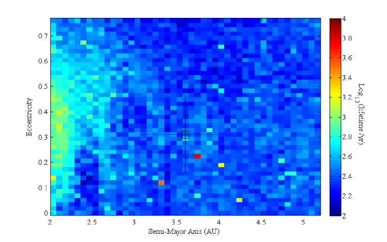
Figure 6: The stability of the HW Vir planetary system as proposed by Lee et al. (2009), as a function of the semi-major axis, $a$, and eccentricity, $e$, of planet HW Vir b. The initial orbit of HW Vir c was the same in each integration, set to the nominal best fit orbit from that work. The mean lifetime of the planetary system (in $log_{10}(lifetime/yr)$) at a given $a-e$ co-ordinate is denoted by the colour of the plot. The lifetime at each $a-e$ location is the mean value of 45 separate integrations carried of orbits at that $a-e$ position (testing a combination of 15 unique $\omega$ values, and 3 unique $M$ values). The nominal best-fit orbit for HW Vir b is located within the open square, from which lines radiate showing the extend of the $\pm~{}1$-$\sigma$ errors on $a$ and $e$. As can be seen, the orbits of the system are incredibly unstable, no matter what initial orbit is considered for HW Vir b.

In this way, the lifetime of each of the unique systems was determined. This, in turn, allowed us to construct a map of the dynamical stability of the system, which can be seen in Fig 6. As can be seen in that figure, none of the orbital solutions tested were dynamically stable, with few $a$-$e$ locations displaying mean lifetimes longer than 1,000 years.

Remarkably, we find that the proposed orbits for the HW Vir planetary system are even less dynamically stable than those proposed for the now discredited planetary system around HU Aqr (Horner et al., 2011; Wittenmyer et al., 2012a; Hinse et al., 2012a; Horner et al., 2012; Goździewski et al., 2012). Simply put, our result proves conclusively that, if there are planets in the HW Vir system, they must move on orbits dramatically different to those proposed by Lee et al. (2009). This instability is not particularly surprising, given the high orbital eccentricity of planet c, which essentially ensures that the two planets are on orbits that intersect one another, irrespective of the initial orbit of planet b. Given that the two planets are not trapped within mutual mean-motion resonance (MMR), such an orbital architecture essentially guarantees that they will experience strong close encounters within a very short period of time, ensuring the system’s instability.

4 Eclipse timing data analysis and LTT model

Given the extreme instability exhibited by the planets proposed by Lee et al. (2009), it seems reasonable to ask whether a re-analysis of the observational data will yield significantly different (and more reasonable) orbits for the planets in question. We therefore chose to re-analyse the observational data, following a similar methodology as applied in an earlier study of HU Aqr (Hinse et al., 2012a).

At the basis of our analysis we use the combined mid-eclipse timing data set compiled by Lee et al. (2009), including the times of secondary eclipses. The timing data used in Lee et al. (2009) were recorded in the UTC (Coordinated Universal Time) time standard, which is known to be non-uniform (Bastian, 2000; Guinan & Ribas, 2001). To eliminate timing variations introduced by accelerated motion within the Solar System, we therefore transformed the HJD (Heliocentric Julian Date) timing records in UTC time standard into Barycentric Julian Dates (BJD) within the Barycentric Dynamical Time (TDB) standard (Eastman et al., 2010). A total of 258 timing measurements were used spanning 24 years from January 1984 (HJD 2 445 730.6) to May 2008 (HJD 2 454 607.1). We assigned 1-$\sigma$ timing uncertainties to each data point by following the same approach as outlined in Lee et al. (2009).

For an idealised, unperturbed and isolated binary system, the linear ephemeris of future/past mid-eclipse (usually primary) events can be computed from

$$T_{C}(E)=T_{0}+P_{0}E,$$ (1)

where $E$ denotes the (independent) ephemeris cycle number, $T_{0}$ is the reference epoch, and $P_{0}$ measures the eclipsing period ($\simeq 2.8$ hrs) of HW Vir. A linear regression performed on the 258 recorded light-curves allows $P_{0}$ to be determined with high precision. In this work, we chose to place the reference epoch close to the middle of the observing baseline to avoid parameter correlation between $T_{0}$ and $P_{0}$ during the fitting process. In the following we briefly outline the LTT model as used in this work.

4.1 Analytic LTT model

The model adopted in this work is similar to that described in Hinse et al. (2012a), and is based on the original formulation of a single light-travel time orbit introduced by Irwin et al. (1952). In this model the two components of the binary system are assumed to represent one single object with a total mass equal to the sum of the masses of the two stars. This point mass is then placed at the original binary barycentre. If a circumbinary companion exist, then the combined binary mass follows an orbit around the total system barycentre. The eclipses are then given by Eq. 1. This defines the LTT orbit of the binary. The underlying reference system has its origin at the total centre of mass.

Following Irwin et al. (1952), if the observed mid-eclipse times exhibit a sinusoidal-like variation (due to one or more unseen companion(s)), then the quantity $O-C$ defines the light-travel time effect and is given by

$$(O-C)(E)=T_{O}(E)-T_{C}(E)=\sum_{i=1}^{2}\tau_{i},$$ (2)

where $T_{O}$ denotes the measured time of an observed mid-eclipse, and $T_{C}$ is the computed time of that mid-eclipse based on a linear ephemeris. We note that $\tau_{1}+\tau_{2}$ is the combined LTT effect from two separate two-body LTT orbits. The quantity $\tau_{i}$ is given by the following expression for each companion (Irwin et al., 1952):

$$\tau_{i}=K_{b,i}\Big{[}\frac{1-e_{b,i}^{2}}{1+e_{b,i}\cos f_{b,i}}\sin(f_{b,i}+\omega_{b,i})+e_{b,i}\sin\omega_{b,i}\Big{]},$$ (3)

where $K_{b,i}=a_{b,i}\sin I_{b,i}/c$ is the semi-amplitude of the light-time effect (in the $O-C$ diagram) with $c$ measuring the speed of light and $I_{b,i}$ is the line-of-sight inclination of the LTT orbit relative to the sky plane, $e_{b,i}$ the orbital eccentricity, $f_{b,i}$ the true longitude and $\omega_{b,i}$ the argument of pericenter of the LTT orbit. The 5 model parameters for a single LTT orbit are given by the set $(a_{b,i}\sin I_{b,i},e_{b,i},\omega_{b,i},T_{b,i},P_{b,i})$. The time of pericentre passage $T_{b,i}$ and orbital period $P_{b,i}$ are introduced through the expression of the true longitude as a time-like variable via the mean anomaly $M=n_{b,i}(T_{O}-T_{b,i})$, with $n_{b,i}=2\pi/P_{b,i}$ denoting the mean motion of the combined binary in its LTT orbit. Computing the true anomaly as a function of time (or cycle number) requires the solution of Kepler’s equation. We direct the interested reader to Hinse et al. (2012a) for further details.

In Eq. 3, the origin of the coordinate system is placed at the centre of the LTT orbit (see e.g. Irwin et al., 1952). A more natural choice (from a dynamical point of view) would be to use the system centre of mass as the origin of the coordinate system. However, the derived Keplerian elements are identical in the two coordinate systems (e.g. Hinse et al., 2012b). Finally, we note that our model does not include mutual gravitational interactions. We also only consider the combination of two LTT orbits from two circumbinary companions.

From first principles, some similarities exist between the LTT orbit and the orbit of the circumbinary companion. First, the eccentricities ($e_{b,i}=e_{i}$) and orbital periods ($P_{b,i}=P_{i}$) are the same. Second, the arguments of pericenter are $180^{\circ}$ apart from one another ($\omega_{i}=180^{\circ}-\omega_{b,i}$). Third, the times of pericenter passage are also identical ($T_{b,i}=T_{i}$).

Information of the mass of the unseen companion can be obtained from the mass function given by

$$f(m_{i})=\frac{4\pi^{2}(a_{b,i}\sin I_{b,i})^{3}}{GP_{b,i}^{2}}=\frac{4\pi^{2}(K_{b,i}c)^{3}}{GP_{b,i}^{2}}=\frac{(m_{i}\sin I_{i})^{3}}{(m_{b}+m_{i})},~{}~{}~{}~{}~{}i=1,2$$ (4)

The least-squares fitting process provides a measure for $K_{b,i}$ and $P_{b,i}$, and hence the minimum mass of the companion can be found from numerical iteration. In the non-inertial astrocentric reference frame, with the combined binary mass at rest, the companion’s semi-major axis relative to the binary is then calculated using Kepler’s third law.

In Lee et al. (2009) the authors also accounted for additional period variations due to mass transfer and/or magnetic interactions between the two binary components. These variations usually occur on longer time scales compared to orbital period variations due to unseen companions. Following Hilditch (2001), the corresponding ephemeris of calculated times of mid-eclipses then takes the form

$$T_{C}=T_{0}+P_{0}E+\beta E^{2}+\tau_{i},~{}~{}~{}~{}~{}i=1,2$$ (5)

where $\beta$ is an additional free model parameter and accounts for a secular modulation of the mid-eclipse times resulting from interactions between the binary components. Assuming the timing data of HW Vir are best described by a two-companion system, and to be consistent with Lee et al. (2009), we have used Eq. 5 as our model which consists of 13 parameters.

5 Methodology and results from $\chi^{2}$-parameter search

To find a stable orbital configuration of the two proposed circumbinary companions, we carried out an extensive search for a best-fit in $\chi^{2}$ parameter space. The analysis, methodology and technique follow the same approach as outlined in Hinse et al. (2012a). Here we briefly repeat the most important elements in our analysis.

We used the Levenberg-Marquardt least-square minimisation algorithm as implemented in the IDL-based software package MPFIT (Markwardt, 2009). The goodness-of-fit statistic $\chi^{2}$ of each fit was evaluated from the weighted sum of squared errors. In this work, we use the reduced chi-square statistic $\chi^{2}_{r}$ which takes into account the number of data points and the number of freely varying model parameters.

We seeded 28,201 initial guesses within a Monte Carlo experiment. Each guess was allowed a maximum of 500 iterations before termination, with all 13 model parameters (including the secular term) kept freely varying. Converged solutions with $\chi^{2}_{r}\leq 10$ were accepted with the initial guess and final fitting parameters recorded to a file. After each converged iteration we also solved the mass function (Eq. 4) for the companion’s minimum mass and calculated the semi-major axis relative to the system barycentre from Kepler’s third law.

Initial guesses of the model parameters were chosen at random following either a uniform or normal distribution. For example, initial orbital eccentricities were drawn from a uniform distribution within the interval $e\in[0.0,0.8]$. Our initial guesses for the orbital periods were guided by a Lomb-Scargle (LS) discrete Fourier transformation analysis on the complete timing data set. For the LS analysis we used the PERIOD04 software package (Lenz & Breger, 2005) capable of analysing unevenly sampled data sets. Fig. 1 shows the normalised LS power-spectrum. The LS algorithm found two significant periods with frequencies $f_{1}\simeq 1.4\times 10^{-4}~{}\textnormal{cycles/day}$ and $f_{2}\simeq 2.1\times 10^{-4}~{}\textnormal{cycles/day}$. These frequencies correspond to periods of 7397 and 4672 days, respectively. Hence the short-period variation is covered more than twice during the observing interval. Due to a lower amplitude, it contains less power within the data set. Our random initial guesses for the companion periods were then drawn from a Gaussian distribution centred at these periods with standard deviation of $\pm~{}5$ years. We call this approach a “quasi-global” search of the underlying $\chi^{2}$-parameter space.

5.1 Results - finding best fit and confidence levels

Our best fit model resulted in a $\chi^{2}_{r}=0.943$ and is shown in Fig. 2 along with the LTT signal due to the inner and outer companion and the secular term. The corresponding root-mean-square (RMS) scatter of data around the best fit is 8.7 seconds, which is close to the RMS scatter reported in Lee et al. (2009). The fitted model elements and derived quantities of our best fit are shown in Table 2. Compared to the system in Lee et al. (2009) we note that we now obtain a lower eccentricity for the inner companion and a larger eccentricity for the outer companion. Furthermore, our two-companion system has also slightly expanded, with larger semi-major axes (and therefore longer orbital periods) for both companions compared to Lee et al. (2009).

The next question to ask is how reliable or significant our best-fit solution is in a statistical sense. Assuming that the errors are normally distributed one can establish confidence levels for a multi-parameter fit (Bevington & Robinson, 1992). We therefore carried out detailed two-dimensional parameter scans covering a large range around the best-fit value in order to study the $\chi^{2}_{r}$-space topology in more detail. In particular, we explored relevant model parameter combinations including $T_{0},P_{0}$ and $\beta$.

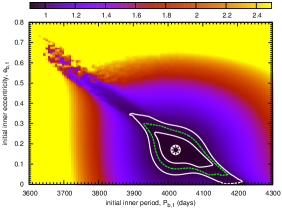
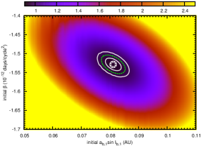
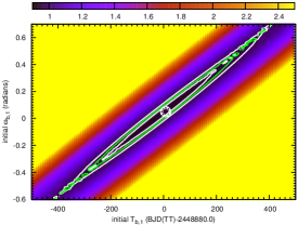
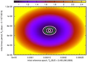
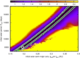
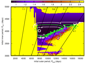
Figure 3: Colour-coded $\chi_{r}^{2}$ parameter scans of orbital parameters with remaining parameters to vary freely. The best-fit parameter is indicated by a star-like symbol. Contour curves show the 1,2,3$\sigma$ confidence level curves around our best-fit model. See electronic version for colour figures.

In all our experiments we allowed the remaining model parameters to vary freely while fixing the two parameters of interest in the considered parameter range (Bevington & Robinson, 1992; Press et al., 1992). Assuming parameter errors are normally distributed, our 1-, 2- and 3-$\sigma$ level curves provide the 68.3, 95.4 and 99.7% confidence levels relative to our best-fit, respectively. In Fig. 3 we show a selection of our two-dimensional parameter scan considering various model parameters.

Ideally, one would aim to work with parameters with little correlation between the two parameters. The lower-right panel in Fig. 3 shows the relationship between $T_{0}$ and $P_{0}$. The near circular shape of the level curves reveals that little correlation between the two parameters exists. This is most likely explained by our choice to locate the reference epoch in the middle of the dataset. The remaining panels in Fig. 3 show some correlations between the parameters. However, we have some indication of an unconstrained outer orbital period in the lower-left panel of Fig. 3. We show the location of orbital mean motion resonances in the $(P_{1},P_{2})$ plane. Our best fit is located close to the 2:1 mean motion resonance.

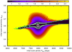
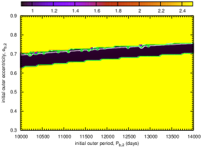
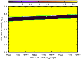
Figure 4: Same as Fig. 3 but considering the $(P_{2},e_{2})$-plane. The middle and right panel shows the $\chi^{2}_{r}$ topology for longer orbital periods of the outer companion. Based on the used data set, no firm confidence levels can be established around out best-fit value.

To demonstrate that the outer period is unconstrained we have generated $\chi^{2}_{r}$-parameter scans in the $(P_{2},e_{2})$-plane as shown in Fig. 4. Our best fit model is shown in the left-most panel of Fig. 4, along with the 1-,2- and 3-$\sigma$ confidence levels. It is readily evident that the 1-$\sigma$ confidence level does not simply surround our best-fit model in a confined or ellipsoidal manner. We rather observe that all three level curves are significantly stretched towards solutions featuring longer orbital periods for the outer companion. This is demonstrated in the middle and right panels of Fig. 4. Any longer orbital period for the outer companion therefore results in a $\chi^{2}_{r}$ with similar statistical significance as our best-fit model.

In addition, we studied the $(a\sin i,P)$-parameter plane for the outer companion, as shown in the lower-middle panel of Fig. 3. Here, we also observe that $a\sin i$ is unconstrained. The unconstrained nature of the outer companion’s $a\sin i$ and orbital period has a dramatic effect on the derived minimum mass and the corresponding error bounds.

5.2 Results - parameter errors

When applying the LM algorithm formal parameter errors are obtained from the best-fit covariance matrix. However, in our study, we sometimes encounter situations where some of the matrix elements become zero, or have singular values. However, at others times, the error matrix is returned with non-zero elements. In those cases we have observed that the outer orbital period is often better determined than that of the inner companion. In the case of HW Vir, such solutions are clearly incongruous, given the relatively poor orbital characterisation of the outer body compared to that of the innermost.

Being suspicious about the formal covariance errors, we have resorted to two other methods to determine parameter errors. First, we attempted to determine errors by the use of the bootstrap method (Press et al., 1992). However, we found that the resulting error ranges are comparable to the formal errors extracted from the best-fit covariance matrix. Furthermore, the bootstrap error ranges were clearly incompatible with the 1-$\sigma$ error “ellipses” discussed above. For example, from the top-left panel in Fig. 3 we estimate the 1-$\sigma$ error on the inner orbital period to be on the order of 50-100 days. In contrast, the errors for the inner orbital period obtained from our bootstrap method were of order just a few days. For this reason, we consider the bootstrap method to have failed, and it has therefore not been investigated further in this study. However, it is interesting to speculate on the possibility of dealing with a dataset which is characterised by “clumps of data”, as seen in Fig. 2. When generating random (with replacement) bootstrap ensembles, there is the possibility that only a small variation is being introduced for each random draw, as a result of the clumpiness of the underlying dataset. That clumpiness might be mitigated for, and the bootstrap method rendered still viable for the establishment of reliable errors, by enlarging the number of bootstrap ensembles to compensate for the lack of variation within single bootstrap data sets. One other possibility would be to replace clumps of data by a single data point reflecting the average of the clump. However, we have instead invoked a different approach.

Having located a best-fit minimum, we again seeded a large number of initial guesses around the best-fit parameters. This time, we considered only a relatively narrow range around the best-fit values (e.g. as shown in Fig. 3 and Fig. 4. This ensured that the LM algorithm would iterate towards our best-fit model depending on the underlying $\chi^{2}_{r}$ topology and inter-parameter correlations. The initial parameter guesses were randomly drawn from a uniform distribution within a given parameter interval. We then iterated towards a best-fit value using LM, and recorded the best-fit parameters along with the corresponding $\chi^{2}_{r}$.

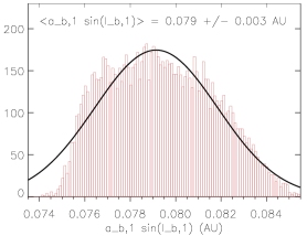
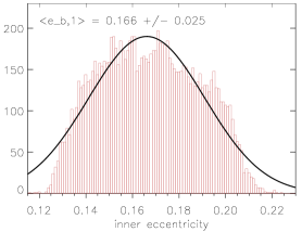
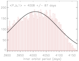
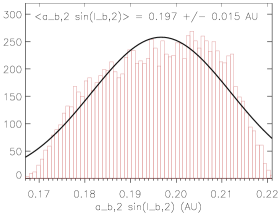
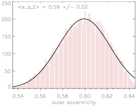
Figure 5: Histogram distribution of six model parameters as obtained from a Monte Carlo experiment. Only models with $\chi^{2}_{r}<1-\sigma$ where considered to assess the 68% confidence levels for each parameter. Solid curves show fitted normal distribution with mean and standard deviation indicated in each panel. However, we used the mean and standard deviation derived from the underlying dataset to derive our 1-$\sigma$ errors as quoted in Table 2.

Generating a large number of guesses enabled us to establish statistics on the final best-fit parameters with $\chi^{2}_{r}$ within 1-, 2-, and 3-$\sigma$ confidence levels. We therefore performed a Monte Carlo experiment that considered several tens of thousands of guesses. To establish 1-$\sigma$ error bounds (assuming a normal distribution for each parameter), we then considered only those models that yielded $\chi^{2}_{r}$ within the 1-$\sigma$ confidence limits (inner level curves), as shown in Fig. 3 and Fig. 4. The error for a given parameter is then obtained from the mean and standard deviation, and listed in Table 2. In order to test our assumption of normally distributed errors, we plotted histograms for the various model parameters in Fig. 5. For each histogram distribution, we fitted a Gaussian and established the corresponding mean and standard deviation. While some parameters follow a Gaussian distribution (for example the outer companion’s eccentricity), other parameters show no clear sign of “Gaussian tails”. This is especially true for the orbital period of the outer companion. Following two independent paths of analysis, we have demonstrated that the outer period is unconstrained, based on the present dataset, and should be regarded with some caution. However, we also point out a short-coming of our method of determining random parameter errors. The parameter estimates depend on the proximity of the starting parameters to the best-fit parameter. In principle, our method of error determination assumes that the best-fit model parameters are well-determined in terms of well-established closed-loop confidence levels around the best-fit parameters. The true random parameter error distribution for the two ill-constrained parameters might turn out differently. To put stronger constraints on the model parameters is clearly only possible by augmenting the existing timing data through a program of continuous monitoring of HW Vir over the coming years (Pribulla et al., 2012; Konacki et al., 2012). As more data is gathered, the confidence levels in Fig. 4 will eventually narrow down.

6 The $\beta$ coefficient and angular momentum loss

One of the features of our best-fit orbital solution is that it results in a relatively large $\beta$ coefficient, which can be related to a change in the period of the binary resulting from additional, non-planetary effects. Potential causes of such a period change include mass transfer, loss of angular momentum, magnetic interactions between the two binary components and/or perturbations from a third body on a distant and unconstrained orbit. In this study, the $\beta$ factor represents a constant binary period change (see Hilditch, 2001, p. 171) with a linear rate of $dP/dt=-9.57\times 10^{-9}~{}\textnormal{days/yr}$, which is about 15 percent larger than the value reported in Lee et al. (2009). We retained the $\beta$ coefficient in our model in order that our treatment be consistent with that detailed in Lee et al. (2009), such that our results might be directly compared to their work.

Lee et al. (2009) examined a number of combinations of models that incorporated a variety of potential causes for the observed period modulation. They found that the timing data is best described by two LTT and a quadratic term in the linear ephemeris model. In their work, Lee et al. (2009) carefully examined the contribution of period modulation by various astrophysical effects. They were able to provide arguments that rule out the operation of the Applegate mechanism, due to the lack of small-scale variations in the observed luminosities that would have an influence on the $J_{2}$ oblateness coefficient of the magnetically active component. A change in $J_{2}$ would, in turn, affect the binary period.

Furthermore, Lee et al. (2009) reject the idea that the observed $O-C$ variation could be the result of apsidal motion, based on the circular orbit of the HW Vir binary system. In addition, they estimated the secular period change of the HW Vir binary orbit due to angular momentum loss through gravitational radiation and magnetic breaking. They found that the most likely explanation for the observed linear decrease in the binary period is that it is the result of angular momentum loss by magnetic stellar wind breaking in the secondary M-type component. From first principles (e.g. Brinkworth et al., 2006), the period change observed in this work corresponds to a angular momentum change of order $dJ/dt=-2.65\times 10^{36}$ erg. This is approximately 15 percent larger than the value reported by Lee et al. (2009), but still well within the range where magnetic breaking is a reasonable astrophysical cause for period modulation.

Finally, we note that, whilst this work was under review, Beuermann et al. (2012) published a similar study based on new timing data, in which they also considered the influence of period changes due to additional companions. In their work, they obtained a markedly different orbital solution than those discussed in this work, one which they found to be dynamically stable on relatively long timescales. In light of their findings, it is interesting to note that they do not include a quadratic term in their linear ephemeris model. This could point at the possibility that the inclusion of a quadratic term is somehow linked to the instability of the best-fit system found in this work.

Beuermann et al. (2012) found stable orbits for a solution involving two circumbinary companions. However, despite this, we note that the two models share some qualitative characteristics. A careful examination of Fig. 2 in Beuermann et al. (2012) reveals that the orbital period of the outer companion is unconstrained from a period analysis since the $\chi^{2}$-contour curves are open towards longer outer orbital periods - a result mirrored in our current work. As we noted earlier, we were unable to place strict confidence levels on the best-fit outer companion’s orbital period and semi-major axis. Although Beuermann et al. (2012) do find a range of stable scenarios featuring their outer companion, we note that they fixed the eccentricity of that companion’s orbit to be near-circular, with period of 55 years. Such an assumption (i.e. fixing some orbital parameters) is somewhat dangerous, since it can lead to the production of dynamically stable solutions that are not necessarily supported by the observational data (e.g. Horner et al., 2012). A more rigorous strategy would be to generate an ensemble of models with each model (all parameters freely varying) tested for orbital stability (using some criterion like non-crossing orbits or non-overlap of mean-motion resonances, etc.) resulting in a distribution of stable best-fit models. Using the new data set, a study of the distribution of the best-fit outer planet’s eccentricity would be interesting. It is certainly possible that the new data set constrains this parameter sufficiently in order to validate their assumptions. Although the results presented in Beuermann et al. (2012) are clearly promising, it is definitely the case that more observations are needed before the true origin of the observed variation for HW Vir is established beyond doubt.

The question of whether a period damping factor is truly necessary for the HW Vir system would require a statistically self-consistent re-examination of the complete data set taking account of a range of model scenarios. We refer the interested reader to Goździewski et al. (2012), who recently carried out a detailed investigation of the influence of the quadratic term for various scenarios in their attempt to explain the timing data of the HU Aqr system.

7 Dynamical analysis of the best-fit LTT model

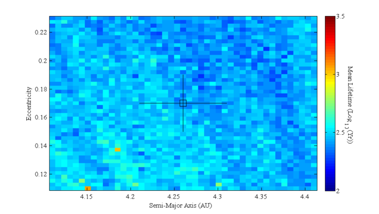
Figure 7: The stability of the HW Vir planetary system, given the orbital solution derived in this work, as a function of the semi-major axis, $a$, and eccentricity, $e$, of planet HW Vir b. The initial orbit of HW Vir c was the same in each integration, set to the nominal best fit orbit as detailed in Table 2. The mean lifetime of the planetary system (shown as $log_{10}(lifetime/yr$) at a given $a-e$ co-ordinate is denoted by the colour of the plot. The lifetime at each $a-e$ location is the mean value of 45 separate integrations carried of orbits at that $a-e$ position (testing a combination of 15 unique $\omega$ values, and 3 unique $M$ values). The nominal best-fit orbit for HW Vir b is located within the open square, from which lines radiate showing the extend of the $\pm~{}1$-$\sigma$ errors on $a$ and $e$. Once again, the orbits of the system are found to be incredibly unstable, no matter what initial orbit is considered for HW Vir b. The two red hotspots in that plot are the result of two unusually stable runs, with lifetimes of 33 kyr ($a=4.185$ AU, $e=0.137$) and 38 kyr ($a=4.15$ AU, $e=0.11$). Even these most extreme outliers are dynamically unstable on astronomically short timescales.

Since a detailed re-analysis of the observational data on the HW Vir system yields a new orbital solution for the system, it is interesting to consider whether that new solution offers better prospects for dynamical stability than that proposed in Lee et al. (2009). We therefore repeated our earlier dynamical analysis using the new orbital solution. Once again, we held the initial orbit of planet HW Vir c fixed at the nominal best-fit solution, and ran an equivalent grid of unique dynamical simulations of the planetary system, varying the initial orbit of HW Vir b such that a total of 45 distinct values of $a$ and $e$, 15 distinct values of $\omega$ and 3 values of $M$ were tested, each distributed evenly as before across the $\pm~{}3$-$\sigma$ range of allowed values. As before, the two simulated planets were assigned the nominal $M~{}\sin~{}i$ masses obtained from the orbital model. The results of our simulations can be seen in Fig. 7.

As was the case for the original orbital solution proposed in Lee et al. (2009), and despite the significantly reduced uncertainties in the orbital elements for the resulting planets, very few of the tested planetary systems survived for more than 1,000 years (with just twenty six systems, 0.029% of the sample, surviving for more than 3,000 years, and just three systems surviving for more than 10,000 years). As was the case for the planetary system proposed to orbit the cataclysmic variable system HU Aqr (e.g. Horner et al., 2011; Wittenmyer et al., 2012a), it seems almost certain that the proposed planets in the HW Vir system simply do not exist - at least on orbits resembling those that can be derived from the observational data.

8 Conclusion and Discussion

The presence of two planets orbiting the evolved binary star system HW Vir was proposed by Lee et al. (2009), on the basis of periodic variations in the timing of eclipses between the two stars. The planets proposed in that work were required to move on relatively eccentric orbits in order to explain the observed eclipse timing variations, to such a degree that the orbit of the outer planet must cross that of the innermost. It is obvious that, when one object moves on an orbit that crosses that of another, the two will eventually encounter one another, unless they are protected from such close encounters by the influence of a mutual mean-motion resonance (e.g. Horner et al., 2004a, b). Even objects protected by the influence of such resonances can be dynamically unstable, albeit on typically longer timescales (e.g. Horner & Lykawka, 2010; Horner, Müller & Lykawka, 2012; Horner et al., 2012). Since the two planets proposed by Lee et al. (2009) move on calculated orbits that allow the them to experience close encounters and yet are definitely not protected from such encounters by the influence of mutual mean-motion resonance, it is clear that they are likely to be highly dynamically unstable. To test this hypothesis, we performed a suite of highly detailed dynamical simulations of the proposed planetary system to examine its dynamical stability as a function of the orbits of the proposed planets. We found the proposed system to be dynamically unstable on extremely short timescales, as was expected based on the proposed architecture for the system.

Following our earlier work (Wittenmyer et al., 2012a; Hinse et al., 2012a), we performed a highly detailed re-analysis of the observed data, in order to check whether such improved analysis would yield better constrained orbits that might offer better prospects for dynamical stability. Our analysis resulted in calculated orbits for the candidate planets in the HW Vir system that have relatively small uncertainties. Once these orbits had been obtained, we performed a second suite of detailed dynamical simulations to ascertain the dynamical stability of the newly determined orbits. Following the same procedure as for the original orbits, we considered the stability of all plausible architectures for the HW Vir system. Despite the increased precision of the newly determined orbits, we find that the planetary system proposed is dynamically unstable on timescales as short as a human lifetime. For that reason, we must conclude that the eclipse-timing variations observed in the HW Vir system are not solely down to the gravitational influence of perturbing planets. Furthermore, if any planets do exist in that system, they must move on orbits dramatically different to those considered in this work.

Our results highlight the importance of performing complementary dynamical studies of any suspected multiple-exoplanet system – particularly in those cases where the derived planetary orbits approach one another closely, are mutually crossing and/or derived companion masses are large. Following a similar strategy as applied to the proposed planetary system orbiting HU Aqr (Horner et al., 2011; Wittenmyer et al., 2012a; Goździewski et al., 2012), we have found that the proposed 2-planet system around HW Vir does not stand up to a detailed dynamical scrutiny. In this work we have shown that the outer companion’s period (among other parameters) is heavily unconstrained by establishing confidence limits around our best-fit model. However, we also point out the fact that the two circumbinary companions have brown-dwarf masses. Hence, a more detailed $n$-body LTT model which takes account of mutual gravitational interactions might provide a better description of the problem.

To further characterise the HW Vir system and constrain orbital parameters we recommend further observations within a monitoring program as described in Pribulla et al. (2012). In a recent work on HU Aqr, Goździewski et al. (2012) pointed out the possibility that different data sets obtained from different telescopes could introduce systematic errors resulting in a false-positive detection of a two-planet circumbinary system.

Finally, we note that, whilst this paper was under referee, Beuermann et al. (2012) independently published their own new study of the HW Vir system. Based on new observational timing data, those authors determined a new LTT model that appears to place the 2-planet system around HW Vir on orbits that display long-term dynamical stability. Based on the results presented in this work, we somewhat doubt their findings of a stable 2-planet system and question whether such a system is really supported by the new data set given that no strict confidence levels were found for the best-fit outer period. Since performing a full re-analysis of their newly compiled data, including dynamical mapping of their new architecture, would be a particularly time intensive process, we have chosen to postpone this task for a future study.

Figure 1: Power spectrum of HW Vir timing data set using BJD(TDB) times with the $O-C$ residuals measured in seconds. Two periods were found with $1/f_{1}=7397$ and $1/f_{2}=4672$ days, corresponding to 20.3 and 12.8 years, respectively. S/N denotes the frequency signal-to-noise ratio, which are significantly larger than the spectrum’s noise level. Normalisation was done by division of the maximum amplitude in each spectrum. The $f_{2}$-frequency was determined from the residuals after subtracting the period $1/f_{1}$ from the original timing data set. Additional peaks in both panels represent 1-year alias frequencies due to the repeating annual observing cycle of HW Vir.

Figure 2: Best-fit two-Kepler LTT model with $\chi_{r}^{2}=0.943$. The best-fit model parameters (including reference epoch) are shown in Table 2.RMS denotes the root-mean-square scatter around the best fit. The lower part of the figure shows the residuals between the best fit model and the observed timing data set.

Parameter		two-LTT		Unit
		$\tau_{1}~{}(i=1)$	$\tau_{2}~{}(i=2)$
$\chi_{r}^{2}$		0.943		-
RMS		8.665		seconds
$\beta$		$-1.529\cdot 10^{-12}\pm 1.25\cdot 10^{-13}$		$\textnormal{day/cycle}^{2}$
$T_{0}$		$2,450,280.28596\pm 2.3\cdot 10^{-5}$		BJD(TDB)
$P_{0}$		$0.116719519\pm 4.6\cdot 10^{-9}$		days
$a_{b,i}\sin I_{b,i}$		$0.081\pm 0.002$	$0.196\pm 0.012$	AU
$e_{b,i}~{}~{}(\textnormal{or}~{}e_{1,2})$		$0.17\pm 0.02$	$0.61\pm 0.02$	-
$\omega_{b,i}$		$0.05\pm 0.01$	$2.09\pm 0.08$	rad.
$T_{b,i}$		$2,448,880\pm 57$	$2,448,629\pm 42$	BJD(TT)
$P_{b,i}~{}~{}(\textnormal{or}~{}P_{1,2})$		$4021\pm 64$	$7992\pm 551$ (!)	days
$K_{b,i}$		$4.6\cdot 10^{-4}\pm 1.3\cdot 10^{-5}$	$1.13\cdot 10^{-3}\pm 7.04\cdot 10^{-5}$	days
$m_{i}\sin I_{i}$		$12\pm 3$	$11\pm 8$	$M_{Jup}$
$a_{i}\sin I_{i}$		$4.26\pm 0.05$	$6.8\pm 0.3$	AU
$e_{i}$		$0.17\pm 0.02$	$0.61\pm 0.02$	-
$\omega_{i}$		$(\pi-0.05)\pm 0.01$	$(\pi-2.09)\pm 0.08$	rad.
$T_{i}$		$2,448,880\pm 57$	$2,448,629\pm 42$	BJD(TT)
$P_{i}$		$4021\pm 64$	$7992\pm 551$ (!)	days

Table 2: Best-fit parameters for the LTT orbits of HW Vir corresponding to Fig. 2. Subscripts $1,2$ refer to the circumbinary companions with $i=1$, the inner, and $i=2$, the outer, companions. RMS measures the root-mean-square scatter of the data around the best fit. 1-$\sigma$ uncertainties have been obtained as described in the text. The last five entries are quantities of the two companions in the astrocentric coordinate system. Note that our values for $a$ and $P$ are somewhat larger than those of Lee et al. (2009): $a_{b}=3.62$ and $a_{c}=5.30$ AU, $P_{b}=3316$ and $P_{c}=5786$ days.

References

- Anglada-Escudé et al. (2012) Anglada-Escudé, G., Arriagada, P., Vogt, S. S., et al. 2012, arXiv:1202.0446
- Applegate (1992) Applegate, J. H. 1992, ApJ, 385, 621
- Bakos et al. (2007) Bakos, G. Á., Noyes, R. W., Kovács, G., et al. 2007, ApJ, 656, 552
- Barlow et al. (2011) Barlow, B. N., Dunlap, B. H., Clemens, J. C., 2011 ApJ, 737, 2
- Bastian (2000) Bastian, U. 2000, IBVS, 4822
- Beuermann et al. (2010) Beuermann K., et al. 2010, A&A, 521, L60
- Beuermann et al. (2012) Beuermann K., et al. 2012, A&A, in press, 2012arXiv1206.3080B
- Bevington & Robinson (1992) Bevington, P. R., & Robinson, K. D., McGraw-Hill, 2nd ed., 1992
- Borucki et al. (2011) Borucki, W. J., Koch, D. G., Basri, G., et al. 2011, ApJ, 728, 117
- Brinkworth et al. (2006) Brinkworth, C. S., Marsh, T. R., Dhillon, V. S., Knigge, C., 2006, MNRAS, 365, 287
- Chambers & Migliorini (1997) Chambers, J. E., Migliorini, F. 1997, BAAS, 27-06-P
- Chambers (1999) Chambers, J. E. 1999, MNRAS, 304, 793
- Doyle et al. (2011) Doyle, L. R., Carter, J. A., Fabrycky, D. C., et al. 2011, Science, 333, 1602
- Eastman et al. (2010) Eastman, J., Siverd, R., Gaudi, B. S. 2010, PASP, 122, 935
- Endl et al. (2006) Endl, M., Cochran, W. D., Wittenmyer, R. A., & Hatzes, A. P. 2006, AJ, 131, 3131
- Ferraz-Mello et al. (2005) Ferraz-Mello, S., Michtchenko, T. A., & Beaugé, C. 2005, ApJ, 621, 473
- Funk et al. (2011) Funk, B., et al. 2011, (submitted to MNRAS)
- Funk et al. (2011) Funk, B., Eggl, S., Gyergyovits, M., Schwarz, R., & Pilat-Lohinger, E. 2011, EPSC-DPS Joint Meeting 2011, 1725
- Goździewski & Maciejewski (2001) Goździewski, K., & Maciejewski, A. J. 2001, ApJL, 563, L81
- Goździewski, Konacki & Maciejewski (2003) Goździewski, K., Konacki, M., Maciejewski, A. J., 2003, ApJ, 594, 1019
- Goździewski et al. (2012) Goździewski, K., Nasiroglu, I., Slowikowska, A., et al. 2012, MNRAS, in press, (eprint arXiv:1205.4164)
- Goździewski, Konacki & Maciejewski (2005) Goździewski, K., Konacki, M., Maciejewski, A. J., 2005, ApJ, 622, 1136
- Guinan & Ribas (2001) Guinan, E. F., Ribas, I., 2001, ApJL, 546, L43
- Hellier et al. (2011) Hellier, C., Anderson, D. R., Collier Cameron, A., et al. 2011, A&A, 535, L7
- Hilditch (2001) Hilditch, R. W., “An introduction to close binary stars”, 2001, 1st ed., Cambridge University Press
- Hinse et al. (2012a) Hinse, T. C., Lee, J. W., Goździewski, K., Haghighipour, N., Lee, C.-U., Scullion, E. M., 2012, MNRAS, 420, 3609
- Hinse et al. (2012b) Hinse, T. C., Goździewski, K., Lee, J. W., Haghighipour, N., Lee, C.-U., 2012, AJ, 144, 34
- Horner et al. (2004a) Horner, J., Evans, N. W., & Bailey, M. E. 2004, MNRAS, 354, 798
- Horner et al. (2004b) Horner, J., Evans, N. W., & Bailey, M. E. 2004, MNRAS, 355, 321
- Horner & Lykawka (2010) Horner, J., & Lykawka, P. S. 2010, MNRAS, 405, 49
- Horner, Müller & Lykawka (2012) Horner, J., Müller, T. G. & Lykawka, P. S., 2012, MNRAS, 423, 2587
- Horner et al. (2012) Horner, J., Lykawka, P. S., Bannister, M. T., & Francis, P., 2012, MNRAS, 422, 2145
- Horner et al. (2011) Horner, J., Marshall, J., Wittenmyer, R., Tinney, Ch. 2011, MNRAS, 416, L11
- Horner et al. (2012) Horner, J., Wittenmyer, R. A., Hinse, T. C., & Tinney, C. G. 2012, MNRAS, in press
- Howard et al. (2010) Howard, A. W., Johnson, J. A., Marcy, G. W., et al. 2010, ApJ, 721, 1467
- Howard et al. (2012) Howard, A. W., Bakos, G. Á., Hartman, J., et al. 2012, ApJ, 749, 134
- İbanoǧlu et al. (2004) İbanoǧlu, C., Çakırlı, Ö., Taş, G., & Evren, S. 2004, A&A, 414, 1043
- Irwin et al. (1952) Irwin, J. B., 1952, ApJ, 116, 211
- Irwin et al. (1959) Irwin, J. B., 1959, AJ, 64, 149
- Kilkenny et al. (1994) Kilkenny, D., Marang, F., & Menzies, J. W. 1994, MNRAS, 267, 535
- Kilkenny et al. (2003) Kilkenny, D., van Wyk, F., & Marang, F. 2003, The Observatory, 123, 31
- Konacki et al. (2012) Konacki, M., Sybilski, P., Kozłowski, S. K., Ratajczak, M., & Hełminiak, K. G. 2012, IAU Symposium, 282, 111
- Laskar & Correia (2009) Laskar, J., & Correia, A. C. M. 2009, A&A, 496, L5
- Lee et al. (2009) Lee J., et al., 2009, AJ, 137, 3181
- Lee et al. (2012) Lee J., et al., 2012, AJ, 143, 34
- Lenz & Breger (2005) Lenz P., Breger M. 2005, CoAst, 146, 53
- Malmberg & Davies (2009) Malmberg, D., Davies, M. B., 2009, MNRAS, 394, 26
- Markwardt (2009) Markwardt, C. B., 2009, ASPCS, “Non-linear Least-squares Fitting in IDL with MPFIT”, Astronomical Data Analysis Software and Systems XVIII, eds. Bohlender, D. A., Durand, D., Dowler, P.
- Marshall et al. (2010) Marshall, J., Horner, J., & Carter, A. 2010, International Journal of Astrobiology, 9, 259
- Mayor & Queloz (1995) Mayor, M., Queloz, D., 1995, Nature, 378, 355
- Mayor et al. (2009) Mayor, M., Udry, S., Lovis, C., et al. 2009, A&A, 493, 639
- Menzies & Marang (1986) Menzies, J. W., & Marang, F. 1986, Instrumentation and Research Programmes for Small Telescopes, 118, 305
- Murray & Dermott (2001) Murray, C. D., Dermott, S. F., 2001, Solar System Dynamics, Cambridge University Press.
- Pepe et al. (2004) Pepe, F., Mayor, M., Queloz, D., et al. 2004, A&A, 423, 385
- Potter et al. (2011) Potter, S. B., Romero-Colmenero, E., Ramsay, G., Crawford, S., Gulbis, A., Barway, S., Zietsman, E., Kotze, M., Buckley, D. A. H., O’Donoghue, D., Siegmund, O. H. W., McPhate, J., Welsh, B. Y., Vallerga, J., MNRAS, 416, 2202
- Press et al. (1992) Press, W. H., Saul, A. T., Vetterling, W. T., Flannery, B. P., Cambridge University Press, 2nd edition, 1992.
- Pribulla et al. (2012) Pribulla, T., Vaňko, M., Ammler- von Eiff, M., Andreev, M. et al. 2012, AN (submitted), eprint arXiv:1206.6709
- Rivera et al. (2010) Rivera, E. J., Laughlin, G., Butler, R. P., et al. 2010, ApJ, 719, 890
- Robertson et al. (2012a) Robertson, P., Endl, M., Cochran, W. D., et al. 2012a, ApJ, 749, 39
- Robertson et al. (2012b) Robertson, P., Horner, J., Wittenmyer, R. A. et al. 2012b, ApJ, 754, 50.
- Schwarz et al. (2009) Schwarz, R., Schwope, A. D., Vogel, J., Dhillon, V. S., Marsh, T. R., Copperwheat, C., Littlefair, S. P., Kanbach, G., 2009, A&A, 496, 833
- Schwope et al. (2001) Schwope, A. D., Schwarz, R., Sirk, M., Howell, S. B., 2001, A&A, 375, 419
- Schwope et al. (2011) Schwope, A. D.,Horne, K., Steeghs, D., Still, M., A&A, 531, 34
- Smith et al. (2012) Smith, A. M. S., Anderson, D. R., Collier Cameron, A., et al. 2012, A. J., 143, 81
- Stepinski et al. (2000) Stepinski, T. F., Malhotra, R., & Black, D. C. 2000, ApJ, 545, 1044
- Tinney et al. (2001) Tinney, C. G., Butler, R. P., Marcy, G. W., et al. 2001, ApJ, 551, 507
- Tinney et al. (2011) Tinney, C. G., Wittenmyer, R. A., Butler, R. P., et al. 2011, ApJ, 732, 31
- Qian et al. (2011) Qian, S.-B., et al., 2011, MNRAS, 414, L16
- Qian et al. (2010) Qian, S.-B., Liao, W.-P., Zhu, L.-Y., & Dai, Z.-B. 2010, ApJL, 708, L66
- Udry et al. (2007) Udry, S., Bonfils, X., Delfosse, X., et al. 2007, A&A, 469, L43
- Welsh et al. (2012) Welsh, W. F., Orosz, J. A., Carter, J. A., et al. 2012, Nature, 481, 475
- Wittenmyer et al. (2012a) Wittenmyer, R. A., Horner, J., Marshall, J. P., Butters, O. W., & Tinney, C. G. 2012a, MNRAS, 419, 3258
- Wittenmyer et al. (2012b) Wittenmyer, R. A., et al., 2012b, ApJ, in press
- Wolszczan & Frail (1992) Wolszczan, A., Frail, D. A., 1992, Nature, 355, 145
- Wood & Saffer (1999) Wood, J. H., & Saffer, R. 1999, MNRAS, 305, 820
- Wright et al. (2011) Wright, J. T., Veras, D., Ford, E. B., et al. 2011, ApJ, 730, 93