Quasiparticles and $Z(N)-$ lines in Hot Yang-Mills theories

Abstract

In this talk we review, the quasiparticle description of the hot Yang-Mills theories, in which the quasiparticles propagate in (and interact with) a background field related to $Z(N)$-lines. We compare the present description with a more common one in which the effects of the $Z(N)$-lines are neglected. We show that it is possible to take into account the nonperturbative effects at the confinement transition temperature even without a divergent quasiparticle mass.

1 Introduction

In recent years, the interest in understanding the thermodynamical properties of strong nonabelian mediums has noticeably increased. Lattice simulations of $SU(3)$ Yang-Mills theories Datta:2010sq ; Boyd:1996bx ; Boyd:1995zg ; Borsanyi:2011zm ; Borsanyi:2012ve agree about the onset of the deconfinenemt phase transition at $T=T_{c}\approx 270$ MeV. Below $T_{c}$, lattice data suggest the thermodynamics of the Yang-Mills theory is dominated by the lowest lying glueballs superimposed to a Hagedorn spectrum Borsanyi:2012ve . For what concerns the high temperature phase, the picture is not so clear. As a matter of fact, the perturbative regime is realized for very large temperatures, signalling the nonperturbative nature of the gluon medium above the critical temperature zwanziger2 . This makes the identification of the correct degrees of freedom of the gluon plasma, in proximity as well as well beyond the critical temperature, a very complicated task.

Beside resummation schemes based on the Hard Thermal Loop (HTL) approach HTL1 ; HTL3 ; HTL4 ; HTL7 ; Andersen_HTLpt ; Andersen:2010ct ; Andersen:2009tc and on the effective potential approach Braun:2007bx , the quasiparticle approach to the thermodynamics of QCD has attracted a discreet interest recently, see for example Refs. Gorenstein:1995vm ; PKPS96 ; Levai:1997yx ; bluhm-qpm ; Meisinger:2003id ; Castorina:2011ra ; Giacosa:2010vz ; Peshier:2005pp ; redlich ; Plumari:2011mk ; Filinov:2012pt ; Castorina:2007qv ; Castorina:2011ja ; Brau:2009mp ; Cao:2012qa ; Bannur:2006hp ; Sasaki:2012bi ; Ruggieri:2012ny and references therein. In such an approach, one identifies the degrees of freedom of the deconfinement phase with transverse gluons; the strong interaction in such a nonperturbative regime is taken into account through an effective temperature-dependent mass for the gluons themselves. Generally speaking, it is not possible to compute the self-energy of gluons exactly in the range of temperature of interest; as an obvious consequence, the location of the poles of the propagator in the complex momentum plane, hence (roughly speaking) the gluon mass, is an unknown function. For this reason, one usually assumes an analytic dependence of the gluon mass on the temperature, leaving few free parameters which are then fixed by fitting the thermodynamical data of Lattice simulations.

The advantage of such an approach is, at least, twofolds. Firstly, it is of a theoretical interest in itself to understand which are the effective degrees of freedom of the Yang-Mills theory at finite temperature and in particular the evolution of non perturbative effects with temperature. Furthermore, once a microscopic description of the plasma is identified, it is also possible to include the implied dynamics into a transport theory capable of directly simulating the expanding fireball produced in heavy ion collisions computing the collective properties, as well as the chemical composition of the fireball as a function of time Scardina:2012hy .

In this talk, we discuss the quasiparticle picture of the finite temperature gluon medium, by adding the interaction of gluons with a background Polyakov loop, or more generally speaking, with a background of traced $Z(N)-$lines according to the nomenclature given in Pisarski:2006hz . Within our picture, the common view of the deconfinement phase of $SU(3)$ theory as a gluon plasma, in which gluons are the relevant degrees of freedom, is replaced by a new one in which gluons propagate in a background of Polyakov loops, the latter being important degrees of freedom as much as the gluons are, since they embed nonperturbative informations about the deconfinement phase transition Polyakov:1978vu ; Susskind:1979up ; Svetitsky:1982gs ; Svetitsky:1985ye . This should be compared with the standard quasiparticle (plasma-like) picture, in which all the dynamics is taken into account by means of temperature dependent masses PKPS96 ; Levai:1997yx ; bluhm-qpm ; redlich ; Castorina:2011ra ; Castorina:2011ja ; Plumari:2011mk , leading to diverging or steadily increasing masses as $T\rightarrow T_{c}$. We show that combining a $T$-dependent quasiparticle mass, $M(T)$, with the Polyakov loop dynamics results in a quite different behavior of $M(T)$ as $T\rightarrow T_{c}$.

2 The model

The system we consider Ruggieri:2012ny consists of a gas of gluon quasiparticles, propagating in a background of Polyakov loops. For our purposes, considering fundamental and adjoint loops is enough. The free energy of the model is expressed as a linear combination of two contributions: the first one describes the thermodynamics of the Polyakov loop; the second one, on the other hand, is the contribution of gluon quasiparticles coupled to the Polyakov loop. We specify the two terms of the effective potential below.

For what concerns the Polyakov loop effective potential, following Abuki:2009dt ; Zhang:2010kn we consider the action of a pure matrix model Gupta:2007ax ,

$$S_{PM}[L]=-N_{c}^{2}e^{-a/T}\bm{\sum}_{\bm{x},\bm{y}}\ell_{F}(\bm{x})\ell_{F}^{*}(\bm{x}+\bm{y})~{},$$ (1)

where $\bm{x},\bm{y}$ denote the lattice site and its nearest neighbors respectively. Moreover $\ell_{F}(\bm{x})=\text{Tr}L_{F}(\bm{x})/N_{c}$ corresponds to the traced Polyakov loop in the fundamental representation. The Polyakov line in the representation ${\cal R}$ of the gauge group is given by

$$L_{\cal R}(\bm{x})={\cal P}\exp\left[i\int_{0}^{1/T}d\tau~{}A_{4}^{a}(\bm{x},\tau)T_{a,{\cal R}}\right]~{},$$ (2)

where $T_{a,{\cal R}}$ are the gauge group generators in the representation ${\cal R}$, and $A_{4}^{a}$ corresponds to a background euclidean gluon field.

The model specified by Eq. (1) corresponds to a matrix model, the untraced Polyakov loops $L(\bm{x})$ corresponding to the dynamical degrees of freedom. In this study we limit ourselves to the one-loop approximation; at this level, the effective potential for the Polyakov loop reads Ruggieri:2012ny

$$\Omega_{PM} = bT\left(-6N_{c}^{2}e^{-a/T}\langle\ell_{F}\rangle^{2}+N_{c}\left[\alpha\langle\ell_{F}\rangle\right]-\log\int dL~{}e^{N_{c}\left[\alpha\Re\ell_{F}\right]}\right)~{}.$$ (3)

Here $\alpha$ corresponds to a variational parameter, whose value at a given temperature is determined by the condition $\partial\Omega/\partial\alpha=0$; the average $\langle\ell_{F}\rangle$ is a function of $\alpha$, which we compute numerically. Besides, $a$ and $b$ in the above equation are treated as free parameters, whose value will be specified below.

The transverse gluon quasiparticle contribution to the thermodynamic potential reads Meisinger:2003id ; Sasaki:2012bi ; Ruggieri:2012ny

$$\Omega_{qp}=2T\int\frac{d^{3}k}{(2\pi)^{3}}\text{Tr}_{A}\log\left(1-L_{A}~{}e^{-E(k)/T}\right)~{}.$$ (4)

In the above equation, $L_{A}$ corresponds to the Polyakov line in the adjoint representation, as defined in Eq. (2), and the trace is taken over the indices of the adjoint representation of the gauge group. Moreover, the quasiparticle energy is given by $E(k)=\sqrt{k^{2}+M^{2}}$, where $M$ is supposed to arise from non-perturbative medium effects. In the case of very high temperature, where the gauge theory is in the perturbative regime and thus $M=0$, it can be proved that Eq. (4) is the effective potential for the adjoint Polyakov loop Weiss:1980rj . At lower temperatures, where non-perturbative effects are important, Eq. (4) must be postulated as a starting point for a phenomenological description of the thermodynamics of the gluon plasma. In this article, we make use of a temperature depentent mass whose analytic form is given by Peshier:2005pp ; Ruggieri:2012ny

$$M^{2}=\frac{8\pi^{2}T^{2}}{11\log\left[\lambda(T-w)\right]^{2}}~{}.$$ (5)

The parameters $w,\lambda$ are determined by requiring that, for pressure and energy density, the mean quadratic deviation between our theoretical computation and the Lattice data of Boyd:1996bx is a minimum.

In order to have a combined description of the gluon plasma around the critical temperature, in terms of the Polyakov loop (which acts as a background field) and of gluons quasiparticles (which propagate in the Polyakov loop background), we add Eq. (4) to the strong coupling inspired potential in Eq. (3). In order to do this, and to be consistent at the same time with the Weiss mean field procedure outlined above, we follow the lines of Abuki:2009dt and write the thermodynamic potential as

$$\Omega=\Omega_{PM}+\langle\Omega_{qp}\rangle~{},$$ (6)

where the averaged $\Omega_{qp}$ has to be understood as

$$\langle\Omega_{qp}\rangle=2T\int\frac{d^{3}k}{(2\pi)^{3}}~{}\log\left\langle\text{det}_{A}\left(1-L_{A}~{}e^{-E/T}\right)\right\rangle~{}.$$ (7)

We have checked numerically that in the deconfinement phase, at very large temperature $\langle\ell_{A}\rangle\approx 1$; as a consequence, the thermal distribution of the quasigluons approaches that of a perfect gas of massive particles in this limit. However, the thermodynamics of the system in the full range of temperature considered here remains different from the one of a mere massive gas because of the Polyakov background mean field.

3 Results

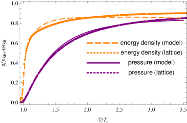
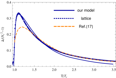
Figure 1: Left panel. Pressure (indigo, solid line) and energy density (orange, dashed line), normalized to the respective Stefan-Boltzmann values, as a function of temperature (measured in units of the critical temperature $T_{c}=270$ MeV), for the SU(3) case. Dots correspond to lattice data taken from Ref. Boyd:1996bx ; solid lines are the result of our numerical computation within the quasiparticle model. Right panel. Interaction measure per degree of freedom as a function of temperature. The dashed orange line corresponds to the result of Ref. Meisinger:2003id . Figure adapted from Ref. Ruggieri:2012ny .

In this talk, we focus on our results on thermodynamical quantities (pressure, energy density and interaction measure) and on the gluon quasiparticle mass; we refer to Ruggieri:2012ny for more details. In the left panel of Fig. 1 we plot the pressure $p=-\Omega$ (indigo data) and energy density (orange data), normalized to the Stefan-Boltzmann value, as a function of temperature (measured in units of the critical temperature), for the SU(3) case. Given the pressure, the energy density is computed by virtue of the thermodynamical relation performing the pertinent total derivative of the temperature, $\varepsilon=-p+Tdp/dT$. Of the four parameters in our model, one of them is fixed in order to reproduce the first order phase transition at $T=270$ MeV; the remaining three parameters are fixed in order to require that the mean quadratic deviation for pressure, energy density and interaction measure between our computation and the Lattice data is minimized. This procedure leads to the numerical values $a=901.9$ MeV, $b=(157.5$ MeV$)^{3}$, $w=240$ MeV and finally $\lambda=0.25$ MeV^-1. These parameters produce a gluon mass $M=360\,$MeV at $T=T_{c}$. In the figure, $p_{SB}=(N_{c}^{2}-1)\pi^{2}T^{4}/45$ and $\epsilon_{SB}=3p_{SB}$. Dots correspond to lattice data taken from Ref. Boyd:1996bx ; solid lines are the result of our numerical computation within the quasiparticle model.

In the right panel of Fig. 1 we compare our results for the interaction measure, $\Delta=(\varepsilon-3p)/T^{4}$, with the lattice data (represented by dots in the figure). We notice that our model reproduces fairly well the peak of the interaction measure observed on the lattice in the critical region. We also compare our results with the ones obtained in Meisinger:2003id , where a phenomenological potential for the Polyakov loop is considered instead of our matrix model, and the usual mean field approximation is used. The comparison shows that the peak of the interaction measure, where nonperturbative effects are important, is much better reproduced in our case.

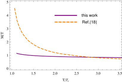
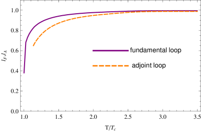
Figure 2: Left panel. Ratio $M/T$ for our model (indigo, solid line) and for the model without Polyakov loop (orange, dashed line) of Castorina:2011ra , against temperature, the latter measured in units of the critical temperature $T=270$ MeV. Right panel. Expectation value of the fundamental (indigo, solid line) and adjoint (orange, dashed line) loops against temperature. Figure adapted from Ref. Ruggieri:2012ny .

In the left panel of Fig. 2 we plot our result for the gluon mass against temperature, and we compare it with the result of Castorina:2011ra obtained without the Polyakov loop dynamics. In the right panel of the same figure we plot our results for the fundamental and the adjoint loops.

It is interesting that when the Polyakov loop is not introduced, hence within the common gluon plasma nature of the deconfinement phase, a large mass is needed to suppress pressure and energy density around $T_{c}$. As it is discussed in Castorina:2011ra , this divergence embeds the nonperturbative effects which are important at the phase transition. In our case, the statistical suppression of states below and around $T_{c}$ is achieved by virtue of the Polyakov loop, similarly to what happens in the PNJL model Fukushima:2003fw ; Ratti:2005jh ; Fukushima:2008wg ; Abuki:2008nm . For this reason, we do not need to have a large mass as $T$ approaches $T_{c}$. The nonperturbative behavior of the Polyakov loops as a function of the temperature is assured by the combined effect of the Polyakov loop effective potential, which is dominant at low temperatures and favors the confinement phase, and the quasiparticle potential, which is dominant at large temperatures and favors a nonzero expectation value of the Polyakov loops. Being the Polyakov loops different from zero, the deconfinement phase within our theoretical description is characterized by a twofold nature: a sea of background traced $Z(N)-$lines in which transverse quasiparticles propagate.

4 Conclusions

In this talk, we have summarized our recent results Ruggieri:2012ny about a combined description of the $SU(3)$ deconfinement phase, in terms of gluon quasiparticles and Polyakov loops. This picture merges the common view of the deconfinement phase as a plasma, with a picture where the relevant degrees of freedom are traced $Z(N)-$lines (Polyakov loops in fundamental as well as in higher representations) Pisarski:2006hz . Our main purpose is twofold. Firstly, we are interested to a simple description of the lattice data about the thermodynamics of the gluon plasma. This is interesting because it allows to understand which are the relevant degrees of freedom in the deconfinement phase of the theory. Moreover, once the proper degrees of freedom are identified, the effective description studied here can be completed by adding dynamical quarks. Employing a relativistic transport theory, this can allow also a direct connection between the developments of effective models and the study of the quark-gluon plasma created in relativistic heavy-ion collisions. Within our model, we are able to reproduce fairly well the lattice data about the gluon plasma thermodynamics in the critical region.

One of the main conclusions of our work is that because of the coupling to the Polyakov loop, a gluon mass of the order of the critical temperature, $m_{g}\sim 1-2\,T_{c}$, is enough to reproduce the lattice data in the critical region. This is different from what is found in standard quasi-particle models, which support the pure plasma picture of the deconfinement phase: in that case the Polyakov loops are neglected and the phase is described in terms of a perfect gas of massive gluons. As a consequence, a mass rapidly increasing with $T$ is needed to suppress pressure and energy density in the critical region. On the other hand, in the case studied in this article, the suppression of the pressure and energy density is mainly caused by the Polyakov loop. Therefore, lighter quasiparticles with a smooth $T-$dependence describe fairly well the lattice data in the critical region.

There are several interesting directions to follow to extend the present work. Firstly, having in mind the study of the quark-gluon plasma, we plan to add dynamical massive quarks to the picture. It is also of a certain interest to span the parameter space in more detail, eventually analyzing several functional forms of the gluon mass. Moreover, even in the case of the pure gauge theory, it would be interesting to investigate the way to adjust the interaction measure in order to reproduce lattice data in the regime of very large temperature. Even more, it would be of a certain interest to extend our study to the case of different gauge groups.

References

- (1) S. Datta and S. Gupta, Phys. Rev. D 82, 114505 (2010).
- (2) G. Boyd, J. Engels, F. Karsch, E. Laermann, C. Legeland, M. Lutgemeier and B. Petersson, Nucl. Phys. B 469, 419 (1996).
- (3) G. Boyd, J. Engels, F. Karsch, E. Laermann, C. Legeland, M. Lutgemeier and B. Petersson, Phys. Rev. Lett. 75, 4169 (1995).
- (4) S. .Borsanyi, G. Endrodi, Z. Fodor, S. D. Katz and K. K. Szabo, arXiv:1104.0013 [hep-ph].
- (5) S. .Borsanyi, G. Endrodi, Z. Fodor, S. D. Katz and K. K. Szabo, JHEP 1207, 056 (2012).
- (6) D.Zwanziger, Nucl. Phys. B 485(1997)185.
- (7) E. Braaten and R. D. Pisarski, Phys. Rev. D 45, R1827 (1992).
- (8) J. P. Blaizot and E. Iancu, Nucl. Phys. B 417, 608 (1994).
- (9) J. O. Andersen, E. Braaten, and M. Strickland, Phys. Rev. Lett. 83, 2139 (1999).
- (10) J. P. Blaizot, E. Iancu, and A. Rebhan, Phys. Rev. Lett. 83, 2906 (1999).
- (11) J. O. Andersen, L. E. Leganger, M. Strickland and N. Su, Phys. Lett. B 696 (2011) 468;
- (12) M. I. Gorenstein and S. N. Yang, Phys. Rev. D 52, 5206 (1995).
- (13) A. Peshier, B. Kampfer, O.P. Pavlenko and G. Soff, Phys. Rev. D54, 2399 (1996)
- (14) Levai P and Heinz U W 1998 Phys.Rev. C 57 1879
- (15) M. Bluhm, B. Kämpfer, and G. Soff, Phys. Lett. B620, 131 (2005); M. Bluhm and B. Kämpfer, Phys. Rev. D77, 114016 (2008).
- (16) M. Bluhm, B. Kampfer, K. Redlich, Nucl. Phys. A 830 (2009) 737C; M. Bluhm, B. Kampfer and K. Redlich, Phys. Lett. B 709 (2012) 77.
- (17) P. N. Meisinger, M. C. Ogilvie and T. R. Miller, Phys. Lett. B 585, 149 (2004).
- (18) P. Castorina, V. Greco, D. Jaccarino and D. Zappala, Eur. Phys. J. C 71, 1826 (2011).
- (19) F. Giacosa, Phys. Rev. D 83, 114002 (2011).
- (20) A. Peshier and W. Cassing, Phys. Rev. Lett. 94, 172301 (2005).
- (21) S. Plumari, W. M. Alberico, V. Greco and C. Ratti, Phys. Rev. D 84, 094004 (2011).
- (22) V. S. Filinov, V. E. Fortov, P. R. Levashov, Y. .B. Ivanov and M. Bonitz, Phys. Lett. A 376, 1096 (2012).
- (23) P. Castorina and M. Mannarelli, Phys. Rev. C 75, 054901 (2007); Phys. Lett. B 644, 336 (2007).
- (24) P. Castorina, D. E. Miller and H. Satz, Eur. Phys. J. C 71, 1673 (2011); P.Castorina et al., Eur. Phys. J. C66(2010)207.
- (25) F. Brau and F. Buisseret, Phys. Rev. D 79, 114007 (2009).
- (26) J. Cao, Y. Jiang, W. -m. Sun and H. -s. Zong, Phys. Lett. B 711, 65 (2012).
- (27) V. M. Bannur, Phys. Lett. B 647, 271 (2007); V. M. Bannur, Eur. Phys. J. C 50, 629 (2007);
- (28) F. Scardina, M. Colonna, S. Plumari and V. Greco, arXiv:1202.2262 [nucl-th]. Plumari S, Baran V, Di Toro M, Ferini G and Greco V 2010 Phys.Lett. B 689 18
- (29) A. M. Polyakov, Phys. Lett. B 72, 477 (1978).
- (30) L. Susskind, Phys. Rev. D 20, 2610 (1979).
- (31) B. Svetitsky and L. G. Yaffe, Nucl. Phys. B 210, 423 (1982).
- (32) B. Svetitsky, Phys. Rept. 132, 1 (1986).
- (33) K. Fukushima, Phys. Lett. B 591, 277 (2004).
- (34) C. Ratti, M. A. Thaler and W. Weise, Phys. Rev. D 73, 014019 (2006).
- (35) H. Abuki and K. Fukushima, Phys. Lett. B 676, 57 (2009).
- (36) T. Zhang, T. Brauner and D. H. Rischke, JHEP 1006, 064 (2010).
- (37) S. Gupta, K. Huebner and O. Kaczmarek, Phys. Rev. D 77, 034503 (2008).
- (38) N. Weiss, Phys. Rev. D 24, 475 (1981).
- (39) K. Fukushima, Phys. Rev. D 77, 114028 (2008) [Erratum-ibid. D 78, 039902 (2008)].
- (40) H. Abuki, R. Anglani, R. Gatto, G. Nardulli and M. Ruggieri, Phys. Rev. D 78, 034034 (2008).
- (41) C. Sasaki and K. Redlich, arXiv:1204.4330 [hep-ph].
- (42) M. Ruggieri, P. Alba, P. Castorina, S. Plumari, C. Ratti and V. Greco, arXiv:1204.5995 [hep-ph].
- (43) J. Braun, H. Gies and J. M. Pawlowski, Phys. Lett. B 684, 262 (2010); J. Braun, A. Eichhorn, H. Gies and J. M. Pawlowski, Eur. Phys. J. C 70, 689 (2010); J. Braun and A. Janot, Phys. Rev. D 84, 114022 (2011).
- (44) J. O. Andersen, M. Strickland and N. Su, JHEP 1008, 113 (2010).
- (45) J. O. Andersen, M. Strickland and N. Su, Phys. Rev. Lett. 104, 122003 (2010).
- (46) R. D. Pisarski, Phys. Rev. D 74, 121703 (2006); Phys. Rev. D 62, 111501 (2000); A. Dumitru, Y. Guo, Y. Hidaka, C. P. K. Altes and R. D. Pisarski, arXiv:1205.0137 [hep-ph].