Size measurement of dynamically generated resonances with finite boxes

Abstract

The structure of dynamically generated states is studied from a viewpoint of the finite volume effect. We establish the relation between the mean distance between constituents inside a stable bound state and the finite volume mass shift. In a single-channel scattering model, this relation is shown to be valid for a bound state dominated by the two-body molecule component. We generalize this method to the case of a quasi-bound state with finite width in coupled-channel scattering. We define the real-valued mean distance between constituents inside the resonance in a given closed channel using the response to the finite volume effect on the channel. Applying this method to physical resonances we find that $\Lambda(1405)$ and $f_{0}(980)$ are dominated by the $\bar{K}N$ and $K\bar{K}$ scattering states, respectively, and that the distance between $\bar{K}N$ ($K\bar{K}$) inside $\Lambda(1405)$ [$f_{0}(980)$] is $1.7$–$1.9\text{ fm}$ ($2.6$–$3.0\text{ fm}$). The root mean squared radii of $\Lambda(1405)$ and $f_{0}(980)$ are also estimated from the mean distance between constituents.

I Introduction

There are several hadrons which are expected to have some exotic structures (exotic hadrons), and clarifying structures of these exotic hadrons is one of the important tasks for the study of the strong interactions Nakamura:2010zzi . A classic example of exotic hadrons is the hyperon resonance $\Lambda(1405)$, which is the lightest baryon with spin-parity $J^{P}=1/2^{-}$ although containing one strange quark. This resonance has been considered as a quasi-bound state of the $\bar{K}N$ system Dalitz:1960du ; Dalitz:1967fp owing to the strongly attractive $\bar{K}N$ interaction in the $I=0$ channel. Another example is found in the lightest scalar meson nonet [$f_{0}(600)=\sigma$, $\kappa(800)$, $f_{0}(980)$, and $a_{0}(980)$], which exhibits an inverted spectrum from the naïve expectation with the $q\bar{q}$ assignment. There are several attempts to explain this anomaly, e.g., multiquark configurations for the scalar nonet Jaffe:1976ig ; Jaffe:1976ih and $K\bar{K}$ molecules for $f_{0}(980)$ and $a_{0}(980)$ Weinstein:1982gc ; Weinstein:1983gd . Recently $\Lambda(1405)$ and the lightest scalar mesons are successfully described by coupled-channel chiral dynamics (chiral unitary approach) in meson-baryon Kaiser:1995eg ; Oset:1997it ; Oller:2000fj ; Lutz:2001yb ; Hyodo:2011ur and meson-meson Dobado:1993ha ; Oller:1997ti ; Oller:1998hw scatterings, respectively.

One of the characteristic features of exotic hadrons is the spatial size, because one expects larger size of hadronic molecules than ordinary hadrons. However, in general, candidates of exotic hadrons are not in ground states but resonances with finite decay width. Because of the decay process, mean squared radius of a resonance is obtained as a complex number whose interpretation is not straightforward Sekihara:2008qk ; Sekihara:2010uz . To overcome this difficulty, we recall the finite volume effect on bound states. It has been shown in Refs. Luscher:1985dn ; Beane:2003da ; Koma:2004wz ; Sasaki:2006jn ; Davoudi:2011md that the binding energy increases when a bound state of two particles is confined in a finite box with periodic boundary condition. The reason is that the wave function of the bound state in the box penetrates to the adjacent box and hence the expectation value of the potential energy grows negatively. This means that the finite volume effect is closely related with the spatial structure of the bound state.

Motivated by these observations, in this study we aim at establishing the relation between the finite volume effect and the spatial size of both stable bound states and unstable resonance states, or more precisely the mean distance between constituents inside the bound and resonance states. Firstly, we consider a stable bound state in single-channel scattering where the mean distance between constituents is well defined. We develop a method to evaluate the mean distance from the finite volume effect, and examine its validity using a dynamical scattering model. This method is straightforwardly generalized to a bound state in coupled-channel scattering. In this case, the size of the bound state is defined for each channel, which can be estimated by the finite volume effect on the channel of interest, with the other channels being unchanged. Next we extend this method to a resonance state in coupled-channel scattering, and estimate the mean distance between constituents of the resonance in closed channels. As applications to physical states, we examine the coupled-channel models for $\Lambda(1405)$ and the scalar mesons $\sigma$, $f_{0}(980)$, and $a_{0}(980)$ to elucidate their structures.

This paper is organized as follows. In Sec. II we formulate the size measurement of (quasi-)bound states using the finite volume effect, and introduce a dynamical scattering model. In Sec. III we examine the validity of our strategy using the finite volume effect in the case of single-channel bound state, and apply the method to physical hadron resonances. Section IV is devoted to the conclusion of this study.

II Formulation

II.1 Size measurement with finite volume effect

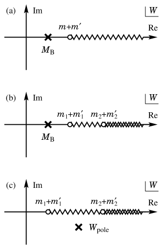
Figure 1: Schematic figure of (quasi-)bound state poles and continuum states in the complex plane of energy $W$. (a) A bound state in single-channel scattering, (b) a bound state in coupled-channel scattering, and (c) a quasi-bound state in coupled-channel scattering.

Here we present the basic idea to determine the mean distance between constituents inside the (quasi-)bound state from the mass shift due to the finite volume effect. The mean distance between constituents inside the bound state is straightforwardly related to the size of the system when the spatial size of constituents is negligible compared to the distance between constituents. Let us first consider the simplest case: a bound state with mass $M_{\rm B}$ in the single-channel scattering of particles with masses $m$ and $m^{\prime}\leq m$ [see Fig. 1 (a)]. In nonrelativistic quantum mechanics, the mean squared distance of two particles in an weakly bound state can be read off from the tail of the wave function as Sekihara:2010uz

$$\langle r^{2}\rangle_{\text{NR}}= \frac{1}{4\mu B_{\rm{E}}},$$ (1)

with the reduced mass $\mu=mm^{\prime}/(m+m^{\prime})$ and the binding energy $B_{\rm{E}}=m+m^{\prime}-M_{\rm B}$. At first glance, the mean squared distance for the bound state seems to be solely determined by the mass of the bound state. However, it is implicitly assumed in Eq. (1) that the bound state is completely described by the model space of the two-body scattering. In field theory, in addition to the scattering state, there can be a “bare state” contribution (elementarity) whose fraction in the physical bound state is expressed by the wave function renormalization constant $Z$ Weinberg:1965zz ; PR136.B816 . The mean squared distance for the bound state, which stems from the scattering state contribution, should then be given by subtracting the bare state contribution as

$$\langle r^{2}\rangle= \frac{1-Z}{4\mu B_{\rm{E}}},$$ (2)

where the factor $1-Z$ is called the compositeness. As shown in Refs. Weinberg:1965zz ; PR136.B816 ; Hyodo:2011qc , the compositeness is related with the coupling constant of the physical bound state to the two-body scattering state $g$:

$$1-Z= -g^{2}G^{\prime}(M_{\rm B}^{2}),\quad G^{\prime}(s)=\frac{dG(s)}{ds},$$ (3)

where $G$ is the two-body loop integral as a function of squared energy $s\equiv W^{2}$ to be specified below. Thus, the mean squared distance for the bound state is expressed in terms of the mass $M_{\rm B}$ and its coupling to the scattering state $g$.

At this point we make use of the finite volume effect on the mass of a bound state studied in Refs. Luscher:1985dn ; Beane:2003da ; Koma:2004wz ; Sasaki:2006jn ; Davoudi:2011md . When a bound state is put in a periodic finite box of size $L$, the mass $M_{\rm B}$ is shifted to $\tilde{M}_{\rm B}(L)$, and the mass shift $\Delta M_{\rm B}(L)\equiv\tilde{M}_{\rm B}(L)-M_{\rm B}$ is related to the coupling constant $g$. As shown in Appendix A, the leading contribution to the mass shift formula in the present case is given by

$$\Delta M_{\rm B}(L)= -\frac{3g^{2}}{8\pi M_{\rm B}^{2}L}\exp\left[-\bar{\mu}L\right]+\mathcal{O}(e^{-\sqrt{2}\bar{\mu}L}),$$ (4)

$$\bar{\mu}= \frac{\sqrt{-\lambda(M_{\rm B}^{2},\,m^{2},\,m^{\prime 2})}}{2M_{\rm B}},$$ (5)

where $\lambda(x,\,y,\,z)=x^{2}+y^{2}+z^{2}-2xy-2yz-2zx$ is the Källen function. An important point is that the leading contribution depends on $g^{2}$ and $M_{\rm B}$ in the infinite volume. Namely, we can read off the physical coupling constant $g$ from the $L$ dependence of the mass of the bound state. Equations (2) and (3) show that the bound state has large mean squared distance when the coupling $g$ is large. This fact is intuitively understood in Eq. (4) by the $g^{2}$ factor; a bound state with large mean squared distance (and thus the large coupling $g$) has strong finite volume effect. In other words, the structure of the bound state is quantitatively reflected in the finite volume effect. We also note that the factor $\bar{\mu}$ represents virtuality of the constituent particles inside the bound state.

Equation (4) provides us an alternative strategy to estimate the mean squared distance for a bound state. Suppose that we are able to calculate the mass shift $\Delta M_{\rm B}(L)$ of the bound state in finite volume at large $L$. In this case, using the mass shift formula (4) up to the leading order, we determine the coupling strength $g_{\rm FV}$. The mean squared distance is then evaluated as

$$\langle r^{2}\rangle_{\rm FV}=\frac{-g_{\rm FV}^{2}G^{\prime}(M_{\rm B}^{2})}{4\mu B_{\rm{E}}}.$$ (6)

If the $L$ dependence of the mass shift is correctly fitted by Eq. (4), we expect $g_{\rm FV}\to g$ and $\langle r^{2}\rangle_{\rm FV}\to\langle r^{2}\rangle$. In this way, the mean squared distance for the bound state is related with the finite volume mass shift at large $L$.

The virtue of this new approach will become clear when the argument is extended to the quasi-bound state with finite width. To this end, we begin with the case of a bound state in multichannel scattering as shown in Fig. 1 (b). Labeling the scattering states by the suffix $i$, we can decompose the bound state wave function into the bare state contribution ($Z$) and the contribution from the scattering state in channel $i$ ($X_{i}$) Hyodo:2011qc , which are normalized as

$$1= Z+\sum_{i}X_{i},$$ (7)

$$X_{i}= -g_{i}^{2}G_{i}^{\prime}(M_{\rm{B}}^{2}).$$ (8)

In this case, the mean squared distance of the bound state in channel $i$ is defined as

$$\langle r^{2}\rangle_{i}= \frac{-g_{i}^{2}G_{i}^{\prime}(M_{\rm{B}}^{2})}{4\mu_{i}B_{\text{E},i}},$$ (9)

with $g_{i}$ being the coupling constant to channel $i$, $B_{\text{E},i}=m_{i}+m^{\prime}_{i}-M_{\rm{B}}$ and $\mu_{i}=m_{i}m^{\prime}_{i}/(m_{i}+m^{\prime}_{i})$. Conceptually, $\langle r^{2}\rangle_{i}$ corresponds to the mean squared distance measured by the probe current which exclusively couples to the component in channel $i$. Then the coupling constant $g_{i,\rm{FV}}$ can be extracted from the mass shift by putting only the channel $i$ in the finite box with size $L$ and keeping the other channels unchanged. Substituting this coupling constant $g_{i,\rm{FV}}$ into Eq. (9), we obtain $\langle r^{2}\rangle_{i,\rm{FV}}$.

We can further extend this argument to a quasi-bound state with finite width. Consider a system with two coupled channels in which the higher energy channel has a bound state when the transition potential is switched off. The bound state acquires a decay width through the channel coupling to the lower energy channel, which is called a quasi-bound state or a Feshbach resonance [see Fig. 1 (c)]. In this case, the pole of the resonance locates in the complex energy plane at total energy $W=W_{\text{pole}}$. If the channel coupling is not strong, the imaginary part of the pole position is small and we can identify the real part as the “mass” of the state, $M_{\rm{B}}\equiv\text{Re}[W_{\text{pole}}]$. Applying the same procedure, we determine the coupling constant $g_{i,\rm{FV}}$ from the $L$ dependence of the real part of the resonance pole when the channel $i$ is put in the box. Substituting it in Eq (9), we estimate the mean squared distance for the quasi-bound state. The binding energy as well as the loop integral are evaluated at this energy $M_{\rm{B}}\equiv\text{Re}[W_{\text{pole}}]$. Note that this is only applicable to the closed channels, namely, the resonance pole should be located below the threshold of channel $i$. If we put an open channel in the finite box, the continuum state of that channel is discretized and we cannot perform the analytic continuation to the complex energy plane.

It is important that this procedure gives a real-valued $\langle r^{2}\rangle_{i}$ of the quasi-bound state, since the coupling extracted from Eq. (4) is a real number. In general, it is known that the mean squared radius Sekihara:2008qk ; Sekihara:2010uz and compositeness Hyodo:2011qc become complex in the case of resonances, which are difficult to interpret. The strategy presented here can provide an alternative way to investigate the structure of resonances.

Before closing this section, we comment on the modifications of the formulation due to the finite size of the constituent particles. As discussed in Appendix A, the mass shift of the constituent particles are in the higher order than the leading contribution (4), so this effect can be neglected at least with sufficiently large $L$. As a consequence, up to the leading order, in which we are considering here, our formulation will not be modified even if the constituent particles have their own spatial structures. Nevertheless, although the spatial structure of the constituents does not affect the separation between constituents in this study, mean squared radius of the whole system becomes larger when the spatial structures of the constituents are taken into account (see Appendix B).

In the following, we introduce a hadron scattering model together with finite volume effect, in order to examine the size measurement with finite box.

II.2 Coupled-channel scattering model and finite volume effect

Here we formulate a model to describe stable bound states and unstable resonance states along the line with Ref. Oller:2000fj . We prepare a coupled-channel interaction kernel $V_{ij}$ and evaluate the scattering amplitude $T_{ij}$ by the Bethe-Salpeter equation in its factorized form:

$$T_{ij}(s)=V_{ij}+\sum_{k}V_{ik}G_{k}T_{kj}=\sum_{k}{(1-VG)^{-1}}_{ik}V_{kj},$$ (10)

where indices $i$, $j$, and $k$ represent the scattering channels, $s\equiv W^{2}$ is the squared center-of-mass energy of the scattering system. The explicit form of $V_{ij}$ will be given in the next section. $G_{k}$ is the loop integral,

$$G_{k}(s)=i\int\frac{d^{4}q}{(2\pi)^{4}}\frac{1}{q^{2}-m_{k}^{2}+i\epsilon}\frac{1}{(P-q)^{2}-m_{k}^{\prime 2}+i\epsilon},$$ (11)

with $m_{k}$, $m_{k}^{\prime}$, and $P^{\mu}=(W,\bm{0})$ being the masses of the particles in channel $k$ and the four-momentum of the two-body system, respectively. Using the dimensional regularization, one can rewrite the loop integral as

$$G_{k}(s)= \frac{1}{16\pi^{2}}\Bigg{[}a_{k}(\mu_{\rm reg})+\ln\frac{m_{k}^{2}}{\mu_{\rm reg}^{2}}+\frac{m_{k}^{\prime 2}-m_{k}^{2}+s}{2s}\ln\frac{m_{k}^{\prime 2}}{m_{k}^{2}}$$

$$+\frac{\sqrt{\lambda_{k}}}{2s}\Big{\{}\ln(s-m_{k}^{2}+m_{k}^{\prime 2}+\sqrt{\lambda_{k}})$$

$$\phantom{+\frac{q_{k}}{\sqrt{s}}\Big{\{}}+\ln(s+m_{k}^{2}-m_{k}^{\prime 2}+\sqrt{\lambda_{k}})$$

$$\phantom{+\frac{q_{k}}{W}\Big{\{}}-\ln(-s+m_{k}^{2}-m_{k}^{\prime 2}+\sqrt{\lambda_{k}})$$

$$\phantom{+\frac{q_{k}}{W}\Big{\{}}-\ln(-s-m_{k}^{2}+m_{k}^{\prime 2}+\sqrt{\lambda_{k}})\Big{\}}\Bigg{]},$$ (12)

with the regularization scale $\mu_{\rm reg}$, the subtraction constant $a_{k}$, and $\lambda_{k}\equiv\lambda(s,\,m_{k}^{2},\,m_{k}^{\prime 2})$. We note that the regularization scale and the subtraction constant are not independent, and the subtraction constant is a single parameter of the loop function in each channel.

Bound states and resonance states appear as poles in the scattering amplitude $T_{ij}$ as

$$T_{ij}(s)=\frac{g_{i}g_{j}}{s-s_{\rm pole}}+T_{ij}^{\rm BG}(s),$$ (13)

where the background term $T_{ij}^{\rm BG}$ is chosen to make the product $g_{i}g_{j}$ energy independent. The constant $g_{i}$ can be interpreted as the coupling strength of the state to the channel $i$. The pole position $s_{\rm pole}$ is a solution of the equation,

$$\det(1-VG)=0,$$ (14)

which is simplified as $V^{-1}=G$ in the single-channel case. A stable bound state is represented by a pole on the real axis of the first Riemann sheet below the threshold, while an unstable resonance state corresponds to a pole in the complex lower-half plane of the second Riemann sheet above the threshold.

In this model, we have a relation,

$$-\sum_{i,j}\left[g_{i}\frac{dG_{i}}{ds}g_{i}\delta_{ij}+g_{i}G_{i}\frac{dV_{ij}}{ds}G_{j}g_{j}\right]_{s\to s_{\rm pole}}=1,$$ (15)

which is the generalized Ward identity Sekihara:2010uz ; Hyodo:2011qc ; Aceti:2012dd . With Eq. (8), we can identify the first term as the sum of the contributions from hadronic composite states. It follows from Eq. (7) that the bare pole contribution $Z$ is expressed by the second term as

$$Z=-\sum_{i,j}g_{i}G_{i}\frac{dV_{ij}}{ds}G_{j}g_{j}\Bigg{|}_{s\to s_{\rm pole}}.$$ (16)

In Ref. Hyodo:2011qc $Z$ is shown to be exactly the bare pole contribution for stable bound states, and thus for unstable resonance states the system is expected to have less compositeness as $Z$ approaches unity.

Next we consider the finite volume effect in a spatial box with size $L$. In general, the finite volume effect appears as the discretized momentum in the loop function Luscher:1986pf . The finite volume effect in the present model has been discussed in Refs. Doring:2011vk ; MartinezTorres:2011pr by using discretized momentum loop function $\tilde{G}_{i}$,

$$\tilde{G}_{i}(s)=\frac{i}{L^{3}}\sum_{\bm{q}}\int\frac{dq^{0}}{2\pi}\frac{1}{q^{2}-m_{i}^{2}}\frac{1}{(P-q)^{2}-m_{i}^{\prime 2}},$$

$$\bm{q}=\frac{2\pi\bm{n}}{L},\quad\bm{n}\in\mathbb{Z}^{3},$$ (17)

instead of the loop integral $G_{i}$ in Eq. (10). Here, we evaluate $\tilde{G}_{i}$ with the dimensional regularization following Ref. MartinezTorres:2011pr by extracting three-dimensional integral from $G_{i}$ and replace it with the summation with discretized momentum, which results in,

$$G_{i}(s)\to\tilde{G}_{i}(s)=G_{i}(s)$$

$$+\lim_{q_{\rm max}\to\infty}\left(\frac{1}{L^{3}}\sum_{\bm{q}}^{|\bm{q}|<q_{\rm max}}I_{i}(s,q)-\int_{q<q_{\rm max}}\frac{d^{3}q}{(2\pi)^{3}}I_{i}(s,q)\right),$$ (18)

with

$$I_{i}(s,q)=\frac{1}{2\omega_{i}\omega_{i}^{\prime}}\frac{\omega_{i}+\omega_{i}^{\prime}}{s-(\omega_{i}+\omega_{i}^{\prime})^{2}},$$ (19)

$$\omega_{i}(q)=\sqrt{q^{2}+m_{i}^{2}},\quad\omega_{i}^{\prime}(q)=\sqrt{q^{2}+m_{i}^{\prime 2}}.$$ (20)

It is known that, with finite cut-off $q_{\rm max}$, $\tilde{G}_{i}$ exhibits oscillations which gradually vanish as $q_{\rm max}$ goes to infinity MartinezTorres:2011pr . This oscillation is caused by the summation over the discretized momentum, which is not a continuous function of $q_{\rm{max}}$. The absolute value of the integrand $I_{i}(s,q)$ decreases for large $q$, so the discontinuity becomes small with large $q_{\rm{max}}$. In order to make convergence with respect to the oscillation, following Ref. MartinezTorres:2011pr , we will take averaged value of $\tilde{G}_{i}$ within range $q_{\rm max}\in[2\text{ GeV},\,4\text{ GeV}]$ in the numerical calculation.

When we put all the channels in the finite box, momenta of the scattering states above the threshold are also discretized, and the eigenenergies are constrained by the pole condition Doring:2011vk

$$\det(1-V\tilde{G})=0,$$ (21)

which again reduces to $V^{-1}=\tilde{G}$ in the single-channel case. Note that for bound state poles below the threshold, Eq. (14) and Eq. (21) are the same condition with different loop function. For the application to the quasi-bound state, we will use the loop function with channel $i$ in the finite box as

$$G=\begin{pmatrix}G_{1}&&&&\\ &G_{2}&&&\\ &&\ddots&&\\ &&&\tilde{G}_{i}&\\ &&&&\ddots\end{pmatrix}.$$ (22)

In this case, if the energy is smaller than the threshold of channel $i$, $W<m_{i}+m^{\prime}_{i}$, the scattering amplitude $T=(V^{-1}-G)^{-1}$ is a continuous function of $W$, and the resonance pole can be searched for through the analytic continuation of the amplitude in a usual manner.

III Results

III.1 Size of bound states in single-channel scattering

Now let us consider stable bound states in single-channel scattering and see how they behave in the finite volume. In Sec. II.1, we have presented two methods to calculate the mean squared distance between constituents inside the bound state. The mean squared distance in Eq. (2) is obtained from the residue of the pole, and that in Eq. (6) is evaluated by the finite volume effect. In addition, the corresponding mean squared distance can also be calculated by using the response to an external probe current as shown in Ref. Sekihara:2010uz . Comparing the results from different methods, we examine the validity of the size estimation.

In this subsection, with the $\bar{K}N$ system in mind, we choose the masses in the scattering state as $m=938.9\text{ MeV}$ and $m^{\prime}=495.7\text{ MeV}$, respectively. We use the natural subtraction constant $a=-1.95$ with the regularization scale $\mu_{\rm reg}=630\text{ MeV}$, which is obtained to exclude explicit pole contributions from the loop integral Hyodo:2008xr . For the interaction kernel $V$ we consider two types. One is the constant interaction,

$$V_{\rm I}=v_{0},$$ (23)

with the energy independent parameter $v_{0}$ (case I). The other interaction consists of a bare pole term,

$$V_{\rm II}=\frac{g_{0}^{2}}{s-s_{0}},$$ (24)

with two parameters $g_{0}$ and $s_{0}$ which are constrained by $g_{0}=\sqrt{s_{0}}$ for simplicity (case II). The parameters $v_{0}$ and $g_{0}=\sqrt{s_{0}}$ are fixed so as to produce a bound state with binding energy $B_{\rm E}=10\text{ MeV}$ in both cases, and as a result we have $v_{0}=124.9$ and $g_{0}=\sqrt{s_{0}}=1.430\text{ GeV}$.

Table 1: Properties of bound states in cases I and II. The results in column “Pole” are calculated from the residue of the pole in the models, and those in “Finite Volume” are obtained by using the finite volume effect.

Case I	Pole	Finite Volume
$g$	$5.42\text{ GeV}$	$5.2$ – $5.8\text{ GeV}$
$Z$	$0$	$-0.14$ – $0.09$
$1-Z$	$1$	$\phantom{-}0.91$ – $1.14$

Case II	Pole	Finite Volume
$g$	$1.38\text{ GeV}$	$1.7$ – $2.6\text{ GeV}$
$Z$	$0.935$	$0.78$ – $0.90$
$1-Z$	$0.065$	$0.10$ – $0.22$

Properties of the bound states in two cases I and II are summarized in the second column of Table 1. The coupling constant $g$ is calculated from the residue of the bound state pole as in Eq. (13), and the bare pole contribution $Z$ is obtained by Eq. (16). As one can see from Table 1, the bound state by the constant interaction in case I has $Z=0$ Hyodo:2011qc , which can be understood by Eq. (16). On the other hand, the bare pole potential creates large elementarity $Z=0.935$ in case II. Purely elementary state with $Z=1$ can be obtained by taking the limit $g_{0}\to 0$ and $s_{0}\to M_{\rm B}^{2}$ with fixed $B_{\rm E}$.

Table 2: Mean distance between constituents inside bound states in cases I and II with several methods.

	Eq. (2)	Probe Sekihara:2010uz	Eq. (6)
Case I, $\sqrt{\langle r^{2}\rangle}$ [fm]	$1.73$	$1.86$	$1.7$ – $1.8$
Case II, $\sqrt{\langle r^{2}\rangle}$ [fm]	$0.44$	$0.48$	$0.5$ – $0.8$

With the obtained compositeness $1-Z$ and Eq. (2), we calculate the mean distance for the bound state as shown in the second column of Table 2. Here we also calculate the mean distance using probe method developed in Ref. Sekihara:2010uz , in which the external probe current is coupled to the particles in the scattering state and the mean squared distance is obtained from the form factor. The results are shown in the third column of Table 2. Comparing two cases, we observe that the bound state in case I has large separation between constituents $\sqrt{\langle r^{2}\rangle}\sim 1.8\text{ fm}$ compared to the hadronic scale $\lesssim 0.8\text{ fm}$, whereas in case II the separation for the bound state is $\sqrt{\langle r^{2}\rangle}\sim 0.5\text{ fm}$. This is because only the two-particle cloud can contribute to the mean distance. These results indicate that the mean distance for the bound state is not exclusively determined by its binding energy, and the magnitude of the coupling constant is closely related with the internal structure, as discussed in Sec. II.1.

Figure 2: The loop integrals in infinite and finite volume, $G$ and $\tilde{G}$, and inverse of the interaction $V_{\rm I}$ and $V_{\rm II}$ as functions of $W\equiv\sqrt{s}$. Vertical dotted line represents the threshold of the two-body system, $W=m+m^{\prime}$.

For later convenience, the loop integral $G$ and the inverse of the interaction kernels $V_{\rm I}^{-1}$ and $V_{\rm II}^{-1}$ are plotted as functions of $W\equiv\sqrt{s}$ in Fig. 2. Below the threshold, the loop function $G$ is real. In this figure, the intersection point of $G$ and $V^{-1}$ corresponds to the mass of the bound state $M_{\rm B}$ according to Eq. (14). In both cases the intersection appears at $M_{\rm B}=1424.6\text{ MeV}$ with the binding energy $B_{\rm E}=10\text{ MeV}$ with the adopted parameters. An important point to note here is that the energy dependence of two interaction kernels is very different from each other. While $V_{\rm I}^{-1}$ is completely flat, $V_{\rm II}^{-1}$ is almost vertical with steep slope. In the limit of $g_{0}\to 0$ and $s_{0}\to M_{\rm{B}}^{2}$, the slope becomes completely vertical. This difference of the interaction kernel will be crucial to the finite volume effect on the bound states.

Then let us take into account the finite volume effect by replacing the loop integral $G$ with that in finite volume $\tilde{G}$. Behavior of $\tilde{G}$ is also plotted in Fig. 2 with box sizes $L=4.0$, $5.0$ and $6.0\text{ fm}$. Because of the pole condition (21), the mass of the bound state in finite volume $\tilde{M}_{\rm{B}}(L)$ corresponds to the intersection point of $\tilde{G}$ and $V^{-1}$. From Fig. 2, one observes that in both cases the mass of the bound state decreases when the box size $L$ decreases. However, $L$ dependence of the mass of the bound state is quantitatively different in two cases. The flat (steep) energy dependence of $V_{\rm{I}}^{-1}$ ($V_{\rm{II}}^{-1}$) results in the strong (mild) $L$ dependence of the bound state mass in finite volume. Different $L$ dependence of the mass shift in two cases is understood by this geometric argument.

Figure 3: The mass shift of the bound states with two interactions $\Delta M_{\rm B}=\tilde{M}_{\rm B}-M_{\rm B}$ as a function of $L$. The prediction by the mass shift formula (4) is also plotted.

To compare with the mass shift formula (4), we plot in Fig. 3 the mass shift $\Delta M_{\rm B}(L)=\tilde{M}_{\rm{B}}(L)-M_{\rm{B}}$ as a function of $L$. From this figure, we observe the decrease of the mass for the smaller box size $L$ in both cases I and II. Furthermore, one can see the rapid decrease of the mass in case I compared to that in case II. This can be interpreted as the consequence of the loose binding of the system (large mean squared distance) in case I.

Using the coupling constant obtained from the pole residue, we can predict the mass shift $\Delta M_{\rm B}$ by Eq. (4) which is plotted in Fig. 3. With large $L$, the formula (4) well reproduces the mass shift, but some deviation becomes evident in smaller $L$ region especially for the case II. This means that higher order corrections on the mass shift formula is necessary to describe finite volume effect of the bound state. In fact, since the coupling $g$ is small in the case II, it is reasonable that the higher order correction to the mass shift formula is more important than the case I.

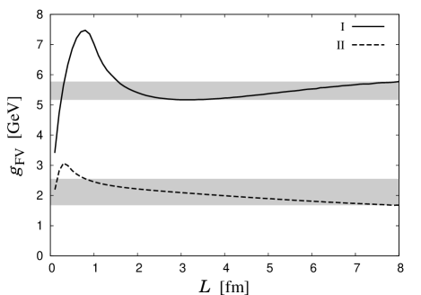
Figure 4: Coupling strength evaluated by Eq. (25) as a function of $L$. The bands show the adopted values of $g_{\rm FV}$ in our study for both cases I and II.

Let us extract the bound state properties by using the finite volume effect in the procedure of Sec. II.1. Fitting the mass shift by the formula (4), we evaluate the coupling strength $g_{\rm FV}$, the bare pole contribution $Z_{\rm FV}$, and mean squared distance $\langle r^{2}\rangle_{\rm FV}$. In this study we take the following strategy to evaluate the coupling strength $g_{\rm FV}$. Namely, since the mass of the bound state is expected to change according to Eq. (4) at the leading order, the coupling strength $g_{\rm FV}$ can be extracted by the fraction of the mass shift obtained in our model, $\Delta M_{\rm B}(L)$, and the factor $-3\exp(-\bar{\mu}L)/(8\pi M_{\rm B}^{2}L)$ as,

$$g_{\rm FV}=\sqrt{\frac{\Delta M_{\rm B}(L)}{\displaystyle-\frac{3}{8\pi M_{\rm B}^{2}L}\exp\left[-\bar{\mu}L\right]}},$$ (25)

with

$$\bar{\mu}=\frac{\sqrt{-\lambda(M_{\rm B}^{2},\,m^{2},\,m^{\prime 2})}}{2M_{\rm B}}.$$ (26)

This $g_{\rm FV}$ depends on the box size $L$ especially in small $L$ region where the higher order contributions are not negligible. Nevertheless, we expect that $g_{\rm FV}$ in Eq. (25) becomes almost flat in the region where the mass shift is dominated by the leading order contribution. In Fig. 4 we plot $g_{\rm FV}$ in Eq. (25) as a function of the box size $L$ for both cases I and II. From the figure, we can see that $g_{\rm FV}$ in case I is fairly flat at $L\sim 3\text{ fm}$, while it rapidly changes below $\sim 2\text{ fm}$ due to the higher order contributions to the mass shift. On the other hand, in case II $g_{\rm FV}$ increases without flat regions as $L$ decreases down to $\sim 1\text{ fm}$. Here in order to determine the fairly flat region we make a criterion as follows. Namely, according to Eqs. (4) and (13), the typical scales of the box size $L$ and the coupling strength $g$ are of the order of $1/\bar{\mu}$ and $M_{\rm B}=\sqrt{s_{\rm pole}}$, respectively. Therefore, the typical scales in Fig. 4 are respectively $1/\bar{\mu}$ and $M_{\rm B}$ for the horizontal and vertical axes. These characteristic scales can make a model independent criterion $|dg_{\rm FV}/dL|<\bar{\mu}M_{\rm B}$ for the fit range to be fairly flat $g_{\rm FV}(L)$. This fit range corresponds to $L\in[1.9\text{ fm},\,8.0\text{ fm}]$ and $[0.8\text{ fm},\,8.0\text{ fm}]$ in case I and II, respectively, with $\bar{\mu}M_{\rm B}=0.58\text{ GeV}/\text{fm}$, and adopt $g_{\rm FV}$ in these ranges as the coupling strength from the finite volume effect. The adopted values of $g_{\rm FV}$ is shown as bands in Fig. 4 for both cases I and II. The results are summarized in Tables 1 and 2. As a result, we qualitatively reproduce the structure of the bound state. Especially the properties of the bound state in case I are reproduced within $\sim 10\%$ accuracy. This indicates that the measurement of mean distance between constituents with the finite volume effect is a powerful tool to clarify the structure of bound states which have dynamical origin.

III.2 Application to physical resonances

In the previous subsection we have developed a method to estimate the separation between constituents inside the bound state by using the finite volume effect. One of the important features of our procedure is the applicability to Feshbach resonance states with finite widths as discussed in Sec. II.1. Furthermore, one can obtain real-valued distance between constituents for the resonance states with respect to a closed channel. In this subsection we use this method to discuss the structure of physical hadronic resonance states from the finite volume.

Let us discuss $\Lambda(1405)$ in $\bar{K}N$-$\pi\Sigma$-$\eta\Lambda$-$K\Xi$ coupled-channels and $\sigma$, $f_{0}(980)$, and $a_{0}(980)$ scalar mesons in $\pi\pi$-$\pi\eta$-$K\bar{K}$ coupled-channels, assuming the isospin symmetry. These resonances have been studied in chiral unitary approach Kaiser:1995eg ; Oset:1997it ; Oller:2000fj ; Lutz:2001yb ; Hyodo:2011ur ; Dobado:1993ha ; Oller:1997ti ; Oller:1998hw , which is now elaborated using next-to-leading order chiral interactions with recent experimental data Ikeda:2011pi ; Ikeda:2012au ; GomezNicola:2001as . To concentrate on the size estimation with the finite volume effect, here we utilize simplified models with leading order interactions as follows. For $\Lambda(1405)$ we employ the Weinberg-Tomozawa term as the interaction kernel,

$$V_{ij}=-\frac{C_{ij}}{4f^{2}}(2W-M_{i}-M_{j})\sqrt{4M_{i}M_{j}},$$ (27)

with $M_{i}$ being the baryon mass in channel $i$, $f$ the meson decay constant, and $C_{ij}$ the Clebsch-Gordan coefficient which is determined by the $\text{SU}(3)$ group structure of the interaction,

$$C_{ij}=\left(\begin{array}[]{@{\,}cccc@{\,}}3&-\sqrt{3/2}&3/\sqrt{2}&0\\ -\sqrt{3/2}&4&0&\sqrt{3/2}\\ 3/\sqrt{2}&0&0&-3/\sqrt{2}\\ 0&\sqrt{3/2}&-3/\sqrt{2}&3\end{array}\right),$$ (28)

where $i=1$, $2$, $3$, and $4$ denote the $\bar{K}N$, $\pi\Sigma$, $\eta\Lambda$, and $K\Xi$ channels, respectively. The meson decay constant is $f=1.123f_{\pi}$ with $f_{\pi}=93.0\text{ MeV}$. The subtraction constant is $a_{1}=-1.84$, $a_{2}=-2.00$, $a_{3}=-2.25$, and $a_{4}=-2.67$ with the regularization scale $\mu_{\rm reg}=630\text{ MeV}$ in all meson-baryon channels Oset:2001cn . For the scalar meson case, we take the lowest order $s$-wave meson-meson interaction in chiral perturbation theory as the interaction kernel, namely,

$$V_{11}=\frac{m_{\pi}^{2}-2s}{2f_{\pi}^{2}},\quad V_{12}=V_{21}=-\frac{\sqrt{3}s}{4f_{\pi}^{2}},\quad V_{22}=-\frac{3s}{4f_{\pi}^{2}},$$ (29)

for the $I=0$ channel with $i=1$ ($2$) for $\pi\pi$ ($K\bar{K}$) channel, and

$$V_{11}=-\frac{m_{\pi}^{2}}{3f_{\pi}^{2}},\quad V_{12}=V_{21}=\frac{\sqrt{3/2}}{18f_{\pi}^{2}}(9s-m_{\pi}^{2}-3m_{\eta}^{2}-8m_{K}^{2}),$$ (30)

$$V_{22}=-\frac{s}{4f_{\pi}^{2}},$$ (31)

for the $I=1$ channel with $i=1$ ($2$) for $\pi\eta$ ($K\bar{K}$) channel. Here we use the pion decay constant $f_{\pi}=93.0\text{ MeV}$. The subtraction constant is fixed at $a=-1$ with the regularization scale $\mu_{\rm reg}=1.325\text{ GeV}$ in all meson-meson channels, which corresponds to the three-dimensional cut-off $q_{\rm max}=1.092\text{ GeV}$ Oller:1998hw .

Table 3: Properties of resonances in $\bar{K}N$-$\pi\Sigma$-$\eta\Lambda$-$K\Xi$ scattering and $\pi\pi$-$\pi\eta$-$K\bar{K}$ scattering. Pole positions ($W_{\rm pole}$), coupling constants ($g$), and decomposition into scattering states ($X$) and bare pole contributions ($Z$) are shown.

	$\Lambda(1405)$, higher pole	$\Lambda(1405)$, lower pole
$W_{\rm pole}$	$1426.2-16.7i\text{ MeV}$	$1390.5-66.2i\text{ MeV}$
$g_{\bar{K}N}$	$\phantom{-}6.02+2.16i\text{ GeV}$	$-2.69+4.15i\text{ GeV}$
$g_{\pi\Sigma}$	$-1.19-3.83i\text{ GeV}$	$\phantom{-}6.25-4.10i\text{ GeV}$
$g_{\eta\Lambda}$	$\phantom{-}3.63+0.50i\text{ GeV}$	$\phantom{-}0.03+1.98i\text{ GeV}$
$g_{K\Xi}$	$-0.35-0.93i\text{ GeV}$	$\phantom{-}1.22-1.18i\text{ GeV}$
$X_{\bar{K}N}$	$\phantom{-}0.99+0.05i$	$-0.21-0.13i$
$X_{\pi\Sigma}$	$-0.05-0.15i$	$\phantom{-}0.37+0.53i$
$X_{\eta\Lambda}$	$\phantom{-}0.05+0.01i$	$-0.01+0.00i$
$X_{K\Xi}$	$\phantom{-}0.00+0.00i$	$\phantom{-}0.00-0.01i$
$Z$	$\phantom{-}0.00+0.09i$	$\phantom{-}0.86-0.40i$

$\sigma$
$W_{\rm pole}$	$471.3-181.0i\text{ MeV}$
$g_{\pi\pi}$	$\phantom{-}1.84-2.31i\text{ GeV}$
$g_{K\bar{K}}$	$\phantom{-}0.80-1.16i\text{ GeV}$
$X_{\pi\pi}$	$-0.16+0.35i$
$X_{K\bar{K}}$	$-0.01-0.01i$
$Z$	$\phantom{-}1.17-0.34i$

$f_{0}(980)$
$W_{\rm pole}$	$987.1-17.7i\text{ MeV}$
$g_{\pi\pi}$	$-0.48+1.43i\text{ GeV}$
$g_{K\bar{K}}$	$\phantom{-}3.91+1.32i\text{ GeV}$
$X_{\pi\pi}$	$0.01+0.01i$
$X_{K\bar{K}}$	$0.74-0.11i$
$Z$	$0.25+0.10i$

$a_{0}(980)$
$W_{\rm pole}$	$979.4-53.4i\text{ MeV}$
$g_{\pi\eta}$	$-2.94+0.78i\text{ GeV}$
$g_{K\bar{K}}$	$\phantom{-}4.58+0.48i\text{ GeV}$
$X_{\pi\eta}$	$-0.06+0.10i$
$X_{K\bar{K}}$	$\phantom{-}0.38-0.29i$
$Z$	$\phantom{-}0.68+0.18i$

With these interaction kernels, we obtain two resonance poles in the meson-baryon scattering amplitude below the $\bar{K}N$ threshold, both of which are associated with $\Lambda(1405)$ Jido:2003cb ; Hyodo:2007jq . In meson-meson scattering, we find two poles in $I=0$ and one in $I=1$ below the $K\bar{K}$ threshold, which are interpreted as $\sigma$, $f_{0}(980)$, and $a_{0}(980)$ mesons, respectively. Properties of dynamically generated resonances are summarized in Table 3. The higher pole of $\Lambda(1405)$ is expected to originate from the $\bar{K}N$ bound states Hyodo:2007jq , and in fact the magnitude of the $\bar{K}N$ component $X_{\bar{K}N}$ is much larger than the others. In the scalar meson case, we have $\sigma$ meson with very large width $\sim 400\text{ MeV}$. In the present setup, $f_{0}(980)$ is dominated by the $K\bar{K}$ component whereas $a_{0}(980)$ shows large bare pole contribution $Z$. We note that the pole positions of $f_{0}(980)$ and $a_{0}(980)$ depend on the cut-off for the loop integral and with smaller $\mu_{\rm reg}$ they move above the $K\bar{K}$ threshold Oller:1997ti . In this case, the quasi-bound state picture for $f_{0}(980)$ and $a_{0}(980)$ becomes unclear. The input models can be systematically improved within this approach using the higher order chiral interaction and recent experimental data Ikeda:2011pi ; Ikeda:2012au ; GomezNicola:2001as .

Figure 5: Behavior of resonance pole positions for two $\Lambda(1405)$ (a) and three scalar mesons (b) with several box sizes $L$. Here filled symbols indicate pole positions in infinite volume and open points are plotted in interval $0.5\text{ fm}$ with respect to the box size $L$ from $L=3.0\text{ fm}$ to $L=7.0\text{ fm}$. Note that $\sigma$ pole is quite stable with respect to the finite volume effect on the $K\bar{K}$ channel and the pole for $a_{0}(980)$ disappears for box sizes smaller than $4.5\text{ fm}$.

Then let us take into account the finite volume effect. Since they are the closed channels for all the poles considered here, we put $\bar{K}N$ and $K\bar{K}$ channels into finite boxes with the periodic boundary condition with other channels being unchanged. Behavior of the resonance pole positions with respect to the box size $L$ is shown in Fig. 5. In the $\Lambda(1405)$ case [Fig. 5 (a)], the higher pole moves to lower energies when the box size for the $\bar{K}N$ channel is reduced. On the other hand, the lower pole stays around the original pole position even if the finite volume effect on the $\bar{K}N$ channel is taken into account. This indicates that the higher pole is largely affected by the modification of the $\bar{K}N$ loop and supports the scenario that this pole originates from the $\bar{K}N$ bound state. In the scalar meson sector [Fig. 5 (b)], $\sigma$ and $a_{0}(980)$ do not follow the expected mass shift formula; $\sigma$ is quite stable with respect to the finite volume effect on the $K\bar{K}$ channel and the shift of the pole position is less than $1$ MeV. The $a_{0}(980)$ pole disappears for box sizes smaller than $4.5\text{ fm}$. On the other hand, the pole position of $f_{0}(980)$ shows strong $L$ dependence and moves to lower energies for smaller box size $L$. This implies large $K\bar{K}$ component inside $f_{0}(980)$, which is not prominent for $\sigma$ and $a_{0}(980)$.

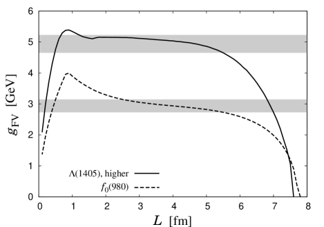
Figure 6: Coupling strength evaluated by Eq. (32) as a function of $L$. The bands show the adopted values of $g_{\rm FV}$ in our study for higher pole of $\Lambda(1405)$ and $f_{0}(980)$.

We next estimate the separation between constituents inside dynamically generated resonances with the procedure developed in Sec. II.1. In our approach, since we expect a downward shift of the real part of the pole position in finite volume for dynamically generated resonances, we firstly identify the real part of the pole position as the mass of the state, and then estimate uncertainties coming from the choice of the mass for the resonances. However, our procedure is valid only when the resonance originates from a bound state. In fact, the poles for $\sigma$, $a_{0}$, and the lower energy pole of $\Lambda(1405)$ do not exhibit the downward mass shift in finite volume. We then conclude that these states are not dominated by the $\bar{K}N$ nor $K\bar{K}$ component, in agreement with the results in Table 3. Therefore, we here consider the properties of the higher pole of $\Lambda(1405)$ and $f_{0}(980)$ resonance with respect to the $\bar{K}N$ and $K\bar{K}$ component, respectively. We first fit the coupling strength $g_{\bar{K}N,\text{FV}}$ ($g_{K\bar{K},\text{FV}}$) to the $L$ dependence of the real part of the pole position of the $\Lambda(1405)$ [$f_{0}(980)$], and then evaluate the mean squared distance between $\bar{K}N$ ($K\bar{K}$) in $\Lambda(1405)$ [$f_{0}(980)$]. As in the case of the bound state, we extract the coupling strength $g_{\rm FV}$ by,

$$g_{\bar{K}N(K\bar{K}),\text{FV}}=\sqrt{\frac{\text{Re}[\tilde{W}_{\rm pole}]-M_{\rm B}}{\displaystyle-\frac{3}{8\pi M_{\rm B}^{2}L}\exp\left[-\bar{\mu}_{\bar{K}N(K\bar{K})}L\right]}},$$ (32)

$$\bar{\mu}_{\bar{K}N(K\bar{K})}=\frac{\sqrt{-\lambda(M_{\rm B}^{2},\,m_{K}^{2},\,m_{N(K)}^{2})}}{2M_{\rm B}},$$ (33)

for higher pole of $\Lambda(1405)$ [$f_{0}(980)$], and for the resonance mass we take $M_{\rm B}=\text{Re}[W_{\rm pole}]$. Here $W_{\rm pole}$ and $\tilde{W}_{\rm pole}$ are resonance pole position in the complex energy plane in infinite and finite volume, respectively. In Fig. 6 we plot $g_{\rm FV}$ in Eq. (32) as a function of the box size $L$. In the figure, we observe rapid change of $g_{\rm FV}$ also in large $L$ region. This is because the pole of the resonance states does not simply move downward in large $L$ region. When $\text{Re}[\tilde{W}_{\rm pole}]=M_{\rm B}$ the coupling strength $g_{\rm FV}$ defined in Eq. (32) vanishes, which takes place at $L\sim 7$–8 fm region in Fig. 6. For $\text{Re}[\tilde{W}_{\rm pole}]>M_{\rm B}$, $g_{\rm FV}$ becomes pure imaginary. Such upward shift of $\Lambda(1405)$ and $f_{0}(980)$ is caused by the repulsion from the lower energy pole [the lower pole of $\Lambda(1405)$ and $\sigma$] in the complex energy plane. For sufficiently small $L$, the downward movement overcomes the repulsion and the mass shift follows Eq. (4). In this case, we observe fairly flat $g_{\rm FV}$ in range $\sim 4\text{ fm}$ both for the higher pole of $\Lambda(1405)$ and $f_{0}(980)$. Hence, as in the bound state case, we adopt $g_{\rm FV}$ in the region where $|dg_{\rm FV}/dL|<\bar{\mu}_{\bar{K}N,K\bar{K}}\text{Re}[W_{\rm pole}]$ is satisfied as the coupling strength from the finite volume effect. The acceptable range is $[1.2\text{ fm},\,5.5\text{ fm}]$ for the higher pole of $\Lambda(1405)$ ($\bar{\mu}_{\bar{K}N}\text{Re}[W_{\rm pole}]=0.53\text{ GeV}/\text{fm}$) and $[2.5\text{ fm},\,5.5\text{ fm}]$ for $f_{0}(980)$ ($\bar{\mu}_{K\bar{K}}\text{Re}[W_{\rm pole}]=0.23\text{ GeV}/\text{fm}$). The adopted values of $g_{\rm FV}$ are shown as bands in Fig. 6 for both $\Lambda(1405)$ and $f_{0}(980)$.

Table 4: Properties of $\Lambda(1405)$ and $f_{0}(980)$ with finite volume effect. Here $\sqrt{\langle r^{2}\rangle}$ is the root mean squared distance between two constituent hadrons, while $\sqrt{\langle R^{2}\rangle}$ is the root mean squared radius evaluated by Eq. (34).

$\Lambda(1405)$, higher pole
$B_{\rm E}=m_{N}+m_{K}-\text{Re}[W_{\rm pole}]$	$8.4\text{ MeV}$
$g_{\bar{K}N,\rm FV}$	$4.6$ – $5.2\text{ GeV}$
$X_{\bar{K}N,\rm{FV}}$	$0.82$ – $1.03$
$\sqrt{\langle r^{2}\rangle_{\bar{K}N,\rm FV}}$	$1.7$ – $1.9\text{ fm}$
$\sqrt{\langle R^{2}\rangle_{\rm size,FV}}$	$1.1$ – $1.2\text{ fm}$

$f_{0}(980)$
$B_{\rm E}=2m_{K}-\text{Re}[W_{\rm pole}]$	$4.2\text{ MeV}$
$g_{K\bar{K},\rm FV}$	$2.7$ – $3.1\text{ GeV}$
$X_{K\bar{K},\rm FV}$	$0.73$ – $0.97$
$\sqrt{\langle r^{2}\rangle_{K\bar{K},\rm FV}}$	$2.6$ – $3.0\text{ fm}$
$\sqrt{\langle R^{2}\rangle_{\rm size,FV}}$	$1.4$ – $1.6\text{ fm}$

The coupling constants and the estimated separations between constituents are summarized in Table 4. As one can see from the table, these resonances are dominated by the $\bar{K}N$ ($K\bar{K}$) component with large spatial extent. In addition, the magnitude of the $\bar{K}N$ ($K\bar{K}$) component $X_{\bar{K}N}$ ($X_{K\bar{K}}$) is in fair agreement with that obtained on the pole position presented in Table 3. Root mean squared distances are $\sqrt{\langle r^{2}\rangle}=1.7$–$1.9\text{ fm}$ for $\Lambda(1405)$ and $2.6$–$3.0\text{ fm}$ for $f_{0}(980)$. Furthermore, we can estimate mean squared radii of the resonance states including the finite size of constituents, $\langle R_{\rm size}^{2}\rangle$, via a relation in Appendix B:

$$\langle R^{2}\rangle_{\rm size}=\frac{m^{2}+m^{\prime 2}}{2(m+m^{\prime})^{2}}\langle r^{2}\rangle+\frac{1}{2}(\langle x^{2}\rangle+\langle x^{\prime 2}\rangle).$$ (34)

with $\langle x^{(\prime)2}\rangle$ being each mean squared radius of the constituents. Because $\langle x^{(\prime)2}\rangle$ is just added with a factor $1/2$ to the mean squared radius of the whole system, size of the constituents always enlarges the mean squared radius of the system. Also, due to the kinematic factor $(m^{2}+m^{\prime 2})/[2(m+m^{\prime})^{2}]$, if masses of two constituents for (quasi-)bound system are very similar to each other, the mean squared distance between constituents $\langle r^{2}\rangle$ corresponds to mean squared diameter rather than radius of the whole system. By using the empirical mean squared radii with respect to the matter distributions for nucleon and kaon estimated from the electromagnetic radii Nakamura:2010zzi ,

$$\langle x^{2}\rangle_{N}\approx 0.7\text{ fm}^{2},\quad\langle x^{2}\rangle_{K,\bar{K}}\approx 0.3\text{ fm}^{2},$$ (35)

the root mean squared radii are evaluated as

$$\sqrt{\langle R^{2}\rangle_{\rm size,FV}}=\begin{cases}1.1\text{ -- }1.2\text{ fm}\quad\text{for }\Lambda(1405),\\ 1.4\text{ -- }1.6\text{ fm}\quad\text{for }f_{0}(980),\end{cases}$$ (36)

to which the contributions from the constituent size are about $0.2\text{ fm}$ and $0.1\text{ fm}$ for $\Lambda(1405)$ and $f_{0}(980)$, respectively. Both the root mean squared distances and radii for $\Lambda(1405)$ and $f_{0}(980)$ are larger than the typical hadronic scale $\lesssim 0.8\text{ fm}$. In this way, the $\Lambda(1405)$ and $f_{0}(980)$ can be interpreted as loosely bound Feshbach resonances.

Now we can compare the present result with previous calculations of the $\bar{K}N$ distance in $\Lambda(1405)$. In Ref. Sekihara:2010uz the complex form factors of $\Lambda(1405)$ was calculated on the pole position in the probe method, and the (real) mean distance between $\bar{K}N$ was evaluated in the bound state approximation. Combining two approaches, we evaluate the complex “mean distance” between $\bar{K}N$ on the pole position at $1426-17i\text{ MeV}$ as

$$\sqrt{\langle r^{2}\rangle_{\bar{K}N}}=1.22-0.63i\text{ fm}\quad|\sqrt{\langle r^{2}\rangle_{\bar{K}N}}|=1.37\text{ fm}.$$ (37)

The mean squared distance of $\bar{K}N$ inside $\Lambda(1405)$ on the pole was also calculated in Ref. Dote:2012bu by using the complex scaling method with an effective coupled-channel potential. The result on the pole at $1419-14i\text{ MeV}$ is

$$\sqrt{\langle r^{2}\rangle_{\bar{K}N}}=1.21-0.49i\text{ fm}\quad|\sqrt{\langle r^{2}\rangle_{\bar{K}N}}|=1.31\text{ fm}.$$ (38)

We find that the estimations of the complex mean distance give a roughly comparable value with the present result, while the precise magnitude is about 30–40 % smaller. In comparison with the real part, the absolute value is slightly closer to our result, but this is not a significant difference. On the other hand, we find that the present method gives consistent values of the root mean squared distance evaluated on the real energy axis. Namely, in Ref. Sekihara:2010uz , the mean distance of the $\bar{K}N$ bound system at 1424 MeV was calculated in the probe method, which leads to

$$\sqrt{\langle r^{2}\rangle}= 1.69\text{ fm}\quad(\text{probe method, $B\sim 11$ MeV}).$$

In Ref. Dote:2008hw , the mean distance was calculated by the effective single-channel potential developed in Ref. Hyodo:2007jq only with its real part, and the results are

$$\sqrt{\langle r^{2}\rangle}= 1.72\text{ -- }1.99\text{ fm}\quad(\text{potential, $B\sim 10$ -- 13 MeV}).$$

This consistency is reasonable, because the box size is defined on the real energy axis in $\tilde{G}(s)$ which is analytically continued to the complex energy plane to probe behavior of resonance states.

Finally let us discuss uncertainties coming from the choice of the mass of the resonance states. Until now we have identified the real part of the pole position as the “mass” of the resonance state, while the resonance mass may have uncertainties of $\pm\Gamma/2=\mp\text{Im}[W_{\rm pole}]$. However, this is a subtle problem, because the mean distance for a bound state is sensitive to the binding energy as seen in Eq. (6). For a weakly bound state, even a small variation of the “mass” (in particular an upward shift) would result in a drastic change of the distance. To assess this uncertainty, we identify $M_{B}=\text{Re}[W_{\rm pole}]-\Gamma/2$, with $\Delta M_{B}$ being unchanged, and calculate the closed channel component $X_{i}$ in addition to the mean distance $\sqrt{\langle r^{2}\rangle_{i}}$. In this case, the compositeness of $\bar{K}N$ and $K\bar{K}$ inside the $\Lambda(1405)$ (higher pole) and $f_{0}(980)$ are about $0.84$ and $0.75$, respectively. The root mean squared distances are calculated as about $1.0\text{ fm}$ for $\Lambda(1405)$ and $1.1\text{ fm}$ for $f_{0}(980)$. We see that the fraction of the closed channel component is obtained within the error band for the result with $M_{\rm B}=\text{Re}[W_{\rm pole}]$. On the other hand, the mean distance for the resonances becomes small, reflecting the increase of the binding energy. This means that the structure of the resonances barely changes with respect to the choice of the “mass”, while the mean distance for the states would decrease when the binding energy is increased. This analysis indicates the importance of the precise determination of the pole position of $\Lambda(1405)$ and $f_{0}(980)$ for the quantitative study of the spatial structure.

IV Conclusion

In this paper the structure of dynamically generated hadrons has been discussed from the viewpoint of the finite volume effect. We have presented a method to extract the properties of a bound state in single-channel scattering using the finite volume mass shift. Introducing a dynamical scattering model, we have shown that the coupling strength, compositeness, and mean squared distance between constituents of the bound state in infinite volume can be reproduced with good accuracy from the mass shift of the bound state in finite volume.

This technique has been extended to a quasi-bound state with finite width in coupled-channel scattering, provided that the width is small. We can estimate the spatial separation of the components in a closed channel from the movement of the pole position along with the finite volume effect on this channel. For an application to physical resonances, we have considered $\Lambda(1405)$, $\sigma$, $f_{0}(980)$, and $a_{0}(980)$ described in chiral unitary approach for coupled-channel hadron scatterings. Applying the finite volume effect on the $\bar{K}N$ and $K\bar{K}$ channels, we have found that the poles for the higher $\Lambda(1405)$ and $f_{0}(980)$ move downward in finite boxes. This result indicates that $\Lambda(1405)$ and $f_{0}(980)$ respectively have large $\bar{K}N$ and $K\bar{K}$ components. Fitting to the mass shift formula, spatial distances of $\bar{K}N$ and $K\bar{K}$ have been evaluated as $1.7$–$1.9\text{ fm}$ and $2.6$–$3.0\text{ fm}$ for higher $\Lambda(1405)$ and $f_{0}(980)$, respectively. Furthermore, with spatial structures of constituents taken into account, the root mean squared radii of $\Lambda(1405)$ and $f_{0}(980)$ are estimated as $1.1$–$1.2\text{ fm}$ and $1.4$–$1.6\text{ fm}$, respectively, to which the contributions from constituent size are about $0.2\text{ fm}$ for $\Lambda(1405)$ and $0.1\text{ fm}$ for $f_{0}(980)$. Both the root mean squared distances and radii for $\Lambda(1405)$ and $f_{0}(980)$ are larger than the typical hadronic scale $\lesssim 0.8\text{ fm}$.

Appendix A Mass shift of bound states in finite boxes

In this Appendix we derive the leading contribution to the mass shift formula for bound states in a periodic finite box of the size $L$, Eq. (4), following Refs. Luscher:1985dn ; Koma:2004wz . Here we consider a bound state with mass $M_{\rm B}$ coupled with a two-particle system with masses $m$ and $m^{\prime}\leq m$. In this Appendix, we work in the Euclidean space. We consider the small binding region as

$$\sqrt{m^{2}+m^{\prime 2}}< M_{\rm B}<m+m^{\prime}.$$ (39)

$\Sigma(P)$	$\tilde{\Sigma}(P)$

Figure 7: Feynman diagrams for the self-energy of the bound state in infinite volume (left) and finite volume (right). The dashed and solid lines denote two distinguishable particles and the double line stands for the bound state. Symbol $L$ in the diagram represents the finite volume effect.

In a finite spatial volume, the momentum of the two-particle system is discretized as $\bm{q}(L)=2\pi\bm{n}/L$ with $\bm{n}\in\mathbb{Z}^{3}$ and the mass of the bound state is shifted to be $\tilde{M}_{\rm B}(L)\neq M_{\rm B}$. Expanding the self-energy in finite volume $\tilde{\Sigma}(P)$ around $P^{0}=iM_{B}$, the mass shift $\Delta M_{\rm B}(L)\equiv\tilde{M}_{\rm B}(L)-M_{\rm B}$ is given by

$$\Delta M_{\rm B}(L)= -\frac{1}{2M_{\rm B}}[\tilde{\Sigma}(P)-\Sigma(P)]+\mathcal{O}(\Delta M_{\rm B}^{2}),$$ (40)

$$P^{\mu}= (iM_{\rm B},\,\bm{0}),$$ (41)

where $\Sigma(P)$ is the self-energy in the infinite volume. While several diagrams contribute to the self-energy Koma:2004wz , the leading effect to the mass shift stems from the diagram shown in Fig. 7. The momentum-discretized loop integral can be expanded in powers of $e^{-iL\bm{m}\cdot\bm{q}}$, $\bm{m}\in\mathbb{Z}^{3}$ with the help of the Poisson summation formula, and the leading contribution can be obtained as

$$\tilde{\Sigma}(P)-\Sigma(P)= \int\frac{d^{4}q}{(2\pi)^{4}}2\sum_{i=1}^{3}\cos(Lq_{i})$$

$$\times\Gamma G_{m}[(1-\delta)P+q]G_{m^{\prime}}(\delta P-q)\Gamma$$

$$+\mathcal{O}(e^{-\sqrt{2}\bar{\mu}L}),$$ (42)

where $\Gamma$ is the three-point vertex function, $G_{m}$ is the propagator with mass $m$, and

$$\bar{\mu}= \frac{\sqrt{-\lambda(M_{B}^{2},m^{2},m^{\prime 2})}}{2M_{B}},$$

with $\lambda(x,\,y,\,z)=x^{2}+y^{2}+z^{2}-2xy-2yz-2zx$.

The momentum fraction $\delta>0$ is chosen to maximize the analytic region of $\text{Im }q_{1}$ as follows. Here we consider that the particles of $M_{B}$ and $m$ have a conserved charge so that we can trace the line which connect the external $M_{B}$ and $m$ propagators of the vertex function $\Gamma$. We then use the same argument with Ref. Koma:2004wz to assign the momenta of the internal lines in the vertex function $\Gamma$. The conditions to avoid singularity are found to be

$$\left(\text{Im}\left\{(1-\delta)P\pm\frac{1}{2}q\right\}\right)^{2} <m^{2}<M_{B}^{2},$$

$$\left(\text{Im}\left\{\delta P\pm\frac{1}{2}q\right\}\right)^{2} <(m^{\prime})^{2}.$$

By choosing

$$\delta=\frac{M_{B}^{2}+(m^{\prime})^{2}-m^{2}}{2M_{B}^{2}},$$

the maximum analytic region for $\text{Im }q_{1}$ is obtained as

$$0\leq(\text{Im }q_{1})^{2}<4\bar{\mu}^{2},$$

The poles of the propagators as functions of $q_{1}$ are given by

$$\bar{q}_{1}= i\sqrt{q_{0}^{2}+q_{\perp}^{2}+\bar{\mu}^{2}+i(2-2\delta)M_{B}q_{0}},$$ (43)

$$\bar{q}_{1}^{\prime}= i\sqrt{q_{0}^{2}+q_{\perp}^{2}+\bar{\mu}^{2}-i2\delta M_{B}q_{0}},$$ (44)

for $G_{m}[(1-\delta)P+q]$ and $G_{m^{\prime}}(\delta P-q)$, respectively. Modifying the integration contour properly, we obtain two terms from these poles with the rest contributions being higher order corrections after the $q_{1}$ integration:

$$\tilde{\Sigma}(P)-\Sigma(P)= I_{1}+I_{1}^{\prime}+\mathcal{O}(e^{-\sqrt{2}\bar{\mu}L}),$$ (45)

with

$$I_{1}= \left.6i\int\frac{dq_{0}d^{2}q_{\perp}}{(2\pi)^{3}}\frac{\exp(iLq_{1})}{2q_{1}}\Gamma G_{m^{\prime}}(\delta P-q)\Gamma\right|_{q_{1}=\bar{q}_{1}},$$

$$I_{1}^{\prime}= \left.6i\int\frac{dq_{0}d^{2}q_{\perp}}{(2\pi)^{3}}\frac{\exp(iLq_{1})}{2q_{1}}\Gamma G_{m}[(1-\delta)P+q]\Gamma\right|_{q_{1}=\bar{q}_{1}^{\prime}},$$

where we have used the rotational invariance. The remaining propagators have a pole in the complex $q_{0}$ plane at

$$\bar{q}_{0}= 0.$$ (46)

The leading contribution to the mass shift formula comes from this pole. To obtain the saddle point expression, we shift the $q_{0}$ integration path from the real axis to $\text{Im }q_{0}=-i(1-\delta)M_{B}$ ($\text{Im }q_{0}=i\delta M_{B}$) in $I_{1}$ ($I_{1}^{\prime}$). The pole contribution from $\bar{q}_{0}$ is picked up by $I_{1}^{\prime}$ term. The leading contribution is then given by

$$I_{1}^{\prime}= 6\int\frac{d^{2}q_{\perp}}{(2\pi)^{3}}\frac{\exp(-L\sqrt{\bar{\mu}^{2}+q_{\perp}})}{2\sqrt{\bar{\mu}^{2}+q_{\perp}}}\frac{g^{2}}{2M_{B}}+\mathcal{O}(e^{-\sqrt{2}\bar{\mu}L}),$$

$$= \frac{3g^{2}}{4\pi LM_{B}}e^{-\bar{\mu}L}+\mathcal{O}(e^{-\sqrt{2}\bar{\mu}L}),$$ (47)

where the coupling constant $g$ is defined as the vertex function $\Gamma$ with all the particles being on the mass shell. In this way, the mass shift formula can be written as

$$\Delta M_{\rm B}(L)= -\frac{3g^{2}}{8\pi LM_{B}^{2}}e^{-\bar{\mu}L}+\mathcal{O}(e^{-\sqrt{2}\bar{\mu}L}).$$ (48)

This formula recovers Eq. (3.37) of Ref. Luscher:1985dn with $m^{\prime}=m$ and with symmetric factor $1/2$ for identical particles.

Note that to obtain positive $\delta$ we need

$$M_{B}^{2}> m^{2}-m^{\prime 2},$$ (49)

which is guaranteed by Eq. (39). All the above argument can be applied to the mass shift of $m$ ($m^{\prime}$) through the $m^{\prime}$-$M_{B}$ loop ($m$-$M_{B}$ loop), by replacing $\{M_{B}\to m,m\to M_{B},m^{\prime}\to m^{\prime}\}$ ($\{M_{B}\to m^{\prime},m\to M_{B},m^{\prime}\to m\}$). However, in the small binding region (39), Eq. (49) is only valid for the self-energy of $M_{B}$, so there is no pole contribution for the self-energies of intermediate particles of $m$ and $m^{\prime}$. The mass shift of the intermediate particles are then given by

$$\Delta m= \mathcal{O}(e^{-m^{\prime}L})$$ (50)

$$\Delta m^{\prime}= \mathcal{O}(e^{-mL})$$ (51)

which do not alter the result (48).

Figure 8: Feynman diagrams for the self-energy induced by the interaction among constituent particles.

Finally we consider how mass shift formula (48) is modified if the constituent particles have their own spatial size. This might be crucial to our discussion on dynamically generated hadronic resonances, because in the real world hadrons have finite spatial size. In the present framework, the size of the constituent particle is induced by the interaction among themselves, which generates the self-energy diagrams shown in Fig. 8. As studied in Ref. Koma:2004wz , the largest contribution to the mass shift is

$$\Delta m= \mathcal{O}(e^{-\bar{\mu}^{\prime}L}),$$

$$\quad\bar{\mu}^{\prime}= m^{\prime}\sqrt{1-\frac{(m^{\prime})^{2}}{4m^{2}}}=\frac{\sqrt{-\lambda(m^{2},\,m^{2},\,m^{\prime 2})}}{2m}.$$

while $\Delta m^{\prime}$ is in higher order than $\Delta m$. Noting that $\sqrt{-\lambda(x^{2},\,m^{2},\,m^{\prime 2})}/2x$ is a monotonically decreasing function of $x$ for $\sqrt{m^{2}-m^{\prime 2}}<x<m+m^{\prime}$, we find $\bar{\mu}<\bar{\mu}^{\prime}$ because of $M_{B}>m$. Again, the mass shift of the constituents is higher order than the leading contribution of Eq. (48). In general, $\bar{\mu}$ represents the virtuality of the intermediate state, and the large mass shift is caused by the channel with small virtuality.

In the applications to physical resonances in Sec. III.2, the finite volume effect is introduced only to the channel of interest, $\bar{K}N$ or $K\bar{K}$. In some sense, we use a box which can be felt only by kaons and nucleons, but not by pions. The spatial structure of hadrons is mainly described by the pionic cloud, which does not cause the mass shift. We therefore conclude that the structure of the constituent hadrons does not alter the mass shift formula in the practical applications to physical resonances. However, the size of the constituent hadrons will modify the “size” of (quasi-)bound states defined by the mean squared radius, as discussed in Appendix B.

Appendix B Relation between size of a bound system and distance of constituents inside the system

In this Appendix we formulate a relation between mean squared radius of a dominantly composite two-body bound system and distance of constituents inside the bound system. First of all we define probability that two constituents inside a bound state are in distance $r$ as $\psi^{2}(r)$ with the normalization,

$$\int d^{3}r\psi^{2}(r)=1.$$ (52)

Here we assume that the function $\psi^{2}(r)$ is spherical, i.e., the two constituents are bound in $s$ wave. This $\psi^{2}(r)$ coincides with the wave function squared with respect to the relative motion of the two-body bound system, and mean squared distance, which we have evaluated in a relation to the finite volume effect, can be evaluated as,

$$\langle r^{2}\rangle=\int d^{3}r\,r^{2}\psi^{2}(r).$$ (53)

Next suppose that two constituents, with masses $m$ and $m^{\prime}$, respectively, have spherical spatial structures of their own. We write the density of their spatial structures as $\rho(x)$ and $\rho^{\prime}(x^{\prime})$, where $x^{(\prime)}$ denotes distance from the center-of-mass of each constituent, with the normalization,

$$\int d^{3}x\rho(x)=\int d^{3}x^{\prime}\rho^{\prime}(x^{\prime})=1.$$ (54)

Their own size can be evaluated as the mean squared radii:

$$\langle x^{2}\rangle_{\rm rad}=\int d^{3}x\,x^{2}\rho(x),\quad\langle x^{\prime 2}\rangle_{\rm rad}=\int d^{3}x^{\prime}\rho^{\prime}(x^{\prime}).$$ (55)

Now we can express how one probes matter distribution of the bound system, in which distance between two constituents is described by $\psi^{2}(r)$ and constituents have their own spatial structures $\rho(x)$ and $\rho^{\prime}(x^{\prime})$. Due to the kinematics, if the relative coordinate of two particles is $\bm{r}$, their positions measured from the center-of-mass of the bound system can be expressed as $m^{\prime}\bm{r}/(m+m^{\prime})$ and $-m\bm{r}/(m+m^{\prime})$, respectively. Therefore, at position $\bm{R}$ measured from the center-of-mass of the bound system, the matter distribution coming from each constituent is expressed as,

$$\sigma(R)=\int d^{3}r\psi^{2}(r)\rho\left(\left|\bm{R}-\frac{m^{\prime}\bm{r}}{m+m^{\prime}}\right|\right),$$ (56)

$$\sigma^{\prime}(R)=\int d^{3}r\psi^{2}(r)\rho^{\prime}\left(\left|\bm{R}+\frac{m\bm{r}}{m+m^{\prime}}\right|\right).$$ (57)

The normalization of $\sigma(R)$ and $\sigma^{\prime}(R)$ are found as,

$$\int d^{3}R\,\sigma(R)=\int d^{3}R\,\sigma^{\prime}(R)=1,$$ (58)

where we have used Eq. (54) to integrate over $R$. In this study we define the whole matter distribution of the bound system as an average of the matter distribution coming from the two constituents as,

$$\text{P}(R)=\frac{1}{2}[\sigma(R)+\sigma^{\prime}(R)],$$ (59)

with a factor $1/2$ for the correct normalization,

$$\int d^{3}R\,\text{P}(R)=1.$$ (60)

Then the mean squared radius of the bound system, $\langle R^{2}\rangle_{\rm size}$, can be evaluated as, after simple integral computations,

$$\langle R^{2}\rangle_{\rm size} =\int d^{3}R\,R^{2}\text{P}(R)$$

$$=\frac{m^{2}+m^{\prime 2}}{2(m+m^{\prime})^{2}}\langle r^{2}\rangle+\frac{1}{2}(\langle x^{2}\rangle_{\rm rad}+\langle x^{\prime 2}\rangle_{\rm rad}).$$ (61)

This gives the relation between distance of constituents inside a bound system and mean squared radius of the whole system. An important feature for the mean squared radius of the system is that each mean squared radius of the constituents is just added with a factor $1/2$. If the size of constituents is zero, $\langle x^{2}\rangle_{\rm rad}=\langle x^{\prime 2}\rangle_{\rm rad}=0$, the mean squared radius of the bound system corresponds to an average of the matter distributions coming from two constituents. The factor $(m^{2}+m^{\prime 2})/[2(m+m^{\prime})^{2}]$ stems from the kinematics. For example, if the constituent masses are same, $m=m^{\prime}$, the factor becomes $1/4$, which means that the mean squared distance between constituents corresponds to, in case that size of constituents is negligible, mean squared diameter rather than radius of the whole system. On the other hand, if one takes $m^{\prime}/m\to 0$ the factor becomes $1/2$, which can be interpreted as that the mean squared radius of the whole system is an average of squared distance $\langle r^{2}\rangle$ coming from the light particle and $0$ from the heavy particle at the origin.

References

- (1) K. Nakamura et al. [Particle Data Group Collaboration], J. Phys. G G 37, 075021 (2010).
- (2) R. H. Dalitz and S. F. Tuan, Annals Phys. 10, 307 (1960).
- (3) R. H. Dalitz, T. C. Wong and G. Rajasekaran, Phys. Rev. 153, 1617 (1967).
- (4) R. L. Jaffe, Phys. Rev. D 15, 267 (1977).
- (5) R. L. Jaffe, Phys. Rev. D 15, 281 (1977).
- (6) J. D. Weinstein and N. Isgur, Phys. Rev. Lett. 48, 659 (1982).
- (7) J. D. Weinstein and N. Isgur, Phys. Rev. D 27, 588 (1983).
- (8) N. Kaiser, P. B. Siegel and W. Weise, Nucl. Phys. A 594, 325 (1995).
- (9) E. Oset and A. Ramos, Nucl. Phys. A 635, 99 (1998).
- (10) J. A. Oller and U. G. Meissner, Phys. Lett. B 500, 263 (2001).
- (11) M. F. M. Lutz and E. E. Kolomeitsev, Nucl. Phys. A 700, 193 (2002).
- (12) T. Hyodo and D. Jido, Prog. Part. Nucl. Phys. 67, 55 (2012).
- (13) A. Dobado and J. R. Pelaez, Phys. Rev. D 47, 4883 (1993).
- (14) J. A. Oller and E. Oset, Nucl. Phys. A 620, 438 (1997) [Erratum-ibid. A 652, 407 (1999)].
- (15) J. A. Oller, E. Oset and J. R. Pelaez, Phys. Rev. D 59, 074001 (1999) [Erratum-ibid. D 60, 099906 (1999)] [Erratum-ibid. D 75, 099903 (2007)].
- (16) T. Sekihara, T. Hyodo and D. Jido, Phys. Lett. B 669, 133 (2008).
- (17) T. Sekihara, T. Hyodo and D. Jido, Phys. Rev. C 83, 055202 (2011).
- (18) M. Luscher, Commun. Math. Phys. 104, 177 (1986).
- (19) S. R. Beane, P. F. Bedaque, A. Parreno and M. J. Savage, Phys. Lett. B 585, 106 (2004).
- (20) Y. Koma and M. Koma, Nucl. Phys. B 713, 575 (2005).
- (21) S. Sasaki and T. Yamazaki, Phys. Rev. D 74, 114507 (2006).
- (22) Z. Davoudi and M. J. Savage, Phys. Rev. D 84, 114502 (2011).
- (23) S. Weinberg, Phys. Rev. 137, B672 (1965).
- (24) D. Lurie and A. J. Macfarlane, Phys. Rev. 136, B816 (1963).
- (25) T. Hyodo, D. Jido and A. Hosaka, Phys. Rev. C 85, 015201 (2012).
- (26) F. Aceti and E. Oset, Phys. Rev. D 86, 014012 (2012).
- (27) M. Luscher, Commun. Math. Phys. 105, 153 (1986).
- (28) M. Doring, U. -G. Meissner, E. Oset and A. Rusetsky, Eur. Phys. J. A 47, 139 (2011).
- (29) A. Martinez Torres, L. R. Dai, C. Koren, D. Jido and E. Oset, Phys. Rev. D 85, 014027 (2012).
- (30) T. Hyodo, D. Jido and A. Hosaka, Phys. Rev. C 78, 025203 (2008).
- (31) Y. Ikeda, T. Hyodo and W. Weise, Phys. Lett. B 706, 63 (2011).
- (32) Y. Ikeda, T. Hyodo and W. Weise, Nucl. Phys. A 881, 98 (2012).
- (33) A. Gomez Nicola and J. R. Pelaez, Phys. Rev. D 65, 054009 (2002).
- (34) E. Oset, A. Ramos and C. Bennhold, Phys. Lett. B 527, 99 (2002) [Erratum-ibid. B 530, 260 (2002)].
- (35) D. Jido, J. A. Oller, E. Oset, A. Ramos and U. G. Meissner, Nucl. Phys. A 725, 181 (2003).
- (36) T. Hyodo and W. Weise, Phys. Rev. C 77, 035204 (2008).
- (37) A. Dote, T. Inoue and T. Myo, arXiv:1207.5279 [nucl-th].
- (38) A. Dote, T. Hyodo and W. Weise, Phys. Rev. C 79, 014003 (2009).