The enrichment history of the intracluster medium: a Bayesian approach

This work measures the evolution of the iron content in galaxy clusters by a rigorous analysis of the data of 130 clusters at $0.1<z<1.3$. This task is made difficult by a) the low signal–to–noise ratio of abundance measurements and the upper limits, b) possible selection effects, c) boundaries in the parameter space, d) non–Gaussian errors, e) the intrinsic variety of the objects studied, and f) abundance systematics. We introduce a Bayesian model to address all these issues at the same time, thus allowing cross–talk (covariance). On simulated data, the Bayesian fit recovers the input enrichment history, unlike in standard analysis. After accounting for a possible dependence on X–ray temperature, for metal abundance systematics, and for the intrinsic variety of studied objects, we found that the present–day metal content is not reached either at high or at low redshifts, but gradually over time: iron abundance increases by a factor 1.5 in the 7 Gyr sampled by the data. Therefore, feedback in metal abundance does not end at high redshift. Evolution is established with a moderate amount of evidence, 19 to 1 odds against faster or slower metal enrichment histories. We quantify, for the first time, the intrinsic spread in metal abundance, $18\pm 3$ %, after correcting for the effect of evolution, X–ray temperature, and metal abundance systematics. Finally, we also present an analytic approximation of the X–ray temperature and metal abundance likelihood functions, which are useful for other regression fitting involving these parameters. The data for the 130 clusters and code used for the stochastic computation are provided with the paper.

1 Introduction

The physics of galaxy clusters is complex because of the interplay of cosmology (structure growth), gas physics, star formation (and its feedback), and possibly AGN. We lack an ab initio theory able to make predictions which are not falsified by data, about how normal baryonic matter collects in dark matter gravitational potential wells and forms galaxies, which in turn influence the intracluster medium (e.g. Young et al. 2011 and references therein). For example, star formation (galaxy feedback) is a suspected source of non–gravitational entropy excess (Buote et al. 2007; Pratt et al. 2006; Sun et al. 2009), yet the amount of star formation required to reproduce the observed X–ray derived quantities (e.g. baryon fraction in gas or mass–temperature scaling relations) is at least ten times greater than the amount of stars observed (Gonzalez et al. 2007; Kravtsov et al. 2009; Andreon 2010).

Owing to the complex behavior of the baryonic matter and the lack of a satisfactory ab initio theory, we can only progress by observational studies of the evolution of the intracluster medium. Measuring the evolution of the gas metallicity is key information for understanding when metals are produced and also at which time the stellar feedback enriches the intracluster medium (e.g. Ettori 2005). Gas metallicity is usually inferred from the fit of the cluster X–ray spectrum, and the derived metal abundance is, largely, the abundance in iron, because data of much higher quality than usually available are needed to constrain the abundance of the other elements.

Determination of the evolution of intracluster medium metal content (Fe, indeed) has been already addressed by previous works, e.g. Balestra et al. (2007), Maughan et al. (2008), Anderson et al. (2009), and Baldi et al (2011), to cite the most recent ones. Key points to be addressed are related to the low–quality determination of most measurements, the possible impact of selection effects, the intrinsic variety of studied objects, the presence of boundaries in the data and parameter space, and metal abundance systematics. Therefore, a proper analysis of the data is mandatory and should be guided by statistical considerations. The main aim of this work is to introduce a statistical approach that can account for all the complex features of the astronomical data and to apply it to available metal abundance measurements.

In Sect. 2 we first convince ourself about the need of revisiting the way abundance analyses are performed. We therefore adopted a Bayesian method (briefly described in Sect. 3, and detailed in Sect. 5) that, when applied to simulated data, is able to recover the input enrichment history. With the new method, we analyse real data (presented in Sect. 4) of 130 clusters observed with Chandra or XMM. Results based on these (real) data are presented in Sect. 6. Sect. 7 describes the advantages of the Bayesian approach and the limitation of their current implementation. Sect. 8 summarises the results. Finally, the Appendix provide the code needed for the revised fitting method.

We adopt $\Omega_{m}=0.3$, $\Omega_{\Lambda}=0.7$, and $H_{0}=70$ km s^-1 Mpc^-1 when computing ages from redshifts.

2 The standard analysis

Iron abundance determination is usually performed using XSPEC (or other X–ray spectral fitting programs). XSPEC (Arnaud 1996) is a code that returns the likelihood $\mathcal{L}$ of the parameters describing the object spectrum, given source and background data, by fitting model spectra of different metallicity and temperature to the data. Users often report a likelihood summary, for example, $Z\,\,^{\Delta^{+}}_{\Delta^{-}}=0.3^{+0.5}_{-0.3}$, where $Z$ is the maximum likelihood (mode) value, and $Z\,+\Delta^{+}$ and $Z\,-\Delta^{-}$ are the points where the likelihood is lower than its maximum by a given factor (e.g. $\Delta\chi^{2}=2\Delta\log\mathcal{L}=1$). XSPEC allows fitting, or freezing, other parameters, such as the cluster redshift, temperature or the Galactic absorption.

When the evolution of the iron abundance is of interest, one should combine measurements of different clusters. Several works (e.g. Balestra et al. 2007, Anderson et al. 2009) combine the information contained in the whole data set in a two step procedure. First, clusters are grouped by redshift. In each redshift bin, all cluster data are fitted simultaneously, with Galactic absorption and redshift fixed at their measured values, both temperatures and metal abundances are free parameters, but temperatures are fitted independently for each cluster, while the metal abundances are tied (i.e. forced to be the same) across clusters. In the second step, the derived iron abundances are fitted vs redshift, and the parameters describing their evolution are found.

To check whether this standard methodology is able to recover the true metal abundance history, we generate simulated data with known input parameters. More precisely, we generate simulated Chandra spectra of the 114 clusters in Maughan et al. (2012), i.e. having the same redshift, temperature, and luminosity as the original clusters and the same exposure time as the original data. Since clusters are well known to have a spread of metal abundance (e.g. De Grandi & Molendi 2001), the individual metal abundance of each cluster is taken to have a scatter around the mean relation $Z_{Fe}/Z_{Fe,\odot}=0.46-0.33z$, taken from Anderson et al. (2009). The adopted amplitude of the scatter, 18%, is derived from the analysis of 130 real cluster data described in following sections. The adopted background and Chandra response matrix are taken from observations (ObsID 10461 and 12003) used in Andreon, Trinchieri & Pizzolato (2011). The generated simulated cluster spectra are then fitted following the standard practice (e.g. Balestra et al. 2007; Maughan et al. 2008) described above. We took the same redshift bins as adopted in Maughan et al. (2008) and Anderson et al. (2009). The derived metal abundance are fitted vs redshift using a $\chi^{2}$ procedure (e.g. Balestra et al. 2007; Anderson et al. 2009) to determine the parameters describing the trend between metal abundance and redshift.

This standard methodology returns as the best–fit relation: $Z_{Fe}/Z_{Fe,\odot}=(0.497\pm 0.015)-(0.463\pm 0.015)z$. It is fairly different in slope from the input relation, $Z_{Fe}/Z_{Fe,\odot}=0.46-0.33z$ because the two slopes differs by $>8\sigma$. Furthermore, the input parameter values are at $\chi^{2}=\chi^{2}_{min}+13$, where $\chi^{2}_{min}$ is the minimum $\chi^{2}$. Other difficulties with the standard analysis are explained in the following sections.

3 The Bayesian approach in a nutshell

Very often we know something about the parameter $\theta$ that we want to study. For example, we may know its order of magnitude. This knowledge may be crystallised in a mathematical expression, $p(\theta)$, stating that, for example, some values are more probable than others according to a specific expression $p(\theta)$ (e.g. $p(\theta)\propto e^{-\theta}$). This probability distribution is called the prior. Observations return a value, $obs\theta$ and an error, or, to be more precise, how likely observing $obs\theta$ is when the true value is $\theta$, $p(obs\theta|\theta)$. This probability distribution is named the likelihood, i.e. a measure of how variable the output $obs\theta$ is when the input value is $\theta$. The likelihood (“instrument calibration”) is certainly interesting, but we may perhaps want to know which values of $\theta$ are more probable after having observed $obs\theta$, i.e. to derive the probability of $\theta$ given $obs\theta$, $p(\theta|obs\theta)$. The Bayes theorem tell us that to obtain the latter, called the posterior probability distribution, we need to multiply the prior and the likelihood (times a constant of no interest in parameter estimation). For a deeper understanding of Bayesian methods, one may consult, for example, Gelman et al. (2003), and for astronomical introductions, Trotta (2007), Andreon & Hurn (2010, 2011), and Andreon (2010b, 2012), among others.

In this work, we adopt this Bayesian approach. When applied to the simulated data above, it returns $Z_{Fe}/Z_{Fe,\odot}=0.45\pm 0.02-(0.31\pm 0.04)z$, well within $1\sigma$ from the input trend. As detailed below, it improves upon previous analysis because it operates correctly on likelihoods. We therefore adopt it for analysing the real data of 130 clusters, as described in the following sections in detail.

Readers not interested in the fitting details may skip Sects. 4 and 5, where we account for non–independent and non–Gaussian data, for the existence of an intrinsic diversity in metal abundances, for mass–dependent selection effects, and for systematic differences between Chandra- and XMM- derived metal abundances.

Figure 1: Old and new Chandra values of metal abundance for the quartile with the smallest percentage errors on metal abundance. The line indicates the one–to–one relation.

4 The cluster sample & the new metal abundance measurements

Our sample is composed of two subsamples: 114 galaxy clusters at $0.1<z<1.2$ observed with Chandra ACIS-I (Maughan et al. 2008) and 29 galaxy clusters at $0.3<z<1.3$ observed with XMM (Anderson et al. 2009). For consistency with the Anderson et al (2009) analysis, the central region of the clusters is not excised in Chandra measurements.

The samples we studied, as well as the two starting lists, are heterogeneous collections without any known selection function being basically, what is available in the Chandra and XMM archives. The lack of a known selection function is the major limitation of current samples with available metal abundance measurements, hence also of our work, although we control for mass–dependent selection effects, as described in Sect. 5.4.

Maughan et al. (2008) present metal abundance and temperature values for his sample using the CALDB version 3.2.3. The data have been reprocessed (Maughan et al. 2012) with the up–to–date Chandra calibration, mainly improving the Chandra mirror effective area and the ACIS contamination model. In the current work we also revisit the XSPEC settings appropriate for metal abundance determination (Sect. 5.7). These newly derived metal abundances are used here and are listed in Table 1.

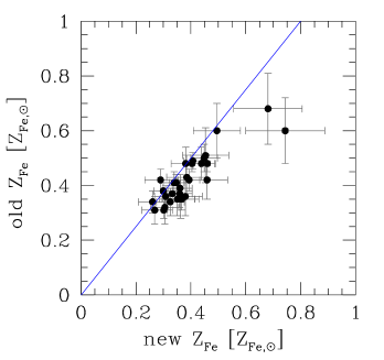
Figure 1 compares old and new Chandra metal abundances for the quartile with the smallest percentage error on metal abundance (to limit crowding). From the analysis of the whole sample, we found that metal abundances derived with up–to–date calibrations tend to be $12\pm 3$ % larger than old values. A $\chi^{2}$ analysis returns no evidence of a redshift–dependent correction, with a 68 % confidence interval of $[-0.06,0.03]$ on the the redshift–dependent term.

Fe abundances are normalised to solar abundances in Anders & Grevesse (1989). In particular, the solar abundance of iron atoms relative to hydrogen is $4.68\ 10^{-5}$.

5 The fitted model

As emphasised by the simulation in Sect. 2, the key ingredient for a trustful determination of the Fe abundance history with current data lays in the statistical aspect of the analysis, and this guides our presentation.

5.1 Duplicate clusters

Thirteen clusters appear in both the Maughan et al. (2012) and Anderson et al. (2009) lists, which make the data dependent. The lack of independence is quite dangerous if not accounted for, for example, if one computes the width (intrinsic scatter, dispersion) or the mean of a distribution (of abundances, for example) in which some elements are listed twice.

We want independent data and, at the same time, want to make full use of the available information. Therefore, we remove duplicates from the list of fitted data (specifically, we keep the data set that provides smaller errors on metal abundances), and use the removed data in Sect. 5.5 to derive the prior on metal abundance systematic.

The problem of duplicate clusters has already occurred in previous analysis (e.g. Anderson et al. 2009, Balestra et al. 2007), but is first addressed here as far as we are aware.

5.2 Enrichment history

Metal abundance, $Z_{Fe}$, must be positive at all redshifts. Some authors (e.g. Anderson et al. 2009) choose to fit the evolution of the metal abundance with a linear relation, which may lead to unphysical results. For example, the best–fit in Anderson et al. (2009) crosses $Z_{Fe}=0$ at $z\sim 1.2$ i.e. within the range of the data analysed by them. This is clearly unphysical, also considering that clusters at higher redshift exist (e.g. Stanford et al. 2005, 2009; Andreon et al. 2009, etc.), and for these the best–fit relation predicts negative metal abundances. We chose to fit metal abundance measurements by a function that can never cross the physical boundary $Z_{Fe}=0$. It is also plausible that the Fe abundance was zero at the time of the Big Bang. Therefore, we adopted an exponential function for the enrichment history parametrised as

$$f(t_{i})=\frac{Z_{Fe,z=0.2}}{1-e^{-11/\tau}}(1-e^{-t_{i}/\tau})$$ (1)

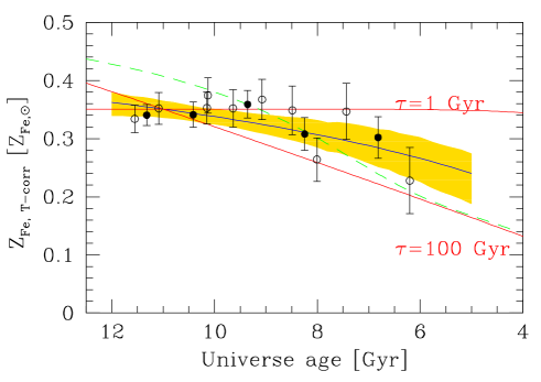
where $\tau$ is the characteristic time (in Gyr) and $t_{i}$ is the Universe age (in Gyr) at the redshift of the $i^{th}$ cluster. The denominator in Eq. 1 was chosen to have $Z_{Fe,z=0.2}$ as second parameter, i.e. the Fe abundance (in solar units) at $z=0.2$, a redshift sampled well by the data used. This choice simplifies the interpretation of the results. The $\tau$ parameter regulates when enrichment occurs: early in the Universe history (small $\tau$’s) or gradually over time (large $\tau$’s). Two extreme enrichment histories are depicted in the right hand panel in Fig. 4. Our choice of using an exponential function to describe the evolution of the metal abundance is mathematically equivalent to assuming a linear function on the log of the metal abundance: $Z\propto e^{-t/\tau}\equiv\log Z\propto-t/\tau$.

With this model, metal abundance is always positive. Our modelling of the Fe enrichment assumes that the enrichment starts at the Big Bang. While one may argue that enrichment starts at a later age, this is irrelevant for our modelling as long as the data do not sample very early enrichment phases (i.e. $t\ll 4$ Gyr, or $z\gg 1.5$). In the future, when observations will reach the epoch of first enrichment, we will need to replace Eq. 1 with a more complex formula, for example one with two characteristic times to account for an initial enrichment by core collapse supernovae followed by a metal production spread on longer time scales. This operation is very easy to implement, as detailed in the Appendix.

5.3 Intrinsic scatter

Galaxy clusters show a spread of Fe abundance at the very least because cool–core and not cool–core clusters have different metallicities (De Grandi & Molendi 2001). The scatter may also be due to chemical inhomogeneities and abundance gradients within clusters, differences in cluster star formation histories, differences in cluster metallicities (which affect the chemical enrichment in as much as the chemical “yields” depend on metallicity e.g. Woosley & Weaver 1995), different ages of the stellar populations in clusters, and different cluster masses. Independently of the physical source of the spread, the presence of an intrinsic scatter implies that the information content of a single measurement is lower than indicated by the error, especially when the latter is comparable to, or is smaller than, the intrinsic scatter. The intrinsic scatter acts as a floor: the information content of a measurement is not better than the intrinsic scatter, no matter how precise the measurement is. Therefore, above some signal–to–noise ratio, the information content of a single measurement no longer increase; in other words, two measurements with error $\sigma$ smaller than, or comparable to, the intrinsic scatter are better than one with error $\sigma/\sqrt{2}$. Therefore, in the presence of intrinsic scatter, measurements cannot be combined using errors as weight: the error derived from the simultaneous fit (as in the standard analysis) will be underestimated because it ignores the metal abundance spread. Furthermore, the task of simultaneously fitting spectra becomes prohibitive if the intrinsic scatter is not known a priori because the weight to be used is unknown, exactly as in Fe abundance measurements. Furthermore, unless individual spectra all have the same S/N, the best–fit metal abundance will be biased toward the metal abundance of the spectrum with the highest S/N. Finally, if an intrinsic scatter is not allowed, a redshift trend may be overly driven by a single high S/N measurement, as noted by Baldi et al. (2011), who note the dramatic effect of including, or removing, a very low upper limit in a fit where the intrinsic scatter is not allowed.

Instead of fitting spectra of clusters with a single value of Fe abundance forced to be the same across clusters, as in the standard analysis, we do a simultaneous analysis of all the individual spectra allowing Fe abundances to differ from cluster to cluster and inferring the intrinsic scatter at the same time. Because metal abundance may evolve and has a possible temperature dependence, the intrinsic scatter should be fitted at the same time as other parameters. We model the distribution of Fe abundances as a log–normal process of unknown intrinsic scatter,

$$Z_{Fe,i}\sim log\mathcal{N}(lnf(t_{i}),\sigma^{2}_{intr})\quad.$$ (2)

Expressed in words, the Fe abundance of the $i^{th}$ clusters, $Z_{Fe,i}$ shows a log–normal intrinsic scatter $\sigma_{intr}$, around the median value, $f(t_{i})$. Of course, a Gaussian scatter in $Z_{Fe,i}$ is precluded by the positive nature of the Fe abundance. The tilde symbol reads “is distributed as” throughout.

Our adoption of a log–normal scatter removes the major limitation of previous analysis, namely the tension between data (that require a spread) and the adopted fitting model (that assumes a unique metal abundance value at a given redshift). The statistical name for this tension is misspecification, and we quantify its amplitude in Sect. 6.2. The choice of a log–normal scatter in $Z_{Fe}$, i.e. a Gaussian scatter in $\log Z_{Fe}$, is motivated by its being the simplest solution to break the previously adopted assumption of no scatter. With data of adequate quality, the shape of the distribution itself may be inferred from the data; however, this is precluded by the current samples. In Sect. 7.3 we test our log–normal assumption by adopting instead a Student’s $t$ distribution.

5.4 Controlling for temperature

The Fe abundance might depend on cluster mass (e.g. Balestra et al. 2007; Baumgartner et al. 2005). If neglected, this dependence induces a bias in determining the evolution of the Fe abundance unless the studied sample is a random, redshift–independent sampling of the cluster mass function. For example, if the average mass of clusters in the sample increases with redshift and the Fe abundance increases with temperature $T$, one may observe a spurious Fe abundance tilt (increase) with redshift. Other combinations of dependences are potential sources of a bias, such as a decreasing metal abundance with increasing $T$. Among these combinations, we should also consider those that include variations in the mass range sampled at a given redshift (e.g. lower redshifts sampling a wider cluster mass range). To summarise, given the uncontrolled nature of the available samples, one must at the very least control for $T$ (i.e. a mass proxy) in order to avoid the risk of mistaking a mass dependency for an Fe abundance evolution. Even if data are unable to unambigously determine a $T$ trend, controlling for $T$ allows a trend to be there as much as allowed by the data and not to overstate the statistical significance of a redshift trend.

We control for mass by allowing the Fe abundance, $Z_{Fe}$, to depend on $T$. We adopt a power law relation, following Balestra et al. (2007), between metal abundance and temperature, $Z_{Fe}\propto T^{\alpha}$. Since clusters are at different redshifts, and $Z_{Fe}$ is possibly evolving, we need to fit both the $T$ dependency and evolution at the same time.

Figure 2: Determination of the shape of the likelihood function of temperature. Measured values (points) and expectations for a normal (red solid line) and a log–normal (green curve) likelihood.

5.5 Metal abundances systematics

Metal abundances may show some systematic differences when derived by two different teams using data taken with two different X–ray telescopes (Chandra and XMM) analysed with similar, but not identical, procedures. In particular, based on 13 common clusters, XMM abundances (derived by Anderson et al. 2009) are $0.77\pm 0.065$ times those measured (by us) with Chandra.

We account for this systematics by allowing metal abundances measured by different telescopes to differ by a multiplicative factor as large as allowed by the data. Observationally, the factor is constrained by measurements of both telescopes having to agree after the multiplicative scaling. Of course, to not mistake systematics with differences due to the intrinsic scatter or evolution, dependence on all three parameters have to be accounted for. Therefore, systematics have to be inferred at the same time as the other parameters. Expressed mathematically, we only need to introduce a quantity, $tid$, that takes the value of zero for the Chandra data, and one for the XMM data (a convention, but one may choose to do the reverse), and multiply metal abundances by the factor, $1+fact*tid$, to bring all measurements on a common scale (Chandra, with our convention):

$$Z_{Fe,i,cor}=Z_{Fe,i}*(1+fact*tid_{i})*T^{\alpha}\quad.$$ (3)

The $T^{\alpha}$ term is there to control for $T$, i.e. to account for a possible dependence of the Fe abundance on $T$ (Sect. 5.4).

5.6 Temperature likelihood

X–ray temperature errors are often asymmetric; i.e., temperatures are usually quoted in the form $modeT^{+\Delta^{+}}_{-\Delta^{-}}$, with $\Delta^{+}\neq\Delta^{-}$. As mentioned in the introduction, $\Delta^{\pm}$ are the points where the likelihood is lower than its maximum by a given factor (see Avni 1976, Press et al. 1986, or the Sherpa or XSPEC manual for the numerical values to be used). A Gaussian function is, of course, symmetric. Therefore, the temperature likelihood cannot be a Gaussian. We adopt the symbol $modeT$ to emphasise that the quoted value is the maximum likelihood value (i.e. the mode). A plot of the temperature likelihood of clusters (e.g. Fig. 12 in Andreon et al. 2009) reveals the likelihood asymmetry and suggests that it can be described with a log–normal shape. The log–normal distribution has the welcome property of being bounded in the positive part of the real axis, i.e. avoids negative $T$.

Our suggestion of a log–normal temperature likelihood can be tested with our large sample. Figure 2 shows $\Delta^{+}/modeT$ vs $\Delta^{-}/modeT$. For a log–normal function, the points should follow the curved (green) line. If the likelihood were Gaussian, the locus (straight line) $\Delta^{+}/modeT=\Delta^{-}/modeT$ should be followed. Figure 2 shows that the log–normal likelihood captures the data behaviour. Simple algebra, together with the knowledge of the definition of $\Delta^{+}$ and $\Delta^{-}$ (see XSPEC or Sherpa manuals), allows us to analytically compute the likelihood parameters. For a log–normal model with location $\mu$ and scale $\sigma$, we find

$$\sigma_{\pm}=\pm\ln(modeT\pm\Delta^{\pm})\mp\ln(modeT)\quad.$$

Using real data, $\sigma_{+}$ and $\sigma_{-}$ slightly differ because every measurement, including $\Delta^{\pm}$ values, is subject to errors and rounding. We thus take the average of $\sigma_{\pm}$ as the value of $\sigma_{T,i}$.

To sum up, the whole section may be summarised by the mathematical expression:

$$modeT_{i}\sim log\mathcal{N}(\ln T_{i},\sigma^{2}_{T,i})\quad,$$ (4)

which allows us to account for asymmetric temperature errors. While our statement of the non–normal $T$ likelihood is certainly not new, to our knowledge this is the first time the non–normal $T$ likelihood has been implemented in a regression fitting involving $T$.

Figure 3: Abundance likelihood function of four clusters, chosen to illustrate the likelihood shape in various cases. The open circles show the likelihoods derived with XSPEC, whereas the solid curves present a Gaussian approximation of them.

5.7 Fe abundance likelihood

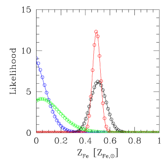
Inspection of plots of the metal abundance likelihood (four examples are shown in Fig. 3, computed using XSPEC) shows, in agreement with Leccardi & Molendi (2008), that the metal abundance likelihood has a Gaussian shape. In formulae

$$modeZ_{Fe,i}\sim\mathcal{N}(Z_{Fe,i,cor},\sigma^{2}_{Z_{Fe,i}})\quad.$$ (5)

This implies that a negative $modeZ_{Fe,i}$ can be found, most often for low S/N measurements.

The parameters of the equation above are determined by fitting the data with XSPEC. We emphasise, however, that the input numbers of this equation, $\sigma_{Z_{Fe,i}}$ and $modeZ_{Fe,i}$, are not, generally speaking, the standard XSPEC output numbers because XSPEC uses different definitions of the likelihood location and width.

The mode of the likelihood on the unrestricted range $Z_{Fe}\in[-\infty,\infty]$ is $modeZ_{Fe,i}$. We accept negative $modeZ_{Fe,i}$ values as a way to describe the likelihood wing at $Z_{Fe,i}>0$ when the latter shows no maximum there (e.g. the leftmost likelihood in Fig. 3). Negative $modeZ_{Fe,i}$ indicate that the measurement has such a low S/N that the likelihood has no peak in the physical range ($Z_{Fe,i}>0$), and the data only offer an upper limit to the cluster metal abundance. We emphasise that in the Bayesian approach inferences come from the posterior, not from the likelihood alone. Since the abundance posterior distribution is only non–zero for $Z_{Fe}>0$ (because of the prior, Eq. 6) every point estimate of the cluster abundance (e.g. posterior mean, median) is always positively defined, as good sense requires, even when $modeZ_{Fe,i}<0$. XSPEC’s $maxZ_{Fe,i}$ is the mode of the likelihood in a restricted range (set at $Z_{Fe}\geq 0$ by default). It differs from $modeZ_{Fe,i}$ when the likelihood has no peak at $Z_{Fe,i}>0$ (e.g. the left–most likelihood in Fig. 3).

The usual width of the Gaussian is $\sigma_{Z_{Fe,i}}$. For the author’s opinion, it is the most straightforward estimate of the metallicity uncertainty. XSPEC instead quantifies the likelihood width by $\Delta^{\pm}$ values, determined by the points where the likelihood is lower than its maximum by a given factor. If the peak is far away from the zero boundary (mathematically: if $modeZ_{Fe,i}-\sigma_{Z_{Fe,i}}>0$), as in the two rightmost likelihoods in Fig. 3, the two estimates of the likelihood width coincide. However, these estimates may differ widely, as in the left–most likelihood in Fig. 3, where $modeZ_{Fe,i}+\sigma_{Z_{Fe,i}}\approx 0$. In such cases, $\Delta^{+}$ value is low, but the error $\sigma_{Z_{Fe,i}}$ is large (the data only offer an upper limit to the cluster metal abundance.) Therefore, one should not overlook the difference between $\Delta^{\pm}$ and $\sigma_{Z_{Fe,i}}$. If $modeZ_{Fe,i}-\sigma_{Z_{Fe,i}}<0$, then $\Delta^{-}$ differs from $\Delta^{+}$, even for a Gaussian likelihood (e.g. for the two leftmost likelihoods displayed in Fig. 3). This situation is quite usual for cluster metal abundances, and in fact asymmetric $\Delta^{\pm}$ values are often quoted (e.g. $0.3^{+0.5}_{-0.3}$).

The two definition sets may be made identical by removing the XSPEC default positivity constraint to abundances. Alternatively, one may note that $\sigma_{Z_{Fe,i}}=\Delta^{+}$, except when $maxAb=0$. We adopted this property for Anderson et al. (2009) abundance measurements. When XSPEC (with the positivity constrain set on) instead returns $maxAb=0$ (e.g. CLJ0522-3625), the XSPEC positivity constraint has to be removed, and we accept negative $modeZ_{Fe,i}$ values. This choice allows us to analyse samples, like the studied one that include both upper limits and precisely determined values. In this way, including upper limits is automatically accounted for in our determination of the metal abundance history.

We verified that if one overlooks the difference between $\Delta^{\pm}$ and $\sigma_{Z_{Fe,i}}$, the trend between metal abundance and redshift is tilted because these noisy values occur only at high redshift.

Table 1 lists the cluster ID, the redshift $z$, the temperature $modeT_{i}$, and its $\sigma_{T,i}$, the metal abundance $modeA_{i}$ and its $\sigma_{Z_{Fe,i}}$, and indicates whether the data comes from Chandra or XMM ($tid$). The table has 130 lines in its electronic version. About 70% of the listed temperature or metal abundance values and errors have been newly derived (the remaining values are taken from Maughan et al 2012 or Anderson et al. 2009). We emphasise, as explained above, that negative values for $modeZ_{Fe}$ in Table 1 are correct (whereas every posterior estimate of $Z_{Fe}$ is positive) and are meant to describe the Gaussian likelihood wing at $Z_{Fe,i}>0$. Forcing them to be positive would spuriously bend the trend between metal abundance and redshift.

Figure 4: Metal abundance, on the Chandra scale, vs Universe age. Left Panel: Observed values of metal abundance and errors are corrected for the $T$ dependence and for the Chandra vs XMM systematic as determined by a simultaneous fit of all parameters. Red (blue) circles refer to Chandra (XMM) measurements. Points indicate the maximum a posteriori, whereas error bars represent the shortest 68% probability intervals. The solid line marks the mean fitted relation between metal abundance and redshift, while the dashed line shows this mean plus or minus the intrinsic scatter $\sigma_{scat}$. The shaded region marks the 68% highest posterior credible interval for the regression. The distances between the data and the mean model are due in part to the measurement error and in part to the intrinsic scatter. Right Panel: Solid points are metal abundances, corrected as in the left panel, but binning in 5 (solid points) or 10 (open points) redshift bins. The solid line and shading are as in the left panel. Two extreme enrichment histories (red lines) and the Ettori (2005) model (green dashed line) are also plotted .

5.8 Priors

At this point, we have the data and we described the mathematical link between the quantities that matter for our problem (Eqs. 1 to 5). To complete the analysis, we now specify what else we know about the parameters. Except for metal abundance systematics, we assume we know very little about the parameters; i.e., we adopt for all quantities priors wide enough to certainly include the true value, but not so wide to include unphysical values. For the systematics on metal abundance we adopt as prior the result of our metal abundance comparison (Sect. 5.5) for the 13 clusters in common between Chandra and XMM lists: $0.77\pm 0.065$.

Table 1: Id, Redshift, metal abundances, temperatures, and their $\sigma$ values, and data source (zero for Chandra, one for XMM–Newton).

id	$z_{i}$	$modeZ_{Fe,i}$	$\sigma_{Z_{Fe,i}}$	$modeT_{i}$	$\sigma_{T,i}$	$tid_{i}$
		[$Z_{Fe,\odot}$]	[$Z_{Fe,\odot}$]	[keV]
MS1008.1-1224	0.301	0.41	0.11	5.00	0.06	0
CLJ1113.1-2615	0.725	0.51	0.41	3.80	0.18	0
RXJ1716.9+6708	0.813	0.55	0.22	6.30	0.14	0
A2111	0.229	0.23	0.13	6.40	0.09	0
A697	0.282	0.38	0.07	9.80	0.05	0

This table has 130 lines in its electronic version.

Specifically, the prior of the mean Fe abundance at $z=0.2$, $Z_{Fe,z=0.2}$ is taken as uniform between 0 and 1 $Z_{Fe,\odot}$; i.e., the mean Fe abundance may take any value in this wide range with no preferred value. Similarly, for the true value of the cluster temperature, we took an uniform distribution over a wide range 1 to 20 keV, which generously includes all plausible values for the true temperature of the studied clusters. Their observed values range from $2.4$ to $14.7$ keV. Similarly, the prior of the intrinsic scatter of Fe abundance, $\sigma_{intr}$ is also taken as uniform between 0 and 1, a range wide enough to certainly include the true value. The prior on $\tau$ is taken to be uniform between the wide range 1 and 100 Gyr. More extreme values give enrichment histories that are indistinguishable from $\tau=1$ Gyr or $\tau=100$ Gyr in the redshift range explored in this work. This is the reason we adopted these values as boundaries of the explored parameter space. If $\tau\approx 1$ Gyr, the Fe abundance is constant (see right panel of Fig. 4) and if $\tau\approx 100$ Gyr, models change almost linearly (see right panel of Fig. 4) with age. The prior of the power–law dependency of iron abundance on temperature is a Student’s $t$ (uniform on the angle $a=\arctan\alpha$), as in previous works dealing with a slope computation (e.g. Andreon et al. 2006, Andreon & Hurn 2010). In formulae the priors are

$$Z_{Fe,z=0.2} \sim \mathcal{U}(0,1)$$ (6)

$$\tau \sim \mathcal{U}(1,100)$$ (7)

$$\alpha \sim t_{1}$$ (8)

$$fact \sim \mathcal{N}(0.77-1,0.065^{2})I(-1,)$$ (9)

$$\sigma_{intr} \sim \mathcal{U}(0,1)$$ (10)

$$T_{i} \sim \mathcal{U}(1,20)$$ (11)

where the $I(-1,)$ operator truncates the likelihood at $-1$, to avoid $(1+fact)$ taking negative (unphysical) values.

How much our conclusions depends on the chosen priors is detailed below, but we can anticipate that the dependence is almost zero.

Figure 5: Probability distribution for the parameters of the metal abundance vs redshift fit. The solid circles show the posterior probability distribution as computed by MCMC, marginalised over the other parameters. The red curve (when present) shows a Gauss approximation of it. The dashed curve displays the adopted prior. The shaded (yellow) range shows the 95% highest posterior credible interval.

5.9 Stochastic computation

At this point, we have the data in the right format (i.e. with $\sigma$’s), we have the description of the link between interesting parameters (Eqs. 1 to 5), and we have specified what we know about the parameters before seeing the data (Eqs. 6 to 11). We now need to use the Bayes theorem and to compute the posterior probability distribution of the parameters. Just Another Gibb Sampler (JAGS) can return it in form of (Markov Chain) Monte Carlo samplings. From the Monte Carlo sampling one may directly derive mean values, standard deviations, and confidence regions of any parameter or any parameter–depending quantity. For example, for a 90 % interval on $\tau$, it is sufficient to take the interval that contain 90 % of the $\tau$ samplings.

Readers who are less familiar with Bayesian methods may just think that we use JAGS to correctly combine likelihoods (data) in order to extract parameters values. The JAGS code is given in Appendix.

6 Results

6.1 Parameter estimation

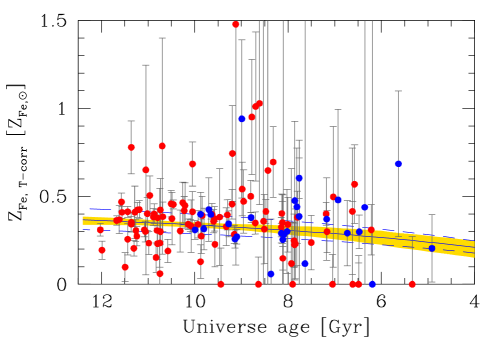
The result of the fit of metal abundance and temperature values for the sample of 130 clusters is summarised in Figs. 4 and 5. The left–hand panel of Fig. 4 shows the data, corrected for the $T$ dependence and for the metal abundance systematics, as determined by a simultaneous fit of all parameters, the mean fitted relation between metal abundance and Universe age, this mean plus or minus the intrinsic scatter $\sigma_{scat}$, that turns out to be $0.18\pm 0.03$, i.e. 18 % of the Fe abundance value, and the 68% highest posterior credible interval of the fit.

An useful approximation of the mean trend is given by

$$\frac{0.35}{1-e^{-11/6}}(1-e^{-t/6})\quad,$$ (12)

with errors given by $\pm 0.02$ at ages greater than 7 Gyr, and $\pm 0.04$ at younger ages.

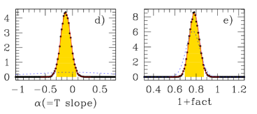
Figure 5 shows prior and posterior probability distributions of the parameters. The figure highlights two key points: first, the posterior distribution of all parameters is much more concentrated than the prior; i.e., data are highly informative about these parameters. As a consequence, conclusions on these parameters do not depend on the adopted prior (see below for discussion about panel e). Second, the posterior probability distribution of all parameters except $\tau$ is described well by a Gaussian distribution.

The metal abundance at $z=0.2$, $Z_{Fe,z=0.2}$ is fairly well determined: $0.35\pm 0.01$ $Z_{Fe,\odot}$ (Fig. 5, panel a). The intrinsic scatter in abundance values, after controlling for $T$, taking evolution and systematics into account, is $0.18\pm 0.03$ (Fig. 5, panel c). The posterior distribution of the e–folding time $\tau$ avoids both low (near 1 Gyr) and high (above 20 Gyr) values and peaks on timescales of 4-6 Gyr. The (highest posterior) 68 % probability interval is [1.4-8.6] Gyr. The flat shape of the right tail of the posterior occurs because models with $\tau\approx 20$ Gyr show very tiny differences, too small to be measurable with the current sample. The key point to keep in mind is that the posterior probability distribution peaks at $\tau\approx 4-6$ Gyr; i.e., enrichment histories completed at high redshift or delayed at late times are not favored by the data, a statement that we further quantify in Sect. 6.2. While entropy feedback predates cluster formation (Ponman et al. 1999), metal abundance enrichment is not exhausted at high redshift. We emphasise that if metal abundance upper limits were incorrectly dealt with (and everything else dealt correctly), shorter e–folding time $\tau$ (more strongly evolving metal abundance histories) would be found with increased (spurious) statistical significance.

The slope $\alpha$ of the metal abundance vs temperature scaling is certainly not steep, but, apart from that, is poorly determined: $-0.12\pm 0.09$ (Fig. 5, panel d). As mentioned, by letting it be as large as permitted by the data allows us not to mistake a $T$ dependency, joined to a non–random sample selection, with a metal abundance evolution. It also allows us to remove a source of concern, because we now know that mass–selected effects are minimal, if there are any, for cluster samples similar (in cardinality, mass, and redshift range) to our one. The slope found by Balestra et al. (2007), $-0.47$ is $\sim 3.8\sigma$ away from our determination, but it has been derived using a three times smaller sample ignoring the evolution of the iron abundance, the intrinsic scatter, and metal abundance systematics.

Metal abundances measured with XMM turn out to be $0.78\pm 0.045$ times those measured with Chandra (Fig. 5, panel e), in agreement with (and improving upon) our estimate of Sect. 5.5 (prior), $0.77\pm 0.065$. If an uniform prior were adopted for this parameter, the posterior mean would be $0.80\pm 0.07$. The agreement between the amplitude of the systematic derived from the 130 clusters alone ($0.80\pm 0.07$) and the one independently derived from the 13 clusters observed by both Chandra and XMM ($0.77\pm 0.065$) indicates that the measurement of the abundance systematics is robustly determined. The precision achieved by comparing the metal abundance of 13 clusters with both XMM and Chandra measurements ($0.065$) is similar to the one inferred from a ten times larger sample that assumes no metallicity bias between clusters observed by Chandra and by XMM ($0.07$).

The overall decline in the metal abundance that we observe, also reported in the right–hand panel of Fig. 4, is slower than in the phenomenological model of Ettori et al. (2005). The offset at low redshift between Ettori et al. (2005) and current metal abundance measurements is due to the change of the Chandra calibration. In fact, by repeating our analysis using the older metal abundances (from Maughan et al. 2008), we found better agreement at low redshift with the Ettori et al. (2005) model.

Figure 6: Illustration of how the fitted data reject the best–fit in previous works. The bottom–left panel shows the $\chi^{2}$ of the individual data points (from Balestra et al. 2007, chosen for illustration) vs redshift. The $\chi^{2}$ is computed using the Balestra et al. (2007) best–fit. The top left-hand panel shows the same, but for data extracted from a realisation of the Balestra et al. (2007) fitted model. Real data scatter much more than simulated data, as quantified in the top right-hand panel: the total $\chi^{2}$ of 30000 realisations of the Balestra et al. (2007) model is histogrammed, together with the total $\chi^{2}$ of their sample (vertical line). Either using $\chi^{2}$ tables (or the usual rule $\chi^{2}/\nu$, $\nu\approx 54$) or more sophisticated simulations, the Balestra et al. (2007) data reject their best–fit at $>99.9$ confidence.

Because of the youthfulness of theoretical (numerical or analytic) models (see Fabjan et al. 2008 for a careful report about the limitations of their own numerical modelling), our observational constraints on the metal abundance history cannot be transformed in physical constraints on cluster parameters, so we cannot interpret the observational results as due to clumps of enriched gas falling in the cluster centre (e.g. Cora et al. 2008), a recent pollution by metals previously present in stars (e.g. Calura et al. 2007), an enhanced star formation at low redshift, or any other proposed mechanisms. There are two reasons that prevent us from drawing firm conclusions: first, different physical mechanisms implemented in models are able reproduce this specific cluster observable, the metal abundance history, and second, these models are generally not able to reproduce other related observables (e.g. the $L_{X}-T$ scaling relation, the stellar baryon fraction, the temperature profile, etc.). For example, numerical simulations produce the right amount of metals, but generate ten times too many stars (Andreon 2010).

6.2 Model missfit and evidence for evolution

After computing the model parameters that best describe the data, we also checked whether the adopted model provides a good description of the data, or whether it is misspecified, i.e. in tension with the data. In the non–Bayesian paradigm, this is often achieved by computing a p–value, i.e. the probability of obtaining more discrepant data than those in hand, once parameters are taken at the best–fit value (i.e. the number returned by the Spearman, Kolmogorov–Smirnov, $\chi^{2}$, F, etc. tests). The Bayesian version of the concept (e.g. Gelman et al. 2004, Andreon 2012) acknowledges that parameters are not perfectly known, and therefore one should also explore other values of the parameters in addition to the best–fit value. To this end, we generated simulated data extracted from the model (i.e. from every set of parameters, each one occurring with a probability given by the posterior probability distribution computed in the previous section) and counted which fraction of them are more discrepant than the real data. As a measure of discrepancy we adopted the modified $\chi^{2}$, i.e. one having an estimate of the total (error plus intrinsic scatter) variance at the denominator. This simulation, too, is performed in JAGS as explained in the Appendix. The simulation accounts for all modelled sources of uncertainties (intrinsic scatter, measurement errors, their non–Gaussian nature, etc.). We performed 30000 simulations, each one generating 130 measurements of Fe abundance. We found that 62 % of the simulated data sets shows a larger $\chi^{2}$ than the one of real data. Therefore, real data are quite common, given the assumed model, and our model shows no evidence of misspecification. This agreement should not be taken for granted, however. If we adopt the Anderson et al. (2009) modelling, a linear relation without any intrinsic scatter, then we find that their best–fit model is rejected by their data with $>99.99$ % probability, because none of the 30000 simulated datasets has a larger $\chi^{2}$. Similarly, we found that the p–value of the best–fit model quoted in Balestra et al. (2007), computed using their same unbinned data used by these authors, is rejected with $>99.9$ % probability. Both p–values have been computed by performing a simulation, as mentioned above. Therefore, the Balestra et al. (2007) and Anderson et al. (2009) best–fits are poor fits of their data. Our conclusions are robust with respect to the choice of a Bayesian, or non–Bayesian, p–value.

Figure 7: As in Fig. 6, but for current data and fit, using Universe age instead of redshift as abscissa. Whether using $\chi^{2}$ tables ($\nu\approx 130$) or more sophisticated simulations, the current fit ($\chi^{2}_{tot}=131$) is found to be a good description of the data.

In Fig. 6, we show the improvement of the fit to the $Z_{Fe}-z$ relation achieved in this paper with respect to previous works (Balestra et al. 2007, chosen for illustration purposes). The plotted $\chi^{2}$ values are computed using their data and best–fit. We expect that most of the points have $\chi^{2}_{i}\approx 1$, that rarely $\chi^{2}_{i}\ga 9$, and that the total $\chi^{2}_{tot}$ is about the number of degree of freedom, $\approx 54$, (the usual $\chi^{2}_{tot}/\nu\approx 1$ definition of a good fit). Instead, the total $\chi^{2}$ is 94, and several points have a $\chi^{2}$ near $9$. Reading from $\chi^{2}$ tables (e.g. Bevington 1969), the best–fit can be rejected at 99.9 % confidence by their data. We do not need to rely on these tables, or on the asymptotic behaviour assumed by these tables, but we can use simulated data sets, whose first realisation is shown in the top left–hand panel. We note that points with $\chi^{2}\ga 5$ do not occur and that, on average, $\chi^{2}_{i}$ values tend to be smaller than in bottom panel. The top right–hand panel quantifies this visual impression by comparing the total $\chi^{2}$ of the real sample to the the distribution of the total $\chi^{2}$ of 30000 simulated data sets. The latter have, as expected, a typical total $\chi^{2}$ of $\approx 54$. The $\chi^{2}$ of the observed data is larger than 99.9 % of the simulated data. These plots illustrate that the Balestra et al. (2007) data reject their best–fit at 99.9 % confidence. This occurs because of greater variability of the Balestra et al. (2007) data than allowed by their fitted model. A similar plot can be constructed for Anderson et al. (2009).

The full, Bayesian, computation described above refines this simple analysis by accounting for other terms, such as the possible temperature dependency, allowing for metal abundance systematics, accounting for uncertainties in fitted parameters, but not changing the conclusions: Balestra et al. (2007) and Anderson et al. (2009) best–fits are poor fits of their data. Figure 7 illustrates, in a simplified way, how well our model fit the data: deviations from the mean trend visible in the bottom left–hand panel (i.e. $\chi^{2}$ of a few) are now present in the simulated data set, plotted in the top left–hand panel and drawn from the fitted model. The $\chi^{2}$ of the real data ($131$) is similar to the number of degree of freedom ($\approx 130$) and quite a typical value for simulated data, indicating our fitting model is a good description of the data.

In Sect. 6.1 we mentioned, without any quantification, that data do not favour early or late enrichment histories. The support of the data to an intermediate ($3\la\tau\la 8$ Gyr) enrichment history $M_{0}$, over a late or early ($\tau\ga 8$ Gyr or $\tau\la 3$ Gyr ) history $M_{1}$ is given by the ratio of the probabilities of the two models $p(M_{0})/p(M_{1})$. This ratio can be easily computed in our case, because it is given by the ratio between $p(3\la\tau\la 8)/(1-p(3\la\tau\la 8))$ and $\pi(3\la\tau\la 8)/(1-\pi(3\la\tau\la 8))$ where $p$ is the posterior probability distribution and $\pi$ the prior (Congdon 2006, p. 68). In practice, we just need to compute the ratio of the integrals below the solid and dotted lines in the $\tau$ panel of Fig. 5 at $3\la\tau\la 8$ Gyr. We found that intermediate enrichment histories are favored with 19 to 1 odds, a moderate evidence on the Jeffreys (1961) scale. The right-hand panel of Fig. 4, which shows average metal abundances per redshift bins, may also qualitatively hint at an intermediate metal abundance history. As discussed below, this evidence should not be read as “at 95 % confidence” because the evidence scale differs from the statistical significance usually quoted in many works.

To claim an evolving Fe abundance, other authors (e.g. Balestra et al. 2007 and Anderson et al. 2009) have tested whether their unbinned data are described by a non–evolving Fe abundance by computing a p–value, the tail probability derived using the Spearman test. Since an extreme p–value is found, these authors conclude that the model tested, a non–evolving one, is ruled out. However, this conclusion is hasty, since the p–value does not identify what is wrong with the model, but only indicates that something is wrong. We can test whether the extreme p–value is due to the non–evolving Fe abundance, as claimed by these authors, or to some other misspecified model ingredients. We do this by computing the the p–value of their best–fit model (which is evolving) using the very same data as used by the authors to reject the non-evolving metal abundance. As computed above, both the Anderson et al. (2009) and Balestra et al. (2007) unbinned data reject their best–fit model. This confirms the flaw in the reasoning: the extreme p–value these authors find is mostly driven by model misspecifications (e.g. neglecting the intrinsic scatter), not by the evolution of the metal abundance value.

To summarise, one should not interpret model missfits (a tail probability) as evidence of evolution (the odds, a ratio of two probabilities). We also emphasise that it is easier to get larger proofs for an evolving metal abundance history by paying less attention to the statistical analysis. We verified, for example, that an incorrect treatment of metal abundance upper limits spuriously reinforces the evidence of the trend (Sect. 5.7). Similarly, stacking spectra or fitting trends ignoring the intrinsic scatter leads to underestimated error bars (Sect. 2), i.e. to overestimate the evidence of evolution.

6.3 Binning by redshift

In this section we take a step towards an analysis more typical of astronomical papers, but, to do this, we need to accept some approximations.

Some authors may prefer not to impose the functional $t$ dependency in Eq. 1, and just inspect the enrichment history found by binning cluster data in redshift bins. This can be done easily, it is just a matter of removing Eq. 1 and allowing metal abundances in different redshift bins to be independent of each other. The logical link between intervening quantities becomes

$$Z_{Fe,i} \sim log\mathcal{N}(ln(meanZ_{Fe}),\sigma^{2}_{intr})$$ (13)

$$Z_{Fe,i,cor} = Z_{Fe,i}*(1+fact*tid_{i})*T^{\alpha}$$ (14)

$$modeZ_{Fe,i} \sim \mathcal{N}(Z_{Fe,i,cor},\sigma^{2}_{Z_{Fe,i}})$$ (15)

$$modeT_{i} \sim log\mathcal{N}(\ln T_{i},\sigma^{2}_{T,i})$$ (16)

$$T_{i} \sim \mathcal{U}(1,20)\quad,$$ (17)

to which we should add the prior for the newly introduced quantity, the median metal abundance in the redshift bin, $meanZ_{Fe}$, taken to be a priori in a wide range with no preference of any value over any other:

$$meanZ_{Fe}\sim\mathcal{U}(0,1)\quad.$$ (18)

We adopt the posterior probability distributions determined in the previous section as prior for the other parameters, which, as shown in Sect. 6.1, are described well by Gaussian distributions:

$$\alpha \sim \mathcal{N}(-0.12,0.09^{2})$$ (19)

$$\sigma_{intr} \sim \mathcal{N}(0.18,0.03^{2})$$ (20)

$$fact \sim \mathcal{N}(-0.22,0.045^{2})I(-1,)\quad.$$ (21)

The stochastic computation, as for the previous one, is performed by Monte Carlo methods, as explained in the Appendix.

We emphasise that, strictly speaking, the analysis in this sub–section is using the data twice: once to derive the posterior probability distribution of $\alpha,\sigma_{intr}$, and $fact$ (used in Eqs. 19 to 21), and once to infer the $meanZ_{Fe}$. This double use of the data is conceptually wrong and, in general, returns underestimated errors. Practically, the information on the $\alpha,\sigma_{intr}$, and $fact$, derived in Sect. 6.1, is almost independent on $meanZ_{Fe}$ derived here, and therefore errors are very close to the correct value. Readers unsatisfied by this approximation should only rely on the analysis presented in Sect. 6.1, which does not make double use of the data.

The right panel of Fig. 4 shows the result of this binning exercise, after distributing clusters in 5 (solid dots) or 10 (open dots) redshift bins of equal cardinality. The Fe abundance stays constant for a long way, 4 Gyr or so, after which it decreases, in agreement with the rigorous derivation of a 4-6 Gyr e–folding time.

7 Discussion

7.1 Comparison with the standard analysis

In the standard analysis, data are partly combined (likelihoods are multiplied) inside XSPEC (when clusters are grouped by redshift and fitted with tied metal abundances) and partly during the metal abundance vs redshift fitting using $\chi^{2}$–like techniques. Neither of the steps allows metal abundances to differ from cluster to cluster, i.e. neither of them operates correctly with likelihoods. Therefore it is not a surprise that the standard analysis does not recover the input value in our simulation of Sect. 2.

In the Bayesian analysis, we only used XSPEC to estimate the individual spectrum parameters (metal abundance and temperature) and we move the combination of the likelihoods entirely outside XSPEC, because XSPEC cannot deal with the complex task that our analysis requires. We also avoided the usual $\chi^{2}$–like techniques, because of their inability to handle cases of high complexity. Our approach has greater flexibility, and it respects the product axiom of probability (i.e. likelihood are correctly operated). It recovers the input enrichment history, unlike the standard analysis.

The standard analysis, even if modified, presents other difficulties: literature best–fit values of real datasets are rejected by the very same fitted dataset (Sect. 6.2); literature analyses performed thus far assume independent data, while real cluster samples have some clusters listed twice (Sect. 5.1). We emphasise that the standard two–step analysis has no robust way of addressing the complex features of astronomical data, such as instrument–dependent iron abundances and $T$–dependent selection effects, or at the very least, none of previous works has attempted to propagate the uncertainty related to the instrument–dependent systematics or $T$–dependent selection effects in the final result. The greater flexibility of the Bayesian analysis allows us, instead, to address them.

It should be noted that Anderson et al. (2009) have already hint at the difficulties related to the commonly used approaches to data handling.

7.2 A more complex enrichment history?

The binned history of metal enrichment as the sum of step functions (our redshift binning) offers a flexible approach to the determination of the cluster metal abundance history, allowing more complex histories than assumed in Eq. 1. Visual inspection of the points in the right panel of Fig. 4 suggests that the metal abundance history may be constant up to $z\sim 0.4$ (age $\sim 9$ Gyr), and that it then decreases at larger redshifts. We are, however, unable to firmly establish (or rule out) the presence of a break at $z\sim 0.4$, because the additional model parameters introduced to allow this feature are not completely determined by the data alone. Nevertheless, we note that this more complex metal abundance history is qualitatively different from the Balestra et al. (2007) interpretation of their results based on (a problematic) analysis of a three times smaller sample: their metal abundance history is said to be flat at $z>0.4$, where our analysis suggests a change, and is claimed to be changing at $z<0.4$, where our measurements return a constant value.

7.3 A flexible fitting model

As briefly mentioned in Sect. 5.3, we adopted a log–normal scatter in metallicity, i.e. a Gaussian scatter in $\log Z_{Fe}$ for simplicity, because the Gaussian function is the simplest solution to breaking the previously adopted assumption of no scatter. To illustrate the flexibility of our fitting model and to test the robustness of our assumption of a Gaussian scatter, we replaced the Gaussian distribution with a Student’s $t$–distribution with ten degrees of freedom and the unknown scale $s$. Our fitting model, provided in the Appendix, easily allows this. We found $s=0.16\pm 0.03$ and identical values and errors for parameters in common between the old and new model ($Z_{Fe,z=0.2},\tau,\alpha,fact$). The standard deviation of a Student’s $t$–distribution with ten degree of freedom is given by $\sqrt{10/8}s=0.18\pm 0.04$, to be compared with the (indistinguishable) result of the original analysis assuming a Gaussian scatter in $\log Z_{Fe}$, $\sigma_{intr}=0.18\pm 0.03$. The agreement between the two estimates of the metallicity spread at a given temperature, 18 %, shows that our analysis is robust to the precise shape (Gaussian or Student’s $t$) of the assumed probability distribution of the scatter.

7.4 Limitations and improvements

The fitted model can be improved. It is very simple to allow more complex metal abundance systematics, for example by introducing a dependency on the metal metal abundance itself, or allowing more complex enrichment histories. However, more and better data are needed to constrain additional parameters.

In our analysis, we did our best to account for mass–related trends using the temperature $T$. However, this does not exhaust all possible selection effects that may be present in available uncontrolled collections of clusters, such as current samples are (and our work is not an exception). In particular, mass–independent selection effects might exist, and might bias the results. For example, we know that cool core clusters have a higher metallicity than non–cool core clusters in the local universe (e.g. Allen & Fabian 1998, De Grandi & Molendi 2001). If the same holds at all redshifts and the fraction of cool core clusters in the sample decreases with increasing redshift (regardless of the reason for this: either because we miss them or just because cool core clusters are intrinsically less abundant at higher redshift), then this selection effect produces a decrease in the mean metal abundance as function of redshift.

It is unclear whether the above scenario could be tested using core–excised metallicities, because the cluster sample composition would not be changed by flagging the cluster centre. Metallicity is an X–ray–measured quantity, because it comes from a spectral fit to X–ray data. Therefore, the most promising way to collect a metallicity–unbiased sample is by selecting the objects independently of their X–ray properties. This requires to avoid X–ray selected samples, and to consider samples for which the probability of including a cluster in the sample is independent of its X–ray properties at a given mass. Optically selected cluster samples satisfy this request and are therefore well suited to studying the cluster enrichment history, as well other X–ray–related quantities, such as the $L_{X}-$richness (Andreon & Moretti 2011), the evolution of the $L_{X}-T$ relation (Andreon, Trinchieri & Pizzolato 2011), and the fraction of cool–core clusters (Andreon et al. in preparation).

8 Summary

This paper aims to derive the metal abundance history of galaxy clusters. Its determination requires, however, a proper statistical analysis, given that a) the standard analysis is unable to recover the input metal abundance history (on simulated data), b) previously found best–fit histories are rejected by the fitted data, and c) treating upper limits as in previous works returns steeper metal abundance histories.

We derived the shape of temperature and metal abundance likelihood functions (a log–normal and a normal, respectively). For metal abundances, this requires removing the positivity constraint, which is a default in XSPEC for very low S/N determinations. For temperatures, this is the first time to our knowledge that the non–normal $T$ likelihood has been implemented in a regression fitting involving $T$. To account for possible mass–dependent selection effects, we allowed metal abundance to depend on $T$, our mass proxy. Since we know that clusters have a spread of metal abundances, we allowed clusters to have different metal abundances, even at a fixed mass and redshift. Prompted by the possible existence of systematics between Chandra- and XMM- derived metal abundances, we added an additional parameter in our model to account for systematics. We adopted a history of metal abundance that is defined positively at all times (Eq. 1). We fit all the parameters at the same time in a Bayesian framework, thus allowing each parameter to “feel” the effect of the other (to show co–variance). Our analysis notices the lack of independence of the data used (because some clusters are listed twice in the analysed sample) and addresses, for the first time in this field, the difficulty of properly using non–independent data without sacrificing the information present in the data of the duplicate clusters.

The code for performing the fitting is provided with the paper (in the Appendix). It is very flexible and can be easily adapted it to its own needs, for example, to explore other possible modellings. For example, changing the metal abundance scatter from log–normal to a Student’s $t$–distribution requires typing less than ten characters.

We analysed metal abundances and temperatures of 130 clusters observed with Chandra or XMM–Netwon. Values derived for the 130 clusters are listed in Table 1. About 70% of them have been re–evaluated in this work.

By fitting the data with our code, we found that clusters reach the present–day metal content by a moderate increase in metals with time (see lines in Fig. 4), by a factor 1.5 in the 7 Gyr sampled by the data. The metal content we see today in clusters is, therefore, neither set early in the Universe history, nor produced entirely at late times. While entropy feedback predates cluster formation (Ponman et al. 1999), metal abundance feedback does not exhausted at high redshift. We also find that the $T$ (mass) dependence is very small, if there is any, and that clusters show an intrinsic $18\pm 3$ % spread in iron abundance. As far as we know, this is the first determination of the intrinsic scatter of cluster metal abundances. Metal abundances derived with XMM–Newton turns are $0.78\pm 0.045$ times metal abundances derived from Chandra data.

Finally, we conclude with a word of caution. While our analysis accounts for possible mass–dependent selection effects, we emphasise that mass–independent selection effects may exist and that the studied sample has an unknown selection function. If the selection function were known, it would be very easy to extend our analysis to account for it.

Appendix A JAGS implementation of the models

The implementation of Eqs. 1 to 11 in JAGS reads as

model {
for (i in 1:length(modeT)) {
 ft[i] <- Abz02*(1-exp(-t[i]/tau))/(1-exp(-11/tau))Ψ
 Ab[i] ~ dlnorm(log(ft[i]), pow(intrscat,-2))
 Abcor[i] <-Ab[i]*pow(T[i]/5,alpha)*(1+factor*tid[i])
 modeAb[i] ~ dnorm(Abcor[i],pow(sigmaAb[i],-2))
 T[i] ~ dunif(1,20)
 modeT[i] ~ dlnorm(log(T[i]),pow(sigmaT[i],-2))
 # for p-value computation
 Ab.rep[i] ~ dlnorm(log(ft[i]), pow(intrscat,-2))
 Abcor.rep[i] <-Ab.rep[i]*pow(T[i]/5,alpha)*(1+factor*tid[i])Ψ
 modeAb.rep[i] ~ dnorm(Abcor.rep[i],pow(sigmaAb[i],-2))
}
Abz02~dunif(0,1)
tau ~ dunif(1,100)
alpha ~dt(0,1,1)
intrscat ~ dunif(0,1)
factor~dnorm(0.77-1,pow(0.065,-2))I(-1,)
}

Comparison of equations and the code shows that Normal, log-Normal, Student $t$, and Uniform distributions become dnorm, dlnorm, dt, and dunif, respectively, and that we use Ab to denote abundances. Following BUGS (Spiegelhalter et al. 1996), JAGS uses precisions, $prec=1/\sigma^{2}=pow(\sigma,-2)$, in place of variances $\sigma^{2}$. The arrow symbol sygnifies “take the value of”. X–ray temperatures are zero–pointed to a round number near the temperature average, 5 keV, for numerical reasons (e.g. speed up convergence) and to simplify the interpretation of the found posterior.

To adopt a Student’s $t$–distribution with ten degrees of freedom, dt, it suffices to replace the line starting by Ab[i] with

 lgAb[i] ~ dt(log(ft[i]), pow(intrscat,-2),10)
 Ab[i] <-exp(lgAb[i])

To adopt a more complex enrichment history (Sect. 5.2), the line starting by ft[i] should be edited by putting the mathematical expression there for the desired enrichment history. The user should also define a prior for each new parameter.

The implementation of the binned model, Eqs. 13 to 21, in JAGS reads

model {
for (i in 1:length(modeT)) {
 modeAb[i] ~ dnorm(Abcor[i],pow(sigmaAb[i],-2))
 modeT[i] ~ dlnorm(log(T[i]),pow(sigmaT[i],-2))
 Ab[i] ~ dlnorm(log(meanAb), pow(intrscat,-2))
 Abcor[i] <- Ab[i]*pow(T[i]/5,alpha)*(1+factor*tid[i])
 T[i] ~ dunif(1,20)
}
meanAb ~ dunif(0.,1)
alpha ~dnorm(-0.12,pow(0.09,-2))
intrscat ~ dnorm(0.18,pow(0.03,-2))
factor~dnorm(-0.22,pow(0.045,-2))I(-1,)
}