Quantum Error Correction with Uniformly Mixed State Ancillae

Abstract

It is often assumed that the ancilla qubits required for encoding a qubit in quantum error correction (QEC) have to be in pure states, $|00\dots 0\rangle$ for example. In this letter, we introduce an encoding scheme avoiding fully correlated errors, in which the ancillae may be in a uniformly mixed state. We demonstrate our scheme experimentally by making use of a three-qubit NMR quantum computer. Moreover, the encoded state has an interesting nature in terms of Quantum Discord, or purely quantum correlations between the data-qubit and the ancillae.

A quantum computer is vulnerable against environmental noise and it must be protected by one way or another. Quantum error correction (QEC) is one of the most successful approaches to this end gaitan . Despite this great success, QEC requires expensive resources, or ancillae that are usually assumed to be in pure states divin ; pure_a . However, it is not yet proved that ancillae in uniformly mixed states are useless. We extend previous works qecc3 and show an encoding scheme robust against fully correlated noise in which all the ancillae can be in uniformly mixed states. The encoded state has an interesting nature in terms of Quantum Discord QD , or purely quantum correlations between the data-qubit and the ancillae. Our QEC scheme also provides an example of Deterministic Quantum Computation with 1-Qubit (DQC-1) dqc1 ; Zeeya .

Suppose we have a single qubit in an arbitrary state $\rho_{1}$, which we want to protect from noise. We introduce some additional qubits (ancillae) in order to protect the first qubit and suppose that all the qubits suffer from the same noise. Such a noise is called fully correlated and it may happen when the dimensions of the quantum computer are microscopic compared with the wavelength of external disturbances. Noiseless subsystem (NS) ns1 ; ns2 ; ns3 ; Kempe and decoherence free subsystem (DFS) dfs1 ; dfs2 ; dfs3 ; dfs4 are well known strategies to protect a system from such fully correlated noises gc ; chl . These schemes, however, require ancillae in pure states and thus they are expensive.

In the following, we show that it is indeed possible to devise a cheaper QEC scheme employing ancillae in the uniformly mixed state. Let

$$\rho_{1} = \sigma_{0}/2+(n_{x},n_{y},n_{z})\centerdot(\sigma_{x},\sigma_{y},\sigma_{z})/2$$ (1)

be the state of the qubit to be protected. Here $\sigma_{0}$ is a unit matrix of dimension 2, ${\bm{n}}=(n_{x},n_{y},n_{z})$ is the Bloch vector, and $\sigma_{i}$ is the $i$th component of the Pauli matrices. We introduce two ancillae in uniformly mixed states, whose Bloch vectors are $\bm{0}$. The initial state of the three-qubit system is thus a tensor product state $\rho_{1}\otimes(\sigma_{0}/2)^{\otimes 2}$. The unitary encoding operator $U_{\rm E}$ transforms the tensor product state to an entangled state $\tilde{\rho}_{3}$. If the state of the system is again $\tilde{\rho}_{3}$ even after the action of noises, a unitary recovery operator, $U_{\rm R}=U_{\rm E}^{\dagger}$, transforms $\tilde{\rho}_{3}$ back to the initial tensor product state $\rho_{1}\otimes(\sigma_{0}/2)^{\otimes 2}$ and $\rho_{1}$ can be recovered after tracing over the ancilla states.

It is highly counterintuitive that a QEC scheme works with ancillae in uniformly mixed states. The trick is that the uniformly mixed state $(\sigma_{0}/2)^{\otimes 2}$ is rewritten as

$$\frac{1}{4}\left(|\bm{n}_{2},\bm{n}_{2}^{\prime}\rangle\langle\bm{n}_{2},\bm{n}_{2}^{\prime}|+|-\bm{n}_{2},-\bm{n}_{2}^{\prime}\rangle\langle-\bm{n}_{2},-\bm{n}_{2}^{\prime}|\right.$$ (2)

$$+ |-\bm{n}_{2},\bm{n}_{2}^{\prime}\rangle\langle-\bm{n}_{2},\bm{n}_{2}^{\prime}|+|\bm{n}_{2},-\bm{n}_{2}^{\prime}\rangle\langle\bm{n}_{2},-\bm{n}_{2}^{\prime}|\left.\right),$$

where ${\bm{n}}_{2}$ and ${\bm{n}}_{2}^{\prime}$ are arbitrary Bloch vectors ($|{\bm{n}}_{2}|=|{\bm{n}}_{2}^{\prime}|=1$) and $|{\bm{n}}_{2}\rangle$ and $|{\bm{n}}_{2}^{\prime}\rangle$ are pure states corresponding to ${\bm{n}}_{2}$ and ${\bm{n}}_{2}^{\prime}$, respectively. If a QEC scheme works with arbitrary pure ancilla states, the superposition principle of quantum mechanics guarantees that ancillae in a uniformly mixed state do work as well.

A more formal description is given as follows. Suppose we have a single qubit in a state $\rho_{1}$, which we want to protect from noise operators $\{\sigma_{x},\sigma_{y},\sigma_{z}\}$. To this end, we introduce two additional qubits, which may be in an arbitrary state $\rho_{2}$, and apply a suitable encoding operator $U_{E}$ on $\rho_{1}\otimes\rho_{2}$ to obtain a codeword $\tilde{\rho}_{3}=U_{E}(\rho_{1}\otimes\rho_{2})U_{E}^{\dagger}$. We introduce the fully correlated error channel $\Phi$ represented by

$$\Phi(\tilde{\rho}_{3}) = \sum_{i=0}^{3}p_{i}X_{i}\tilde{\rho}_{3}X_{i}^{\dagger},$$ (3)

where $X_{0}=\sigma_{0}^{\otimes 3},X_{1}=\sigma_{x}^{\otimes 3},X_{2}=\sigma_{y}^{\otimes 3},X_{3}=\sigma_{z}^{\otimes 3}$. Here $p_{i}\geq 0$ is the probability with which an error operator $X_{i}$ acts on $\tilde{\rho}_{3}$ and we assume $\sum_{i=0}^{3}p_{i}=1$. Suppose there is an encoding operator $U_{E}$ satisfying

$$U_{E}^{\dagger}X_{i}U_{E}=\sigma_{0}\otimes M_{i}$$ (4)

for $i=1,2,3$. Then, $U_{E}$ defines the QEC scheme that we are seeking. We can show that

$$U_{R}\Phi(U_{E}(\rho_{1}\otimes\rho_{2})U_{E}^{\dagger})U_{R}^{\dagger} = \sum_{i=0}^{3}p_{i}(\rho_{1}\otimes M_{i}\rho_{2}M_{i}^{\dagger})$$ (5)

$$= \rho_{1}\otimes\rho_{2}^{\prime},$$

where $\rho_{2}^{\prime}=\sum_{i}p_{i}M_{i}\rho_{2}M_{i}^{\dagger}$. This proves that, after decoding, the error channel $\Phi$ affects only $\rho_{2}$ but not $\rho_{1}$.

There are infinitely many choices of $U_{E}$ but careful inspection of the error operators reveals that $U_{E}=U_{\rm CNOT31}~{}U_{\rm CNOT12}$ is the simplest choice pure_a ; scq-QEC . The $4\times 4$ matrices $\{M_{i}\}$ are obtained by direct calculation as $M_{0}=\sigma_{0}^{\otimes 2},M_{1}=\sigma_{x}^{\otimes 2},M_{2}=-\sigma_{y}\otimes\sigma_{x}$ and $M_{3}=\sigma_{z}\otimes\sigma_{0}$. Figure 1 shows the encoding circuit $U_{E}$, the error channel $\Phi$ and the recovery circuit $U_{R}$.

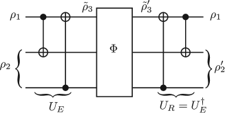
Figure 1: Encoding circuit $U_{E}$, error channel $\Phi$ and recovery circuit $U_{R}$ in the simplest case.

Let $\mathcal{S}_{1}$ and $\mathcal{S}_{2}$ be the state spaces of the data qubit and the ancillae, respectively. The set of the encoded states $\tilde{\mathcal{S}}_{3}=U_{E}(\mathcal{S}_{1}\otimes\mathcal{S}_{2})U_{E}^{\dagger}$ is a subset of the total state space $\mathcal{S}_{3}$ of the three-qubit system. How our QEC scheme works is summarized in Fig. 2.

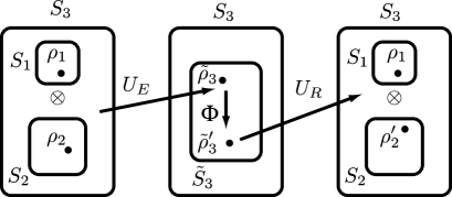
Figure 2: Encoding operator $U_{E}$ maps a tensor product state $\rho_{1}\otimes\rho_{2}\in{\mathcal{S}_{1}}\otimes{\mathcal{S}}_{2}$ to a codeword $\tilde{\rho}_{3}\in\tilde{{\mathcal{S}}}_{3}$. The error channel ${\Phi}$ maps $\tilde{\rho}_{3}$ to $\tilde{\rho}_{3}^{\prime}$ within the code space $\tilde{{\mathcal{S}}}_{3}$. As a result, the recovery operator $U_{R}$ maps $\tilde{\rho}_{3}^{\prime}$ to $\rho_{1}\otimes\rho_{2}^{\prime}$, restoring the data qubit.

The extreme case of the uniformly mixed state $\rho_{2}=\sigma_{0}^{\otimes 2}/4$ is worth analyzing separately. When the data qubit is in a pure state, this provides an interesting example of DQC-1 dqc1 . Moreover, our QEC scheme equally works for a data qubit in a mixed initial state. It is readily found that

$$U_{R}{\Phi}\left(U_{E}\left(\rho_{1}\otimes\frac{\sigma_{0}^{\otimes 2}}{4}\right)U_{E}^{\dagger}\right)U_{R}^{\dagger}=\rho_{1}\otimes\frac{\sigma_{0}^{\otimes 2}}{4}.$$ (6)

This shows that $\rho_{1}\otimes\sigma_{0}^{\otimes 2}/4$ is a fixed point of this operation for any $\rho_{1}\in\mathcal{S}_{1}$.

Let us compare our QEC scheme with the NS encoding scheme discussed in qecc3 . This NS encoding scheme employs three qubits to encode a logical qubit robust against any noise of the form $W^{\otimes 3}$, where $W$ is an arbitrary element of the 2-dimensional representation of SU(2). It was shown for this scheme that

$$U^{\prime}_{R}{\Phi^{\prime}}\left(U^{\prime}_{E}(\rho_{1}\otimes|0\rangle\langle 0|\otimes\rho_{a}){U^{\prime}_{E}}^{\dagger}\right){U^{\prime}_{R}}^{\dagger}$$

$$= \rho_{1}\otimes|0\rangle\langle 0|\otimes\sum_{i=0}^{3}p_{i}U_{i}\rho_{a}U_{i}^{\dagger},$$

where $U^{\prime}_{E}$ and $U^{\prime}_{R}$ are the encoding and the recovery operators, respectively. $\{U_{i}\}=\{\sigma_{0},e^{i\alpha\sigma_{x}},e^{i\beta\sigma_{y}},e^{i\gamma\sigma_{z}}\}$ is the set of error operators and $\Phi^{\prime}$ is defined by an expression analogous to Eq. (3). For this scheme, the initial ancilla state is required to be of the form $|0\rangle\langle 0|\otimes\rho_{a}$. In contrast, although the error operators avoidable with our scheme are restricted within a subset of those avoidable in qecc3 , our proposal has the remarkable advantage that any initial ancilla state $\rho_{2}$ can be employed for successful QEC.

We will discuss quantum discord (hereafter, abbreviated as QD) introduced in QD in order to analyze another aspect of our scheme. QD is a measure of non-classical correlations between two subsystems of a quantum system. Surprisingly enough, it was found that QD may be non-vanishing even in the absence of entanglement and that in fact, there are useful quantum algorithms that work with little or no entanglement called DQC-1 dqc1 ; Zeeya ; DQC1QD . In other words, separability alone does not imply the absence of a quantum nature of the state.

The left and the right QDs of our encoded state

$$\tilde{\rho}_{3} = \frac{1}{8}\left(\sigma_{0}\otimes\sigma_{0}\otimes\sigma_{0}+n_{x}\sigma_{x}\otimes\sigma_{x}\otimes\sigma_{0}\right.$$ (7)

$$+ \left.n_{y}\sigma_{y}\otimes\sigma_{x}\otimes\sigma_{z}+n_{z}\sigma_{z}\otimes\sigma_{0}\otimes\sigma_{z}\right),$$

are defined respectively as QD ; DVB

$$\mathcal{D}(2:1) = S(\tilde{\rho}_{1})-S(\tilde{\rho}_{3})+\tilde{S}(2|1),$$

$$\mathcal{D}(1:2) = S(\tilde{\rho}_{2})-S(\tilde{\rho}_{3})+\tilde{S}(1|2).$$

Note that they are not necessarily equal to each other QD . Here, $S(\rho)\equiv-{\rm Tr}(\rho\log_{2}\rho)$ is the von Neumann entropy of a density matrix $\rho$. The density matrices $\tilde{\rho}_{1}$ and $\tilde{\rho}_{2}$ are obtained by tracing over the ancillae and data-qubit states, respectively. We define a projective measurement by a complete set of two orthonormal vectors $\displaystyle\{|\pm\bm{m}\rangle\}$, which define $\displaystyle|\pm\bm{m}\rangle\langle\pm\bm{m}|=\frac{\sigma_{0}\pm\bm{m}\cdot\bm{\sigma}}{2}$ with $|\bm{m}|=1$. Let us define the conditional entropy by $\displaystyle S_{\{|\pm\bm{m}\rangle\}}(2|1)=\sum_{\pm}p_{\pm}S(\rho_{2|\pm})$, where $\rho_{2|\pm}=\langle\pm\bm{m}|\tilde{\rho}_{3}|\pm\bm{m}\rangle/p_{\pm}$ and $p_{\pm}={\rm Tr}\langle\pm\bm{m}|\tilde{\rho}_{3}|\pm\bm{m}\rangle$. Then, $\tilde{S}(2|1)$ is defined as $\displaystyle\min_{|\bm{m}|=1}S_{\{|\pm\bm{m}\rangle\}}(2|1)$. $\tilde{S}(1|2)$ is defined similarly.

The explicit form of the ancilla state after the measurement of the data qubit with a basis $\{|\pm\bm{m}\rangle\}$ is

$$\rho_{2|\pm} = \frac{1}{4}\left(\sigma_{0}\otimes\sigma_{0}\pm n_{x}m_{x}\sigma_{x}\otimes\sigma_{0}\right.$$

$$\pm n_{y}m_{y}\sigma_{x}\otimes\sigma_{z}\pm n_{z}m_{z}\sigma_{0}\otimes\sigma_{z}\left.\right).$$

The corresponding conditional entropy is

$$S_{\{|\pm\bm{m}\rangle\}}(2|1) = 2-\frac{1}{8}\sum_{j=1}^{8}(1+\bm{n}\cdot\bm{n}_{j})\log_{2}(1+\bm{n}\cdot\bm{n}_{j}),$$

where $\bm{n}_{j}=(\pm m_{x},\pm m_{y},\pm m_{z})$ are all eight combinations of three $\pm$.

Figure 3: Example of $\mathcal{D}_{\{|\pm\bm{m}\rangle\}}(2:1)$ when the initial state of the data qubit has the Bloch vector $\bm{n}=\hat{\bm{x}}$. $(r,\theta_{m},\phi_{m})=\left(\mathcal{D}_{\{|\pm\bm{m}\rangle\}}(2:1),\theta_{m},\phi_{m}\right)$ is plotted, where $\theta_{m}$ and $\phi_{m}$ specify $\bm{m}=(\sin\theta_{m}\cos\phi_{m},\sin\theta_{m}\sin\phi_{m},\cos\theta_{m})$. $\mathcal{D}_{\{|\pm\bm{m}\rangle\}}(2:1)=0$ for $\bm{m}=\pm\hat{\bm{x}}$. Therefore, $\mathcal{D}(2:1)$ vanishes for $\bm{n}=\hat{\bm{x}}$.

As an example, we show $\mathcal{D}_{\{|\pm\bm{m}\rangle\}}(2:1)=S(\tilde{\rho_{1}})-S(\tilde{\rho_{3}})+S_{\{|\pm\bm{m}\rangle\}}(2|1)$ for the initial state $\rho_{1}$ with the Bloch vector $\bm{n}=\hat{\bm{x}}$ as a function of $\bm{m}=(\sin\theta_{m}\cos\phi_{m},\sin\theta_{m}\sin\phi_{m},\cos\theta_{m})$ in Fig. 3. Here, $\hat{\bm{x}},\hat{\bm{y}}$ and $\hat{\bm{z}}$ are the unit vectors along the $x$-, $y$- and $z$-axes, respectively. Note that when $\bm{m}=\hat{\bm{x}}$, $\mathcal{D}_{\{|\pm\bm{m}\rangle\}}=0$. Therefore, $\mathcal{D}(2:1)=0$. The quantum discord $\mathcal{D}(2:1)$ as a function of $\bm{n}=(\sin\theta\cos\phi,\sin\theta\sin\phi,\cos\theta)$ is shown in Fig. 4.

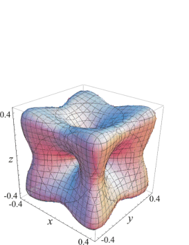
Figure 4: Quantum discord $\mathcal{D}(2:1)$ as a function of the initial state of the data qubit parameterized by the Bloch vector $\bm{n}=(\sin\theta\cos\phi,\sin\theta\sin\phi,\cos\theta)$. See Eq. (1). Coordinates $(r=\mathcal{D}(2:1),\theta,\phi)$ depict QD as a function of $\theta,\phi$. $\mathcal{D}(2:1)$ vanishes when $\bm{n}=(\pm 1,0,0),(0,\pm 1,0),(0,0,\pm 1)$. The function $\mathcal{D}(2:1)$ takes the maximum value $(3/4)\log_{2}3-1/2$ when $\bm{n}=(\pm 1,\pm 1,\pm 1)/\sqrt{3}$.

Although extensive optimization is necessary to evaluate QD in general, some initial states satisfying $\mathcal{D}(2:1)=0$ are easily obtained by carefully inspecting the structure of $\tilde{\rho}_{3}$. Let us consider the case $\bm{n}=\hat{\bm{x}}$, for example. In this case, $\tilde{\rho}_{3}$ is reduced to $\frac{1}{8}\left(\sigma_{0}\otimes\sigma_{0}\otimes\sigma_{0}+\sigma_{x}\otimes\sigma_{x}\otimes\sigma_{0}\right)$, which contains only $\sigma_{0}$ and $\sigma_{x}$ for the data qubit. Therefore, it is reasonable to employ $|\hat{\bm{x}}\rangle$ as a candidate for $|\bm{m}\rangle$ for obtaining $\tilde{S}(2|1)$. With this choice, $\tilde{\rho}_{3}$ is reduced to a block-diagonal form

$$\tilde{\rho}_{3}(\bm{n}=\hat{\bm{x}}) = \sum_{\pm}|\pm\hat{\bm{x}}\rangle\langle\pm\hat{\bm{x}}|\otimes\left(p_{\pm}\,\rho_{2|\pm}\right)$$

and $\mathcal{D}(2:1)=0$ is readily obtained QD ; DVB .

$\mathcal{D}(1:2)=0$ for an arbitrary initial state can be proved similarly. $\tilde{\rho}_{3}$ contains only $\sigma_{0}\otimes\sigma_{0}$, $\sigma_{x}\otimes\sigma_{0}$, $\sigma_{0}\otimes\sigma_{z}$, and $\sigma_{x}\otimes\sigma_{z}$ for the ancilla qubits. Therefore, we take

$$|\Pi_{\pm\pm}\rangle\langle\Pi_{\pm\pm}| = |\pm\hat{\bm{x}},\pm\hat{\bm{z}}\rangle\langle\pm\hat{\bm{x}},\pm\hat{\bm{z}}|=\frac{\sigma_{0}\pm\sigma_{x}}{2}\otimes\frac{\sigma_{0}\pm\sigma_{z}}{2}$$

as a complete set of four unit vectors that determine the projective measurement on the ancillae, although there are many other possibilities. $\tilde{\rho}_{3}$ is rewritten as

$$\tilde{\rho}_{3} = \sum_{\pm\pm}\left(p_{\pm\pm}\,\rho_{1|\pm\pm}\right)\otimes|\Pi_{\pm\pm}\rangle\langle\Pi_{\pm\pm}|.$$

When the data qubit and ancillae are rearranged, the density matrix is rewritten as a block-diagonal form and thus $\mathcal{D}(1:2)=0$ is immediately obtained.

According to the classification introduced in oppen ; horo , vanishing $\mathcal{D}(1:2)$ implies that our encoded state has a quantum-classical correlation. Furthermore, in case $\mathcal{D}(2:1)$ also vanishes, $\tilde{\rho}_{3}$ has a product eigenbasis as we have shown above, and the encoded state has a classical-classical correlation, or, in other words, is (properly) classically correlated.

When the ancillae are pure, we find $\mathcal{D}(2:1)=\mathcal{D}(1:2)$, which is nothing but the entanglement entropy. For example,

$$\mathcal{D}(2:1)=\mathcal{D}(1:2)$$

$$= 2-(1-n_{z})\log_{2}(1-n_{z})-(1+n_{z})\log_{2}(1+n_{z}),$$

when $\rho_{2}=|\bm{z}\rangle\langle\bm{z}|\otimes|\bm{z}\rangle\langle\bm{z}|$.

We demonstrate our QEC scheme with a NMR quantum computer. We employ a JEOL ECA-500 NMR spectrometer jeol , whose hydrogen Larmor frequency is approximately 500 MHz. We employ a linearly aligned three-spin molecule, ¹³C-labeled L-alanine (98% purity, Cambridge Isotope) solved in D₂O.

We simplify the quantum circuit shown in Fig. 1 by taking into account the fact that the phases of states are not independently observed in a NMR quantum computer. Both the encoding and the decoding require only 5 pulses including refocusing pulses, taking approximately 25 ms.

The density matrix of the thermal state is well approximated by

$$\rho = (\sigma_{0}/2)^{\otimes 3}$$

$$+ \frac{\epsilon}{8}\left(\sigma_{z}\otimes\sigma_{0}\otimes\sigma_{0}+\sigma_{0}\otimes\sigma_{z}\otimes\sigma_{0}+\sigma_{0}\otimes\sigma_{0}\otimes\sigma_{z}\right),$$

where $\epsilon\sim 10^{-6}$. Since $(\sigma_{0}/2)^{\otimes 3}$ is not visible in NMR, the density matrix of the thermal state is considered as a pseudo-pure state for DQC-1.

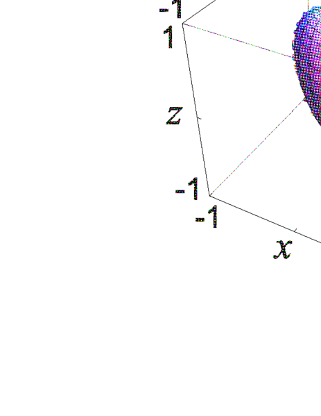
Error Operator	$X_{0}$	$X_{1}$	$X_{2}$
$F_{e}(\sigma_{0},{\mathcal{M}})$	$0.68$	$0.73$	$0.75$
${\rm Tr}({\mathcal{M}})$	$1.03$	$1.00$	$1.00$

Figure 5: Visualization of error correction performances. The surface of the Bloch sphere is mapped onto the surfaces in (a), (b) and (c) corresponding to three different error operators, $X_{0},X_{1},X_{2}$, respectively. See the text for details. Entanglement fidelities $F_{e}(\sigma_{0},\mathcal{M})$ and traces ${\rm Tr}({\mathcal{M}})$ are summarized in the table. ${\mathcal{M}}$ represents a map which is determined by the encoding, error, and recovery processes depicted in Fig. 1.

We perform three sets of experiments, in which we set

$$\begin{array}[]{ccc}(a)&\{p_{i}\}=(1,0,0,0)&:{\rm no~{}error}\\ (b)&\{p_{i}\}=(0,1,0,0)&:X_{1}{\rm~{}error}\\ (c)&\{p_{i}\}=(0,0,1,0)&:X_{2}{\rm~{}error},\end{array}$$

respectively, in Eq. (3). We do not need to examine the $X_{3}$ error separately since $X_{3}=iX_{2}~{}X_{1}$. Each set starts with 4 different initial states in order to apply quantum process tomography kondo . The results are summarized in Fig. 5. Although the surfaces are distorted, it is clear that our QEC scheme indeed eliminates the effects of the fully correlated noises. The table in Fig. 5 summarizes the entanglement fidelities.

It is noteworthy that one-qubit gate operations on the logical qubit take simple forms. Let $V$ be a one-qubit gate acting on the logical qubit. Then its action on the physical qubits is obtained by simplifying $U_{E}(V\otimes\sigma_{0}\otimes\sigma_{0})U_{R}$. For the simple gates $V=\sigma_{x},\sigma_{y}$ and $\sigma_{z}$, the corresponding operations on the physical qubits are $\sigma_{x}\otimes\sigma_{x}\otimes\sigma_{0},\sigma_{y}\otimes\sigma_{x}\otimes\sigma_{z},$ and $\sigma_{z}\otimes\sigma_{0}\otimes\sigma_{z},$ respectively. Note that these operators satisfy the ordinary $\mathfrak{su}(2)$ algebra. It is easy to obtain more general gate operations acting on the physical qubits by simply exponentiating these operators, e.g., $e^{-i\alpha\sigma_{x}\otimes\sigma_{x}\otimes\sigma_{0}}$ implements $V=e^{-i\alpha\sigma_{x}}$. Note that $e^{-i\beta\sigma_{y}\otimes\sigma_{x}\otimes\sigma_{z}}=e^{-i\pi(\sigma_{z}\otimes\sigma_{0}\otimes\sigma_{z})/4}e^{-i\beta\sigma_{x}\otimes\sigma_{x}\otimes\sigma_{0}}e^{i\pi(\sigma_{z}\otimes\sigma_{0}\otimes\sigma_{z})/4}$ in the case of $V=e^{-i\beta\sigma_{y}}$. From these operators, we can understand how the information of the data qubit is distributed in the encoded state. We note that direct operations on logical qubits in DFS/NS were discussed in gates_in_DFS .

In summary, we demonstrated a quantum error correction scheme avoiding fully correlated errors, in which the ancillae can be in a uniformly mixed state. Our results pave the way to new applications of DQC-1 to quantum computing. The analysis of quantum discord reveals that our encoding creates an interesting quantum correlation between the data qubit and the ancilla qubits; our encoded state has a quantum-classical correlation in general and has a classical-classical correlation when both left and right quantum discords vanish. We anticipate further progress both in the understanding of quantum correlations and the development of QEC schemes. Our QEC scheme admits simple one-qubit gate operations on the encoded qubits.

We are grateful to Hiroyuki Tomita for his valuable inputs and to Akira SaiToh for his critical reading. We are also grateful to the ‘Open Research Center’ Project for Private Universities, matching fund subsidy from the MEXT (Ministry of Education, Culture, Sports, Science and Technology) for financial support. Y. K. and M. N. would like to thank partial supports of Grants-in-Aid for Scientific Research from the JSPS (Grant No. 23540470). C. B. is supported by the MEXT Scholarship for foreign students.

References

(1)
F. Gaitan, Quantum Error Correction and Fault Tolerant Quantum Computing
(CRC Press, New York, 2008).
(2)
D. P. DiVincenzo,
Fortschritte der Physik 48, 771 (2000).
(3)
B. Criger, O. Moussa and R. Laflamme,
Phys. Rev. A 85, 044302 (2012).
(4)
C.-K. Li, M. Nakahara, Y.-T. Poon, N.-S. Sze and H. Tomita,
Phys. Rev. A 84, 044301 (2011).
(5)
H. Ollivier and W. H. Zurek, Phys. Rev. Lett. 88, 017901 (2001),
L. Henderson and V. Vedral, J. Phys. A 34, 6899 (2001).
(6)
E. Knill and R. Laflamme, Phys. Rev. Lett. 81,
5672 (1998).
(7)
Z. Merali, Nature, 474, 24 (2011).
(8)
E. Knill, R. Laflamme and L. Viola,
Phys. Rev. Lett., 84, 2525 (2000).
(9)
S. De Filippo, Phys. Rev. A 62, 052307 (2000).
(10)
C.-P. Yang and J. Gea-Banacloche, Phys. Rev. A 63,
022311 (2001).
(11)
J. Kempe, D. Bacon, D. A. Lidar and K. B. Whaley,
Phys. Rev. A 63, 042307 (2001).
(12)
P. Zanardi and M. Rasetti, Phys. Rev. Lett., 79, 3306
(1997).
(13)
P. Zanardi and M. Rasetti, Mod. Phys. Lett. B
11, 1085 (1997).
(14)
P. Zanardi, Phys. Rev. A 57, 3276 (1998).
(15)
D. A. Lidar, I. L. Chuang and K. B. Whaley,
Phys. Rev. Lett., 81, 2594 (1998).
(16)
G. Chiribella, M. Dall’Arno, G.M. D’Ariano, C. Macchiavello,
P. Perinotti, Phys. Rev. A 83, 052305 (2011).
(17)
C.-K. Li, M. Nakahara, Y.-T. Poon, N.-S. Sze, H. Tomita
Phys. Lett. A 375, 3255 (2011).
(18)
M. D. Reed, L. DiCarlo, S. E. Nigg, L. Sun, L. Frunzio,
S. M. Girvin and R. J. Schoelkopf,
Nature 482, 382 (2012).
(19)
A. Datta, A. Shaji, and C. M. Caves, Phy. Rev. Lett. 100,
050502 (2008).
(20)
B. Dakić, V. Vedral and C. Brukner,
Phys. Rev. Lett. 105, 190502 (2010).
(21)
J. Oppenheim, M. Horodecki, P. Horodecki and R. Horodecki, Phys. Rev. Lett.
89, 180402 (2002).
(22) M. Horodecki, P. Horodecki, R. Horodecki, J. Oppenheim,
A. Sen(De), U. Sen and B. Synak-Radtke, Phys. Rev. A 71, 062307 (2005).
(23)
http://www.jeol.com/.
(24)
See, for example, Y. Kondo,
J. Phys. Soc. Jpn. 76, 104004 (2007) and references therein.
(25) H. Barnum, M. A. Nielsen, and B. Schumacher, Phys. Rev. A
57, 4153 (1998).
(26) C. A. Bishop and M. S. Byrd,
J. Phys. A: Math. Theor. 42, 055301 (2009).