Controlling the Error Floor in LDPC Decoding

Abstract

The error floor of LDPC is revisited as an effect of dynamic message behavior in the so-called absorption sets of the code. It is shown that if the signal growth in the absorption sets is properly balanced by the growth of set-external messages, the error floor can be lowered to essentially arbitrarily low levels. Importance sampling techniques are discussed and used to verify the analysis, as well as to discuss the impact of iterations and message quantization on the code performance in the ultra-low BER (error floor) regime.

I Introduction

Low-density parity-check (LDPC) codes are a class of linear block codes [1] which have enjoyed intense theoretical and practical attention due to their excellent performance and decoding efficiency. Their parity-check matrices are given by sparse binary $(0,1)$ matrices which enable very efficient $O(n)$-complexity decoder implementations, where $n$ is the code length. The error rate of LDPC codes decreases rapidly as the signal-to-noise ratio (SNR) increases, and comes very close to maximum-likelihood (ML) decoding error performance, which is determined by the distance spectrum of the code.

However, when utilizing sub-optimal $O(n)$ iterative decoding algorithm, such as message passing (MP) or linear programming, a marked increase of error rates at high SNRs tends to appear with respect to optimal decoding. The error curve assumes the shape of an error floor with a very slow decrease with SNR. This error floor is caused by inherent structural weaknesses in the code’s interconnect network, which cause long latencies in the iterative decoder or outright lock-up in error patterns associated with these weaknesses. These decoding failures are very important for low-error-rate applications such as cable modems and optical transmission systems. They were initially studied in [2, 3, 4], and called trapping sets in [5]. Such trapping sets are dependent not only on the code but also on the channel where the code is used, as well as the specific decoding algorithm.

For example, trapping sets on the binary erasure channel are known as stopping sets [6], whereas the dominant trapping sets of LDPC codes on the Gaussian channel are the absorption sets [7]. Absorption sets are also the sets implicated in the failure mechanism of message-passing decoder for binary symmetric channels.

Due to the importance of error floors in low-BER applications, recent efforts have focused on understanding the dynamics of absorption sets [5, 8, 9, 10, 11, 12, 13, 14, 15], and several modifications of the decoding algorithm have been studied to lower the error floor, specifically targeting the absorption sets [16, 17, 12, 13]. As we discuss in this paper, the onset of the error floor on Gaussian channels is very strongly related to the behavior of the algorithm on binary symmetric channels, and that the dynamics of the absorption sets fully explain why and when the error floor becomes dominant in a given code.

In our earlier work [9, 11, 13] we developed a linear model to analyze dynamics of and probabilities for the error floor for specific codes. We identified and enumerated the minimal absorption sets, which dominate the decoding performance in the error floor region for the IEEE 802.3an and the Tanner $[155,64,20]$ codes, and derived closed-form formulas that approximate the probability that an absorption set falls in error.

In this paper, we first refine the formula for the error floor probability [9, 11, 13], and use it to show that the error floor critically depends on the limits, aka thresholds, which are utilized to represent the internal log-likelihood messages in the decoder. We show that the growth rate of the error patterns in the absorption set can be balanced by the growth of the LLRs external to the set, if a sufficient dynamic range for these messages is available. We quantify this effect and compare it to importance sampling guided simulations for verification. We verify the hypothesis that, quite unlike in the case of binary erasure or binary symmetric channels, the error floor phenomenon for LDPC codes on AWGN channels is essentially an “artifact” of inexact decoding, and not an inherent weakness of the code. We then quantify the effect of the number of iterations and show agreement of our refined equations with simulated error floor rates for both finite iterations and thresholds. Finally, we examine the impact of message quantization on the error floor and thus the required computational complexity to attain a given level of performance in the ultra-low BER regime of the code.

We wish to note that while sensitivity of the error floor to message thresholding has been observed heuristically by a number of authors, the view presented in this paper appears to have been developed independently by Butler and Siegel [14] as well as the authors [13, 9].

This paper is organized as follows: In Section II, LDPC codes, iterative decoding, and absorption sets are reviewed, and the two example LDPC codes used in our studies are introduced. In Section III, our linear algebraic approach to evaluate the error rate is described as a two-step procedure. The first step is to identify the dominant error patterns and the second is performing the analysis targeting these error patterns. Based on the insights provided by the analytical approach, Section IV studies different decoder settings for both the length-$155$ Tanner and the IEEE 802.3an LDPC codes. The computational complexity and importance sampling are discussed in Section V. Finally, the conclusion will be given in Section VI.

II Background

In this section, we first review the main features of LDPC codes and the most popular iterative decoding algorithms. Two LDPC codes will be introduced, as well. Then we apply the linear analysis technique of [9] to study their error floors in the following sections.

II-A LDPC Codes

An LDPC code is associated with a sparse parity-check matrix, denoted by $\mathbf{H}_{m\times n}$, where every column represents a code bit, and every row constitutes a parity-check equation. The code length is $n$, and the number of information bits $k\geq n-m$, since $\mathbf{H}$ is not necessarily full rank. If every column and every row of $\mathbf{H}$ has the same number of non-zero elements, then we have a “regular” LDPC code, otherwise the code is irregular. A regular LDPC code can also be represented by $(d_{v},d_{c})$, where $d_{v}$ and $d_{c}$ are the Hamming weights of each column and each row, respectively, together with an interleaver. Figure 1 shows the parity-check matrix of a $(3,5)$ regular LDPC code, where non-zero elements are plotted as solid dots and zeros are left blank.

Figure 1: The parity-check matrix of the Tanner $[155,64,20]$ regular $(3,5)$ LDPC code.

Following Tanner, an LDPC code can be represented by a bipartite graph, called a Tanner graph. Let check nodes denote the rows of the parity-check matrix, and variable nodes denote the columns of the matrix. Then every non-zero entry in $\mathbf{H}$ indicates a connection between these two disjoint sets.

II-A1 Tanner $[155,64,20]$ Regular $(3,5)$ LDPC Code

In [18] and [19], Tanner introduced a class of regular LDPC codes composed of blocks of circulant permutation matrices. The parity-check matrix $\mathbf{H}$ of these codes consists of a $d_{v}\times d_{c}$ array of such circulant permutation matrices $\mathbf{I}_{k}$, where each $\mathbf{I}_{k}$ denotes a $p\times p$ identity matrix with its rows shifted cyclically to the left by $k$ positions.

$$\mathbf{H}=\begin{bmatrix}[l]\mathbf{I}_{0,0}&\mathbf{I}_{0,1}&\cdots&\mathbf{I}_{0,d_{c}-1}\\ \mathbf{I}_{1,0}&\mathbf{I}_{1,1}&\cdots&\mathbf{I}_{1,d_{c}-1}\\ \vdots&\vdots&\ddots&\vdots\\ \mathbf{I}_{d_{v}-1,0}&\mathbf{I}_{d_{v}-1,1}&\cdots&\mathbf{I}_{d_{v}-1,d_{c}-1}\\ \end{bmatrix}_{d_{v}p\times d_{c}p}.$$ (1)

Immediately, we can tell that each row of (1) has exactly $d_{c}$, and each column $d_{v}$ non-zero elements, making the code a regular $(d_{v},d_{c})$ LDPC code. Its length is $d_{c}p$ and the number of check nodes is $d_{v}p$. Its “design” code rate is $1-d_{v}/d_{c}$, however the actual rate $R$ will be slightly higher in that within every row block, all $p$ rows add to an all-one vector and at least $d_{v}-1$ rows are linearly dependent.

The dimension of the base identity matrix $p$ was originally designed to be prime to eliminate $4$-cycles. In [19], $p$ was extended to non-primes, where the girth, the shortest cycle in the Tanner graph and denoted by $g$, can be as short as $4$. It can be shown that $g$ is upper bounded by $12$, no matter how large $n$ is [18, 20]. The minimum distance of a Tanner code is bounded by $d_{\min}\leq(d_{v}+1)!$ [21]. When $d_{v}$ is small, this upper bound can be met by carefully selecting the parameters [21, 19]. Tanner codes come with relatively large girth and/or minimum distance, and provide good error floor performance. However, low-weight absorption sets are not eliminated by this construction.

Tanner presented a $[155,64,20],(3,5)$ regular LDPC code in the “Recent Results” session of the IEEE International Symposium on Information Theory (ISIT) in 2000. Its block structure parity-check matrix is given by

$$\mathbf{H}=\begin{bmatrix}[l]\mathbf{I}_{1}&\mathbf{I}_{2}&\mathbf{I}_{4}&\mathbf{I}_{8}&\mathbf{I}_{16}\\ \mathbf{I}_{5}&\mathbf{I}_{10}&\mathbf{I}_{20}&\mathbf{I}_{9}&\mathbf{I}_{18}\\ \mathbf{I}_{25}&\mathbf{I}_{19}&\mathbf{I}_{7}&\mathbf{I}_{14}&\mathbf{I}_{28}\\ \end{bmatrix}_{93\times 155},$$ (2)

where each $\mathbf{I}_{x}$ is derived by shifting the rows of a $31\times 31$ identity matrix cyclically to the left by $x$ positions. Its binary structure is shown in Figure 1. This Tanner code has rate $R\approx 0.4129$ and is equipped with a large girth $g=8$ and $d_{\min}=20$ [18]. We will use this code as one of the examples to illustrate our error floor analysis.

II-A2 IEEE 802.3an $[2048,1723]$ Regular $(6,32)$ LDPC Code

The IEEE 802.3an RS-based low-density parity-check code belongs to a special class of binary linear block codes, constructed in [22, 23]. Its parity-check matrix is also comprised of blocks of permutation matrices:

$$\mathbf{H}=\begin{bmatrix}\sigma_{1,1}&\sigma_{1,2}&\cdots&\sigma_{1,32}\\ \sigma_{2,1}&\sigma_{2,2}&\cdots&\sigma_{2,32}\\ \vdots&\vdots&\ddots&\vdots\\ \sigma_{6,1}&\sigma_{6,2}&\cdots&\sigma_{6,32}\\ \end{bmatrix}_{384\times 2048},$$ (3)

where each $\sigma_{i,j}$ is a $64\times 64$ permutation matrix.

The design code rate is $1-d_{v}/d_{c}=0.8125$, whereas the actual code rate is slightly higher with $R=1723/2048\approx 0.8413$. The Tanner graph representing this code is $4$-cycle free and the minimal cycle length is $g=6$. We believe the minimum distance of this code is $14$ (it is either $12$ or $14$ [11]).

II-B Message-Passing Iterative Decoding Algorithms

Although ML decoding is optimal, it is too complex to implement. On the other hand, $O(n)$-iterative decoding performs extremely well. The idea of iterative decoding is that each check node combines all the information sent to it and returns a likelihood/suggestion back to the variable nodes connected to it. The variable nodes can either make a decision of the incoming messages, for example, a majority vote, or combine them up and send them back out to the check nodes for another iteration cycle. The process will stop when all check nodes are satisfied, i.e., a valid codeword is encountered, or the decoder reaches a maximum number of iterations allowed.

Decoding is monotonic in that the more iterations the decoder executes, the better the performance. This is strictly true for cycle-free codes. When the codes have cycles, the messages passing along the edges become dependent after a few iterations, which degrades the final decoding performance. Therefore, constructing a code with large girth is one way to guarantee good performance. In this paper a standard log-likelihood message-passing (MP) iterative decoding algorithm will be used as benchmark.

II-C LDPC Absorption Sets

The Gaussian channel differs from the binary symmetric channel and the binary erasure channel in that the dynamics of the error behavior of the LDPC decoder is more complicated. Richardson observed that the failure mechanism in the error floor of Gaussian channels was caused by what he called trapping sets [5]. But fully classifying trapping sets is a largely unsolved, and perhaps unsolvable, problem. Nonetheless, subsequent investigations noted that a special class of trapping sets, called absorption sets, dominates the error floor region [7, 10]. Furthermore, minimal absorption sets (see later) play a critical role in the error floor.

Definition 1.

An absorption set is a set of variable nodes such that the majority of the neighboring (connected) check nodes of each variable node in the set are connected to the set an even number of times.

Note 1.

The importance of absorption sets can easily be appreciated by realizing that Gallager’s original bit flipping decoding algorithm [1] will fail to correct an error pattern that falls onto an absorption set, and that such an error will therefore persist, even if the iteration count goes to infinity.

Let an ordered pair $(a,b)$ denote an absorption set where $a$ is size of the set and $b$ is the extrinsic message degree, i.e., the cardinality of the set (no repetition allowed) of the neighboring check nodes that are connected to the set an odd number of times (usually once). The belief that “smaller” absorption sets causes more severe effects on the error floor [5, 24] is supported by the analytical error floor equations derived in [9, 11]. This is analogous to the fact that lower weight codewords have more impact on the error rate than higher weight codewords.

III Error Floor Estimation

Our linear algebraic estimation process proceeds in two steps. First, the dominant absorption set topologies along with their multiplicities have to be identified for a given code. These are required to compute the dynamics of the sets in step two.

III-A Absorption Set Identification

There exist several papers on absorption set enumeration which make use of the topological features of the sets as well as algebraic properties used in the construction of the codes, [9, 11, 25, 10]. The search for absorption sets can be either algebraic or simulation-based, where the latter typically produces lower bounds on the multiplicities and set varieties. We have modified existing techniques and integrated them into our search method, in order to exhaustively enumerate the topologies and multiplicities in a systematic fashion for the more dominant sets up to a certain size, limited by computational complexity.

In the following, we list topological properties of the absorption sets of the Tanner $[155,64,20]$ and the IEEE802.3an $[2048,1723]$ LDPC codes, respectively.

III-A1 Tanner $[155,64,20],(3,5)$ LDPC Code

Following the enumerating methods in [9, 11], we list the first few absorption sets of the Tanner $[155,64,20],(3,5)$ LDPC code in TABLE I [13].

TABLE I: First few absorption sets of Tanner $[155,64,20],(3,5)$ code.

$a$	$b$	Existence	Multiplicity	Gain ($\mu_{\max}$)
$<4$		No
$4$	$4$	Yes	$465$	$1$
$5$	$1$	No
	$3$	Yes	$155$
	$5$		$3,720$
$6$	$2$	No
	$4$	Yes	$930$
	$6$		$22,630$	$1$
$7$	$1$	No
	$3$	Yes	$930$
	$5$		$16,275$
	$7$		$140,430$	$1$
$8$	$2$		$465$	$1.7870$
	$4$		$5,115$
	$6$		$196,540$
	$8$		$823,515$	$1$

Although the $(8,2)$ set is not the smallest absorption set in terms of $a$, it does have a small number of unsatisfied check nodes, which makes it dominant. Figure 2 shows the subgraph induced by the $(8,2)$ absorption set.

(a) Check nodes shown

(b) Check nodes hidden

Figure 2: The topology of the $(8,2)$ absorption set of the Tanner $[155,64,20]$ regular $(3,5)$ LDPC code (not all check node connections shown).

We observe from Figure 2(b) that the $(8,2)$ absorption set consists of cycles of length $8,10,12,14$ and $16$. In addition, it is also an extension set of lower weight absorption sets. As a matter of fact, all $(4,4)$, $(5,3)$, $(6,4)$ and $(7,3)$ sets are contained in $(8,2)$ sets. And $50\%$ of $(5,5)$, $4.1\%$ of $(6,6)$, $8.6\%$ of $(7,5)$ sets are contained in $(8,2)$ sets, respectively. We found that this $(8,2)$ set is the dominant absorption/trapping set of this Tanner code on the Gaussian channel under iterative MP decoding.

Actually, Figure 2(a) looks very much like a codeword in that, if all those eight variable nodes are erroneous and the rest of the variables in the code are correct, then all but two check nodes are unsatisfied.

$$\boldsymbol{\lambda} = \big{[}\underbrace{\lambda_{1},\lambda_{1},\lambda_{1},}_{\text{node \char 182}}\underbrace{\lambda_{2},\lambda_{2},\lambda_{2},}_{\text{node \char 183}}\underbrace{\lambda_{3},\lambda_{3},\lambda_{3},}_{\text{node \char 184}}\underbrace{\lambda_{4},\lambda_{4},}_{\text{node \char 185}}\underbrace{\lambda_{5},\lambda_{5},}_{\text{node \char 186}}\underbrace{\lambda_{6},\lambda_{6},\lambda_{6},}_{\text{node \char 187}}\underbrace{\lambda_{7},\lambda_{7},\lambda_{7},}_{\text{node \char 188}}\underbrace{\lambda_{8},\lambda_{8},\lambda_{8}}_{\text{node \char 189}}\big{]}^{\mathrm{T}}$$ (5)

$$\boldsymbol{\lambda}^{(\text{ex})}_{i} = \Big{[}\underbrace{0,0,0,}_{\text{node \char 182}}\underbrace{0,0,0,}_{\text{node \char 183}}\underbrace{0,0,0,}_{\text{node \char 184}}\underbrace{\lambda^{(\text{ex})}_{i4},\lambda^{(\text{ex})}_{i4},}_{\text{node \char 185}}\underbrace{\lambda^{(\text{ex})}_{i5},\lambda^{(\text{ex})}_{i5},}_{\text{node \char 186}}\underbrace{0,0,0,}_{\text{node \char 187}}\underbrace{0,0,0,}_{\text{node \char 188}}\underbrace{0,0,0}_{\text{node \char 189}}\Big{]}^{\mathrm{T}}$$ (6)

III-A2 IEEE 802.3an $[2048,1723]$ LDPC Code

Absorption sets up to size $a=10$ are listed in Table II [11].

TABLE II: The first few absorption sets of the IEEE 802.3an $[2048,1723]$, $(6,32)$ LDPC code.

$a$	$b$	Existence	Multiplicity	Gain ($\mu_{\max}$)
$<5$		No
$5$	$10$	No
$6$	$6$	No
	$8$
	$10$
	$12$
$7$	$0$	No
	$2$
	$4$
	$6$
	$8$
	$10$
	$12$	Yes	$65,472$	$3.29$
	$14$		$14,720$	$3$
$8$	$0$	No
	$2$
	$4$
	$6$
	$8$	Yes	$14,272$	$4$
	$10$	No
	$12$	Yes	$44,416$	$3.5$
	$14$		$88,896$	$3.25$
	$16$		$661,824$	$3$
$9$	$0$	No
	$2$
	$4$
	$6$
	$8$
	$10$
	$12$	Yes	?	$3.67$
	$14$			$3.44$
	$16$			$3.22$
	$18$			$3$
$10$	$0$	No
	$2$
	$4$
	$6$
	$8$	?
	$10$	Yes	$>192$	$4$
	$12$		?	$3.8$
	$14$			$3.6$
	$16$			$3.4$
	$18$			$3.2$
	$20$			$3$

The subgraph induced by the dominant $(8,8)$ absorption set is depicted in Figure 3. It can be seen that the topology is highly symmetric and also looks like a codeword. From Figure 3(a) one sees that only one-sixth of the neighboring check nodes will be unsatisfied when the set is in error. In addition, the graph shown in Figure 3(b) is also full of cycles of several lengths, similar to Figure 2(b).

(a) Check nodes shown

(b) Check nodes hidden

Figure 3: The topology of the dominant $(8,8)$ absorption set of the IEEE 802.3an code (not all check node connections shown).

The authors of [22] have shown that the minimum distance of this class of codes is lower bounded by $d_{\min}\geq d_{v}+1$ and has to be even. So we have $d_{\min}\geq 8$ for this IEEE 802.3an LDPC code. As a corollary of our absorption set enumeration, we tightened the lower bound to $d_{\min}>10$, because no $(a,0)$ absorption sets exist for $a\leq 10$ as seen in Table II [11]. In [25], it is shown that there are at least $1,407$ weight-$14$ codewords, found by an absorption set search algorithm. Therefore, the minimum distance is narrowed down to $d_{\min}=12$ or $14$.

III-B Linear Algebraic Estimation of the Error Rate

With the topologies and the multiplicities of the dominant absorption sets of both codes in hand, we proceed to approximate their contribution to the error rate.

III-B1 Tanner $[155,64,20],(3,5)$ LDPC Code

We apply the error formulation from [9, 11] to this Tanner code using the $(8,2)$ absorption set structure.

The variable nodes in Figure 2(a) are labeled from $1$ to $8$. We also label the solid edges from the variable nodes by $1,2,\dots,22$ one by one from left to right. Also denote the outgoing values from the variable nodes to the satisfied check nodes along these edges by $x_{i}$, for example, $x_{1},x_{2},x_{3}$ leave variable node ❶, $x_{4},x_{5},x_{6}$ variable node ❷, etc. Collect the $x_{i}$ in the length-$22$ column vector $\mathbf{x}$, which is the vector of outgoing variable edge values in the absorption set. Likewise, and analogously, let $\mathbf{y}$ be the incoming edge values to the variable nodes, such that $y_{j}$ corresponds to the reverse-direction message on edge $j$, $j=1,2,\dots,22$. Now, at iteration $i=0$,

$$\mathbf{x}_{0}=\boldsymbol{\lambda},$$ (4)

where the channel intrinsics vector $\boldsymbol{\lambda}$ is defined in (5). It undergoes the following operation at the check node:

$$\mathbf{y}_{0}=\mathbf{Cx}_{0}=\mathbf{C}\boldsymbol{\lambda},$$ (7)

where $\mathbf{C}$ is a permutation matrix that reflects the incoming messages back to the absorption set. By induction, we obtain at iteration $i=I$:

$$\mathbf{x}_{I}=\sum_{i=0}^{I}\left((\mathbf{VC})^{i}\boldsymbol{\lambda}+(\mathbf{VC})^{I-i}\boldsymbol{\lambda}_{i}^{(\text{ex})}\right),$$ (8)

where $\boldsymbol{\lambda}^{(\text{ex})}_{i}$ is the extrinsics vector and defined in (6), and the variable node addition matrix $\mathbf{V}$ is defined in (9). Note that $(\mathbf{VC})^{0}=\mathbf{I}$ and $\boldsymbol{\lambda}_{0}^{(\text{ex})}=\mathbf{0}$.

$$\mathbf{V} = \setcounter{MaxMatrixCols}{22}\begin{bmatrix}0&1&1&&&&&&&&&&&&&&&&&&&\\ 1&0&1&&&&&&&&&&&&&&&&&&&\\ 1&1&0&&&&&&&&&&&&&&&&&&&\\ &&&0&1&1&&&&&&&&&&&&&&&&\\ &&&1&0&1&&&&&&&&&&&&&&&&\\ &&&1&1&0&&&&&&&&&&&&&&&&\\ &&&&&&0&1&1&&&&&&&&&&&&&\\ &&&&&&1&0&1&&&&&&&&&&&&&\\ &&&&&&1&1&0&&&&&&&&&&&&&\\ &&&&&&&&&0&1&&&&&&&&&&&\\ &&&&&&&&&1&0&&&&&&&&&&&\\ &&&&&&&&&&&0&1&&&&&&&&&\\ &&&&&&&&&&&1&0&&&&&&&&&\\ &&&&&&&&&&&&&0&1&1&&&&&&\\ &&&&&&&&&&&&&1&0&1&&&&&&\\ &&&&&&&&&&&&&1&1&0&&&&&&\\ &&&&&&&&&&&&&&&&0&1&1&&&\\ &&&&&&&&&&&&&&&&1&0&1&&&\\ &&&&&&&&&&&&&&&&1&1&0&&&\\ &&&&&&&&&&&&&&&&&&&0&1&1\\ &&&&&&&&&&&&&&&&&&&1&0&1\\ &&&&&&&&&&&&&&&&&&&1&1&0\\ \end{bmatrix}_{22\times 22}.\hskip 14.22636pt$$ (9)

Both $\mathbf{C}$ and $\mathbf{V}$ are square matrices and share the dimension $ad_{v}-b$, which is the number of the solid edges in Figure 2(a).

Now we calculate the maximum eigenvalue $\mu_{\max}$ of $\mathbf{VC}$ and its corresponding unit-length eigenvector $\mathbf{v}_{\max}$ in (10), since they are dominating the magnitude of the power of $\mathbf{VC}$ in (8).

$$\mu_{\max}\approx 1.7870,\quad\mathbf{v}_{\max}=\begin{bmatrix}v_{1}\\ v_{2}\\ v_{3}\\ v_{4}\\ v_{5}\\ v_{6}\\ v_{7}\\ v_{8}\\ v_{9}\\ v_{10}\\ v_{11}\\ v_{12}\\ v_{13}\\ v_{14}\\ v_{15}\\ v_{16}\\ v_{17}\\ v_{18}\\ v_{19}\\ v_{20}\\ v_{21}\\ v_{22}\\ \end{bmatrix}\approx\begin{bmatrix}0.2369\\ 0.2369\\ 0.2273\\ 0.2031\\ 0.2031\\ 0.2651\\ 0.2254\\ 0.2254\\ 0.1660\\ 0.1261\\ 0.1483\\ 0.1483\\ 0.1261\\ 0.2031\\ 0.2651\\ 0.2031\\ 0.2369\\ 0.2369\\ 0.2273\\ 0.2201\\ 0.2201\\ 0.2544\\ \end{bmatrix}.$$ (10)

The large value of $\mu_{\max}$ also underscores the dominance of this $(8,2)$ absorption set over others listed in Table I.

Following [9, 11, 13], the $(8,2)$ absorption set falls in error if

$$\beta=\mathbf{x}_{I}^{\mathrm{T}}\cdot\mathbf{1}\leq 0.$$ (11)

$$P_{\rm AS} = Q\left(\frac{\displaystyle Am_{\lambda}\sum\limits_{i=0}^{I}\left(\frac{1}{\mu_{\max}^{i}}\prod_{l=0}^{i}\frac{1}{g_{l}}\right)+B\sum\limits_{i=1}^{I}\left(\frac{m_{\lambda^{(\text{ex})}}^{(i)}}{\mu_{\max}^{i}}\prod_{l=1}^{i}\frac{1}{g_{l}}\right)}{\displaystyle\sqrt{2Cm_{\lambda}\left(\sum\limits_{i=0}^{I}\left(\frac{1}{\mu_{\max}^{i}}\prod_{l=0}^{i}\frac{1}{g_{l}}\right)\right)^{2}+2D\sum\limits_{i=1}^{I}\left(\frac{m_{\lambda^{(\text{ex})}}^{(i)}}{\mu_{\max}^{2i}}\left(\prod_{l=1}^{i}\frac{1}{g_{l}}\right)^{2}\right)}}\right)$$ (25)

$$P_{\rm AS} = Q\left(\frac{\displaystyle 2m_{\lambda}\sum\limits_{i=0}^{I}\left(\frac{1}{\mu_{\max}^{i}}\prod_{l=0}^{i}\frac{1}{g_{l}}\right)+2\sum\limits_{i=1}^{I}\left(\frac{m_{\lambda^{(\text{ex})}}^{(i)}}{\mu_{\max}^{i}}\prod_{l=1}^{i}\frac{1}{g_{l}}\right)}{\displaystyle\sqrt{m_{\lambda}\left(\sum\limits_{i=0}^{I}\left(\frac{1}{\mu_{\max}^{i}}\prod_{l=0}^{i}\frac{1}{g_{l}}\right)\right)^{2}+\sum\limits_{i=1}^{I}\left(\frac{m_{\lambda^{(\text{ex})}}^{(i)}}{\mu_{\max}^{2i}}\left(\prod_{l=1}^{i}\frac{1}{g_{l}}\right)^{2}\right)}}\right)$$ (26)

For simplicity, we separate this expression into two parts, namely $\beta_{1}$ and $\beta_{2}$, as defined in (12).

$$\beta=\underbrace{\sum_{i=0}^{I}\left[(\mathbf{VC})^{i}\boldsymbol{\lambda}\right]^{\mathrm{T}}\cdot\mathbf{1}}_{\triangleq\beta_{1}}+\underbrace{\sum_{i=0}^{I}\left[(\mathbf{VC})^{I-i}\boldsymbol{\lambda}_{i}^{(\text{ex})}\right]^{\mathrm{T}}\cdot\mathbf{1}}_{\triangleq\beta_{2}}.$$ (12)

Let

$$A = \sum_{j=1}^{22}v_{j}$$ (13)

$$B = v_{10}+v_{11}+v_{12}+v_{13}$$ (14)

$$C = \left(v_{1}+v_{2}+v_{3}\right)^{2}+\left(v_{4}+v_{5}+v_{6}\right)^{2}+\left(v_{7}+v_{8}+v_{9}\right)^{2}$$ (15)

$$+\left(v_{10}+v_{11}\right)^{2}+\left(v_{12}+v_{13}\right)^{2}+\left(v_{14}+v_{15}+v_{16}\right)^{2}$$

$$+\left(v_{17}+v_{18}+v_{19}\right)^{2}+\left(v_{20}+v_{21}+v_{22}\right)^{2}$$

$$D = \left(v_{10}+v_{11}\right)^{2}+\left(v_{12}+v_{13}\right)^{2}$$ (16)

and apply the spectral theorem,

$$(\mathbf{VC})^{i}\boldsymbol{\lambda}\rightarrow\mu_{\max}^{i}\left(\boldsymbol{\lambda}^{\mathrm{T}}\mathbf{v}_{\max}\right)\mathbf{v}_{\max},$$ (17)

the means and the variances of $\beta_{1}$ and $\beta_{2}$, individually, simplify to (18)–(21).

$$m_{\beta_{1}} = A^{2}\sum_{i=0}^{I}\frac{1}{\mu_{\max}^{i}}m_{\lambda}$$ (18)

$$\sigma_{\beta_{1}}^{2} = 2A^{2}C\left(\sum_{i=0}^{I}\frac{1}{\mu_{\max}^{i}}\right)^{2}m_{\lambda}$$ (19)

$$m_{\beta_{2}} = AB\sum_{i=1}^{I}\frac{m_{\lambda^{(\text{ex})}}^{(i)}}{\mu_{\max}^{i}}$$ (20)

$$\sigma_{\beta_{2}}^{2} = 2A^{2}D\sum_{i=1}^{I}\frac{m_{\lambda^{(\text{ex})}}^{(i)}}{\mu_{\max}^{2i}}.$$ (21)

So, the probability of an absorption set falling in error is given by:

$$P_{\rm AS} = {\rm Pr}\left(\beta\leq 0\right)=Q\left(\frac{m_{\beta_{1}}+m_{\beta_{2}}}{\sqrt{\sigma^{2}_{\beta_{1}}+\sigma^{2}_{\beta_{2}}}}\right)$$ (22)

$$= \!Q\left(\!\frac{\displaystyle Am_{\lambda}\sum\limits_{i=0}^{I}\frac{1}{\mu_{\max}^{i}}+B\sum\limits_{i=1}^{I}\frac{m_{\lambda^{(\text{ex})}}^{(i)}}{\mu_{\max}^{i}}}{\displaystyle\sqrt{2Cm_{\lambda}\left(\sum\limits_{i=0}^{I}\frac{1}{\mu_{\max}^{i}}\right)^{2}\!\!\!+\!2D\sum\limits_{i=1}^{I}\frac{m_{\lambda^{(\text{ex})}}^{(i)}}{\mu_{\max}^{2i}}}}\!\right).\hskip 14.22636pt$$ (23)

As illustrated, the factors $A,B,C$ and $D$ are determined by the absorption set topology. Knowledge of $(a,b)$ and $d_{v}$ is encoded into them. For the Tanner code, $B$ or $D$ are much smaller than $A$ or $C$, compared to the case of the dominant absorption set of the IEEE 802.3an code [9, 11]. This implies that the critical extrinsic information has less impact on the error rate of the absorption set, which makes it more troublesome than the $(8,8)$ absorption set of the IEEE 802.3an code.

Exchanging extrinsic values at the black check nodes in Figure 2(a) is only a first order approximation of the actual messages returned, and the effect of the remaining $d_{c}-2$ inputs to these check nodes can be accounted for with an average, iteration-depended gain factor which was computed in [11] as

$$g_{l}=\mathbb{E}\left[\prod_{i=1}^{d_{c}-2}\tanh\left(\frac{m_{\mu^{(\mathrm{ex})}}^{(i)}}{2}\right)\right],$$ (24)

where $m_{\mu^{(\mathrm{ex})}}^{(i)}$ represents the mean of the signals $\mu^{(\mathrm{ex})}$ from the variable to the check nodes, and is computed using density evolution. With this refinement the probability in (23) is refined to (25). (Note that $g_{0}$ is set to $1$.) This check node gain quickly grows to $1$ after a few iterations, which implies that the external variable nodes have assumed their corrected values with correspondingly large LLR values.

III-B2 IEEE 802.3an $[2048,1723]$, $(6,32)$ LDPC Code

The IEEE 802.3an LDPC code’s dominant absorption set is shown in Figure 3 and has eigenvalue and eigenvector given by [11]:

$$\mu_{\max} = 4$$ (27)

$$\mathbf{v}_{\max} = \frac{1}{\sqrt{40}}\left[1,1,\dots,1\right]^{\mathrm{T}}_{40\times 1}.$$ (28)

The symmetry is also reflected in the following coefficients.

$$A = \sum_{j=1}^{40}v_{j}=B$$ (29)

$$C = \left(v_{1}+v_{2}+v_{3}+v_{4}+v_{5}\right)^{2}$$ (30)

$$+\left(v_{6}+v_{7}+v_{8}+v_{9}+v_{10}\right)^{2}$$

$$+\left(v_{11}+v_{12}+v_{13}+v_{14}+v_{15}\right)^{2}$$

$$+\left(v_{16}+v_{17}+v_{18}+v_{19}+v_{20}\right)^{2}$$

$$+\left(v_{21}+v_{22}+v_{23}+v_{24}+v_{25}\right)^{2}$$

$$+\left(v_{26}+v_{27}+v_{28}+v_{29}+v_{30}\right)^{2}$$

$$+\left(v_{31}+v_{32}+v_{33}+v_{34}+v_{35}\right)^{2}$$

$$+\left(v_{36}+v_{37}+v_{38}+v_{39}+v_{40}\right)^{2}=D.$$

Substituting (29) and (30) into (25), the probability of the $(8,8)$ absorption set falling in error is computed as (26), which is equivalent to setting $A=C=a=8$ and $B=D=b=8$.

III-C Error Probability Formula Refinement

Besides the relative simplicity of (23) and (25), one of the important insights we gain is that $\mu_{\max}$ and $\mathbf{v}_{\max}$ play a crucial role in the decoding failure mechanism. Absorption sets with large $\mu_{\max}$ have more impact on the code performance, since they accelerate the growth of erroneous LLRs within the set. The error formula can be strengthened, and in this section, we revisit its derivation to obtain a more accurate formula.

III-C1 $P_{\mathrm{AS}}$

We interpreted the probability of (11) happening as constituting the probability that an absorption set falls in error in [9, 11]. This condition can be strengthened because at the last iteration $I$, all elements of $\mathbf{x}_{I}$ are negative by virtue of (10). The failure probability is more accurately defined as

$$P_{\mathrm{AS}}=\Pr(\mathbf{x}_{I}\leq\mathbf{0}).$$ (31)

In addition, all elements of $\mathbf{x}_{I}$ are linear combinations of $\lambda_{1},\lambda_{2},\dots,\lambda_{a}$ and $\lambda^{(\mathrm{ex})}_{i,1},\lambda^{(\mathrm{ex})}_{i,2},\dots,\lambda^{(\mathrm{ex})}_{i,b}$, where $i=1,2,\dots,I$. Therefore, (31) is equivalent to saying that

$$P_{\mathrm{AS}}=\Pr\left(\max_{j=1}^{ad_{v}-b}(x_{I,j})\leq 0\right).$$ (32)

In other words, if the message with the maximum value is negative at the $I$-th iteration, then all the other variable nodes have negative LLRs as well.

Analogously, we rewrite (8) into two parts $\boldsymbol{\beta}_{1}$ and $\boldsymbol{\beta}_{2}$, but as vectors this time.

$$\boldsymbol{\beta}=\mathbf{x}_{I}=\underbrace{\sum_{i=0}^{I}(\mathbf{VC})^{i}\boldsymbol{\lambda}}_{\triangleq\boldsymbol{\beta}_{1}}+\underbrace{\sum_{i=0}^{I}(\mathbf{VC})^{I-i}\boldsymbol{\lambda}_{i}^{(\text{ex})}}_{\triangleq\boldsymbol{\beta}_{2}}.$$ (33)

Taking the mean of $\boldsymbol{\beta}_{1}$ and $\boldsymbol{\beta}_{2}$ we obtain

$$\mathbf{m}_{\boldsymbol{\beta}_{1}} = m_{\lambda}\sum_{i=0}^{I}(\mathbf{VC})^{i}\mathbf{1},$$ (34)

$$\mathbf{m}_{\boldsymbol{\beta}_{2}} = \sum_{i=0}^{I-1}m^{(I-i)}_{\lambda^{(\mathrm{ex})}}(\mathbf{VC})^{i}\mathbf{1}$$ (35)

for the $(8,8)$ absorption set of the IEEE 802.3an LDPC code, and

$$\mathbf{m}_{\boldsymbol{\beta}_{2}}=\sum_{i=0}^{I-1}m^{(I-i)}_{\lambda^{(\mathrm{ex})}}(\mathbf{VC})^{i}\big{[}0,\dots,0,\underbrace{1,1,}_{\text{node \char 185}}\underbrace{1,1,}_{\text{node \char 186}}0,\dots,0\big{]}^{\mathrm{T}}$$ (36)

as mean of $\boldsymbol{\beta}_{2}$ for the $(8,2)$ absorption set of the Tanner $[155,64,20]$ code.

It can be seen that the maximum entry of $\mathbf{v}_{\max}$ is dominating the elements of $\mathbf{m}_{\boldsymbol{\beta}_{1}}+\mathbf{m}_{\boldsymbol{\beta}_{2}}$.

In the case of the $(8,2)$ absorption set of the Tanner code, $v_{6}$ or $v_{15}$ are the maximum entries of $\mathbf{v}_{\max}$, as can be seen in (10). Thus (32) becomes

$$P_{\mathrm{AS}}=\Pr\left(\max_{j=1}^{22}(x_{I,j})\leq 0\right)=\Pr\left(x_{I,6}\leq 0\right).$$ (37)

And our refined error probability formula can be derived accordingly, using the same technique developed in Section III-B. It will retain the form of (25), but is more accurate.

For the IEEE 802.3an LDPC code, all $\mathbf{v}_{\max}$ entries have equal size, as shown in (28). Selecting any $v_{j}$ for (32) will result in (26) obtained using (11) and (22). Therefore, this modification will not affect the result for the IEEE 802.3an code in [9, 11], and

$$\Pr\left(\mathbf{x}_{I}^{\mathrm{T}}\cdot\mathbf{1}\leq 0\right)=\Pr\left(\max_{j}^{40}(x_{I,j})\leq 0\right).$$ (38)

III-C2 Spectral Approximation

In (25) and (26), we use the approximation

$$(\mathbf{VC})^{i}\boldsymbol{\lambda}\approx\mu_{\max}^{i}\left(\boldsymbol{\lambda}^{\mathrm{T}}\mathbf{v}_{\max}\right)\mathbf{v}_{\max},\quad i=1,2,\dots,I,$$ (39)

to estimate the power of $\mathbf{VC}$. This is not very accurate when $i$ is small. The results from the early iterations are of great importance. So we will drop this approximation and use the matrix formulation (34)–(36) when plotting error rate estimates.

III-C3 Numerical Results

The refined formula predicting the error floor of the Tanner $[155,64,20],(3,5)$ code is plotted in Figure 6 as solid curves. The circles are numerical results from importance sampling (IS) to support our algebraic analysis. Error rates for the IEEE 802.3an code are shown in Figure 5.

IV Error Floor Reduction

The error floor formula (25) can be used to look for contributing factors that come into play in the ultra-low BER regime.

The absorption set structure determines the magnitude of $\mu_{\max}$, which affects how fast the set LLRs grow. The coefficients $A$, $B$, $C$ and $D$ depend on the code structure, as shown in (13)–(16) and (29)–(30), and the topology of the absorption sets. The mean of the intrinsics $m_{\lambda}$ dependents soley on the channel LLR and has no impact on the error floor.

It is common understanding that simply increasing the maximum number of iterations will not solve the trapping set problem. This is because the absorption set will stabilize after a few iterations as soon as the clipping levels are reached by the growing LLR messages. This convergence to a bit-flipping operation is exemplified in Figure 4. From Note 1 now, the absorption set will remain in error even for $I\rightarrow\infty$.

Figure 4: The accumulated LLRs at an $(8,8)$ absorption set nodes of the IEEE 802.3an LDPC code versus iterations, assuming all-zero codeword transmitted.

The decisive variable in the error floor formula is $m_{\lambda^{(\mathrm{ex})}}$, the mean of the signals injected into the absorption set through its unsatisfied check nodes, shown in Figure 2(a) and Figure 3(a). It is evident from (25) that the argument of the $Q$-function can grow only if $m^{(i)}_{\lambda^{(\mathrm{ex})}}$ can outpace $\mu^{(i)}_{\max}$ as $i\rightarrow\infty$. Therefore, clipping of $m_{\lambda^{(\mathrm{ex})}}$ has a major impact on the error probability.

By density evolution the extrinsics represented by $m^{(i)}_{\lambda^{(\mathrm{ex})}}$ will grow to infinity, however, using

$$\lambda_{j\to i}=2\tanh^{-1}\left(\prod_{l\in V_{j}\backslash\{i\}}\tanh\left(\frac{\lambda_{l\to j}}{2}\right)\right)$$ (40)

in the decoding algorithm effectively clips $\lambda_{i}^{(\mathrm{ex})}$ due to numerical limitations of computing the inverse hyperbolic tangent of a number close to unity. This is observed and discussed in [14] as saturation. Therefore, instead of (40), we use the corrected min-sum algorithm [26], which computes the check-to-variable LLR as

$$\lambda_{j\to i}=\left(\min_{l\in V_{j}\backslash\{i\}}\left(\left|\lambda_{l\to j}\right|\right)+\mathrm{CT}\right)\prod_{l\in V_{j}\backslash\{i\}}\text{sign}\left(\lambda_{l\to j}\right),$$ (41)

where CT represents a correcting term dependent on the check node degree,

$$\mathrm{CT}=\left\{\begin{array}[]{ll}-\frac{\ln\left(d_{c}-1\right)}{4},&\text{if \ }\min_{l\in V_{j}\backslash\{i\}}\left|\lambda_{l\to j}\right|\geq\frac{3\ln\left(d_{c}-1\right)}{8};\\ 0,&\text{otherwise,}\end{array}\right.$$ (42)

to avoid the $\tanh(\cdot)$ calculation.

Figure 5 shows the error rates of the IEEE 802.3an LDPC code in its error floor region. The dashed curves plot (26) for $I=10$ and $m_{\lambda}$ and $m^{(i)}_{\lambda^{(\mathrm{ex})}}$ are bounded by $10$, which is the clipping threshold. The circles are the numerical results of importance sampling (IS) utilizing (41) with the same $I$ and LLR clipping threshold. When the threshold is increased to $100$, the error rate decreases as (26) predicts, also shown in Figure 5, and supported by IS simulation. The error rate further decreases with the even bigger LLR clipping value of 1,000.

Despite the high sensitivity of the formula to numerical issues, IS simulations and analytical results agree to within a few tenths of a dB over the entire range of $E_{b}/N_{0}$ values of interest.

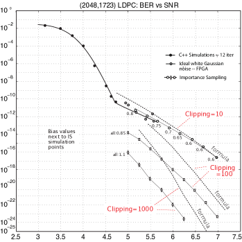
$E_{b}/N_{0}$

Figure 5: Bit error rates of the IEEE 802.3an LDPC code using both formula (26) and importance sampling (IS) with LLR clippings at 10, 100 and 1000, respectively. The iteration number is set to 10.

Regarding the short code, Figure 6 shows the error rates of the Tanner $[155,64,20]$ LDPC code. Once again, with higher LLR clipping value, (25) predicts that the error rate will decrease accordingly. This is supported by IS when the clipping threshold is raised from 10 to 100. However, the IS results of LLR clipped at 1,000 are not as low as suggested by (25), see the black stars in Figure 6. This is due to the short length of this code. Shortly after the decoding procedure begins, the LLRs will become so correlated that the extrinsics $\lambda_{i}^{(\mathrm{ex})}$ start to depart from the behavior predicted by density evolution. However, eventually, the absorption set is still corrected given more iterations are permitted [13]. The qualitative observations made above are therefore valid also for short codes, even though the quantitative prediction power of the error formulas breaks down.

$E_{b}/N_{0}$

Figure 6: Bit error rates of the Tanner $[155,64,20]$ LDPC code using both formula (25) and importance sampling (IS) with LLR clippings at 10, 100 and 1000, respectively. The maximum iteration number is set to 50.

V Iterations and Complexity

Larger LLR clipping thresholds imply more complexity in practice, since wider bit widths are needed to represent the messages. Figure 5 shows how much gain can be achieved by increasing the clipping values, in terms of lowering the error rate of the IEEE 802.3an LDPC code. We note that the theoretical results correlate well with the IS simulations.

Regarding the Tanner $[155,64,20]$ code, simply increasing the clipping threshold to over 100 alone has no additional benefit, as shown in Figure 6. The correlation among the LLRs of this small code compromise the growth of the extrinsic information entering the absorption sets.

Motivated by these observations, in this section we explore the impact of message quantization and number of iterations on a code’s error floor. Arguably, the product of bit-width and number of iterations is an accurate measure of the computational complexity of a decoder, since this number is directly related to the switching activity of a digital decoder (see [27]), and hence also the energy expended by the decoder.

In order to verify our theoretical results, we resort again to importance sampling (IS). IS is an ideal tool to explore variations of a decoder, such as finite precision operation, where the impact of design changes need to be explored for ultra-low error rates. Given the sensitivity of IS, we briefly discuss some major points here and relate our own experiences with IS applied to LDPC decoding.

Importance sampling is a method where one increases the number of significant events in low event-rate testing environments such as bit error rate testing or simulation. The basic principle of importance sampling is rooted in Monte-Carlo sampling. Specifically, here we wish to evaluate the probability that noise carries an original signal $x_{0}$ into the decision region of another signal, thus causing a decoding error. If $N_{s}$ noise samples are selected according to the channel’s noise distribution, an estimate of this error can be obtained as

$$\tilde{P}=\frac{1}{N_{s}}\sum_{i=1}^{N_{s}}w(y_{i}),$$ (43)

which is an unbiased estimate of the true error probability

$$P=\int_{\mathcal{D}}p(y|x_{0})\;dy,$$ (44)

where the weighting index is simply the error indicator

$$w(y)=\left\{\begin{array}[]{ccl}1,&&\text{if }y\in\mathcal{D};\\ 0,&&\text{otherwise}.\end{array}\right.$$ (47)

$\mathcal{D}$ is the signal space region where the decoder fails to produce the correct output $x_{0}$, and $p(y|x_{0})$ is the conditional probability density function of the received signal $y$ given the transmitted signal $x_{0}$, which is related to the noise distribution, for example, the Gaussian noise density in our case.

Unfortunately, for low values of $P$, one has to generate on the order of $10/P$ samples to obtain statistically relevant numbers of error events. For instance, the error floor of the IEEE 802.3an LDPC code appears below a bit error rate of $10^{-10}$, as shown in Figure 5, which requires $10^{11}$ to $10^{12}$ samples to be simulated and tested, and with lowering the error floor the number of test samples increases further.

One way of increasing the number of error events, or positive counts, is to distort the noise distribution to cause more errors. This is typically done by shifting the mean of the noise towards a convenient boundary of $\mathcal{D}$ (mean-shift importance sampling). The key questions are where to shift the transmitted signal and by how much.

A priori knowledge of the dominant error mechanisms is extremely important for proper use of IS, since otherwise a mean shift can actually mask an error by moving the signal further away from the dominant error event. Furthermore, the correct amount of the shift is also important. If the shift value is too small, not enough simulation speed up is achieved, if the shift value is too large, a phenomenon called over-biasing causes the IS error estimate to dramatically underestimate the true error contribution by the dominant event. This happens when the biased simulated samples occur too far away from the decision boundary, but inside the error region. These samples are weighed with a index that is too small. Not enough samples are generated close to the decision boundary from where the majority of the actual error contribution originates.

Since absorption sets are examined as the primary causes of the significant events in the error floor region, we add such a mean shift, or bias, towards the bits that make up the absorption set. Having identified and enumerated the dominant absorption sets of an LDPC code, we technically need to perform this shift for each absorption set separately, but symmetries can often be exploited in reducing this task. Gaussian distributed noise is added to the thus biased codeword $x_{0}$. As a result, the biased received $y$ will have an increased chance of causing an error by failing on the favored absorption set. Consequently the sample size $N_{s}$ can be significantly reduced, which translates into what is called “the gain” of importance sampling. Richardson [5] used a version of IS where this mean shift assumes a continuous distribution over which the simulations are averaged. This method appears to alleviate the over-biasing, but also obscures the phenomenon. In our approach we carefully choose the mean shift by assuring that small changes do not alter the computed error rate. Mean shift values used for some of our simulations are marked in the figures. We finally wish to note that, unlike sometimes implied in the literature, IS can only properly reproduce an error floor if the causes of the error floor are sufficiently well understood to apply proper biasing. Hence our two-step procedure in Section III.

Taking into account the bias value and the dominant absorption sets selected in the operation, the estimation formula (43) along with the weighting factor (47) must be adjusted accordingly, leading to a weight term $w(y)\ll 1$. The combined effect of measuring more significant events and ascribing them lower weight will produce the same error rate measure in (43) if the shifting is done correctly. Figs. 5 and 6 show the results of importance sampling for the IEEE 802.3an and the Tanner $[155,64,20]$ LDPC codes compared to our formulas for foating point calculations.

In a hardware implementation, however, finite precision arithmetic is used. The more digits used in the decoder, the more power and computational effort is required, but better performance will results. It is therefore vitally important for implementations to understand this cost-benefit tradeoff. For the IEEE 802.3an code, IS simulations with both floating and fixed point calculations at different LLR clipping values are shown in Figure 7. Not surprisingly, for smaller clipping values, smaller numbers of bits are required to adequately represent the messages. While 6 bits of quantization are required for a clipping threshold of 10, 10 bits are needed for a clipping threshold of 100, and 14 bits of quantization are required to exploit the full benefit of a clipping threshold of 1000.

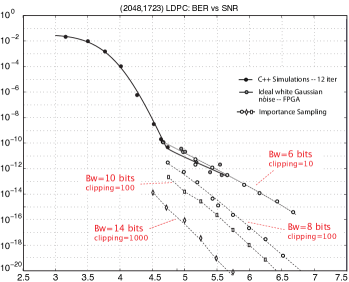
$E_{b}/N_{0}$

Figure 7: Error rates of the IEEE 802.3an LDPC code via importance sampling (IS) with finite precision, where the LLRs are clipped at 10, 100 and 1000, respectively. The maximum iteration number is preset at 10.

VI Conclusion

We revisited the error floor of LDPC codes and showed how the level of this floor can be controlled in a very large range by a proper choice of message representation inside the iterative message-passing decoder. In particular, the maximum allowed value of these messages, the clipping threshold, as well as the resolution of finite-precision arithmetic, have a key impact on the level of the floor. For short codes, additionally, very large iteration numbers may be required.

We verified our findings and error floor control mechanisms by extending our recent linearized analysis theory, and numerically verifying the results with importance sampling of the dominant absorption sets for two representative LDPC codes, namely the Tanner $[155,64,20]$ regular $(3,5)$ code and the larger IEEE 802.3an $[2048,1723]$ regular $(6,32)$ code. We conclude that the error floor can be lowered by many orders of magnitude, or made to virtually disappear, with proper setting of the message parameters, which allows the extrinsic signals to outpace the error growth inside the absorption sets.

References

• [1] R. G. Gallager, Low-Density Parity-Check Codes.   M.I.T. Press, Cambridge, MA, 1963.
• [2] N. Wiberg, “Codes and decoding on general graphs,” Ph.D. dissertation, Linköping University, Sweden, 1996.
• [3] B. J. Frey, R. Kötter, and A. Vardy, “Signal-space characterization of iterative decoding,” IEEE Trans. Inf. Theory, vol. 47, no. 2, pp. 766–781, Feb. 2001.
• [4] G. D. Forney, Jr., R. Kötter, F. R. Kschischang, and A. Reznik, “On the effective weights of pseudocodewords for codes defined on graphs with cycles,” in Codes, Systems, and Graphical Models, Springer, 2001, pp. 101–112.
• [5] T. J. Richardson, “Error floors of LDPC codes,” in 41st Annual Allerton Conference on Communications, Control and Computing, Oct. 2003, pp. 1426–1435.
• [6] C. Di, D. Proietti, I. E. Telatar, T. J. Richardson, and R. L. Urbanke, “Finite-length analysis of low-density parity-check codes on the binary erasure channel,” IEEE Trans. Inf. Theory, vol. 48, no. 6, pp. 1570–1579, June 2002.
• [7] Z. Zhang, L. Dolecek, B. Nikolic, V. Anantharam, and M. Wainwright, “Gen03-6: Investigation of error floors of structured low-density parity-check codes by hardware emulation,” in IEEE Global Telecommunications Conference, Dec. 2006, pp. 1–6.
• [8] J. Sun, O. Y. Takeshita, and M. P. Fitz, “Analysis of trapping sets for LDPC codes using a linear system model,” in 42nd Annual Allerton Conference on Communications, Control and Computing, Oct. 2004.
• [9] C. Schlegel and S. Zhang, “On the dynamics of the error floor behavior in regular LDPC codes,” in Information Theory Workshop, 2009. ITW 2009. IEEE, Oct. 2009, pp. 243–247.
• [10] L. Dolecek, Z. Zhang, V. Anantharam, M. Wainwright, and B. Nikolic, “Analysis of absorbing sets and fully absorbing sets for array-based LDPC codes,” IEEE Trans. Inf. Theory, vol. 56, no. 1, pp. 181–201, Jan. 2010.
• [11] C. Schlegel and S. Zhang, “On the dynamics of the error floor behavior in (regular) LDPC codes,” IEEE Trans. Inf. Theory, vol. 56, no. 7, pp. 3248–3264, July 2010.
• [12] J. Kang, Q. Huang, S. Lin, and K. Abdel-Ghaffar, “An iterative decoding algorithm with backtracking to lower the error-floors of LDPC codes,” IEEE Trans. Inf. Theory, vol. 59, no. 1, pp. 64–73, Jan. 2011.
• [13] S. Zhang and C. Schlegel, “Causes and dynamics of LDPC error floors on AWGN channels,” in Communication, Control, and Computing (Allerton), 2011 49th Annual Allerton Conference on, UIUC, Allerton Retreat Center, Monticello, IL, USA, Sept. 2011, pp. 1025 –1032.
• [14] B. K. Butler and P. H. Siegel, “Error floor approximation for LDPC codes in the AWGN channel,” in Communication, Control, and Computing (Allerton), 2011 49th Annual Allerton Conference on, UIUC, Allerton Retreat Center, Monticello, IL, USA, Sept. 2011, pp. 204 –211.
• [15] P. O. Vontobel, A list of references on pseudocodewords, trapping sets, stopping sets, absorption sets. [Online]. Available: http://www.pseudocodewords.info
• [16] M. Ivković, S. K. Chilappagari, and B. Vasić, “Eliminating trapping sets in low-density parity-check codes by using tanner graph covers,” IEEE Trans. Inf. Theory, vol. 54, no. 8, pp. 3763–3768, Aug. 2008.
• [17] Z. Zhang, L. Dolecek, B. Nikolic, V. Anantharam, and M. Wainwright, “Lowering LDPC error floors by postprocessing,” Global Telecommunications Conference, 2008. GLOBECOM ’08. IEEE, pp. 1–6, Dec. 2008.
• [18] R. M. Tanner, D. Sridhara, and T. E. Fuja, “A class of group-structured LDPC codes,” in Proc. Int. Symp Communications Theory and Applications, Ambleside, U.K., July 2001.
• [19] R. M. Tanner, D. Sridhara, A. Sridharanand, T. E. Fuja, and D. J. Costello, “LDPC block and convolutional codes based on circulant matrices,” IEEE Trans. Inf. Theory, vol. 50, no. 12, pp. 2966–2984, Dec. 2004.
• [20] M. P. C. Fossorier, “Quasicyclic low-density parity-check codes from circulant permutation matrices,” IEEE Trans. Inf. Theory, vol. 50, no. 8, pp. 1788–1793, Aug. 2004.
• [21] D. J. C. MacKay and M. C. Davey, “Evaluation of Gallager codes for short block length and high rate applications,” in Codes, Systems and Graphical Models, ser. IMA Volumes in Mathematics and its Applications, B. Marcus and J. Rosenthal, Eds.   New York: Springer, 2000, vol. 123, pp. 113–130.
• [22] I. Djurdjevic, J. Xu, K. Abdel-Ghaffar, and S. Lin, “A class of low-density parity-check codes constructed based on Reed-Solomon codes with two information symbols,” IEEE Commun. Lett., vol. 7, no. 7, pp. 317–319, July 2003.
• [23] L. Zeng, L. Lan, Y. Y. Tai, S. Lin, and K. Abdel-Ghaffar, “Construction of LDPC codes for AWGN and binary erasure channels based on finite fields,” in Information Theory Workshop, 2005 IEEE, August 29 – September 1, 2005, pp. 273–276.
• [24] S. Ländner and O. Milenkovic, “Algorithmic and combinatorial analysis of trapping sets in structured LDPC codes,” in Wireless Networks, Communications and Mobile Computing, 2005 International Conference on, vol. 1, 2005, pp. 630–635.
• [25] S. Abu-Surra, D. DeClercq, D. Divsalar, and W. E. Ryan, “Trapping set enumerators for specific LDPC codes,” in Information Theory and Applications Workshop (ITA), UCSD, San Diego, CA, USA, Feb. 2010, pp. 1–5.
• [26] S. L. Howard, C. Schlegel, and V. C. Gaudet, “Degree-matched check node decoding for regular and irregular LDPCs,” Circuits and Systems II: Express Briefs, IEEE Transactions on, vol. 53, no. 10, pp. 1054 –1058, Oct. 2006.
• [27] C. Schlegel, “From mathematics to physics: The task of building efficient and effective iterative error control decoders,” in the 7th International Symposium on Turbo Codes & Iterative Information Processing, Gothenburg, Sweden, August 27–31, 2012, invited plenary talk.