Computation of Effective Free Surfaces in Two Phase Flows

Abstract

In this investigation we revisit the concept of “effective free surfaces” arising in the solution of the time–averaged fluid dynamics equations in the presence of free boundaries. This work is motivated by applications of the optimization and optimal control theory to problems involving free surfaces, where the time–dependent formulations lead to many technical difficulties which are however alleviated when steady governing equations are used instead. By introducing a number of precisely stated assumptions, we develop and validate an approach in which the interface between the different phases, understood in the time–averaged sense, is sharp. In the proposed formulation the terms representing the fluctuations of the free boundaries and of the hydrodynamic quantities appear as boundary conditions on the effective surface and require suitable closure models. As a simple model problem we consider impingement of free–falling droplets onto a fluid in a pool with a free surface, and a simple algebraic closure model is proposed for this system. The resulting averaged equations are of the free–boundary type and an efficient computational approach based on shape optimization formulation is developed for their solution. The computed effective surfaces exhibit consistent dependence on the problem parameters and compare favorably with the results obtained when the data from the actual time–dependent problem is used in lieu of the closure model.

I Introduction

The goal of this work is to investigate the concept of “effective free surfaces” which are defined here as stationary interfaces corresponding to the time–averaged balance of mass, momentum and, if applicable, energy in a time–dependent flow with free surfaces. In other words, given an unsteady two–phase flow with fluctuating boundaries, the effective free surface represents the boundary between the two phases in the corresponding mean flow which satisfies the time–averaged form of the original system of governing equations subject to a number of modeling assumptions. The motivation for this work comes from the field of flow control g03 where many emerging applications involve control and optimization of free–surface phenomena. The particular applications underlying this research concern optimization of complex thermo–fluid phenomena occurring in liquid metals during welding, see Volkov et al.vplg09a . While the mathematical foundations for the optimal control of time–dependent free–boundary problems are relatively well understood mz06 , such approaches tend to result in computational problems of significant complexity even for simple models pl08 . The main difficulty arising when methods of the optimal control, or more broadly, the calculus of variations are applied to such problems is that some of the optimality conditions have the form of partial differential equations (PDEs) defined on interfaces which evolve with time. Needless to say, such problems tend to be quite hard to solve for non–trivial applications. On the other hand, this framework becomes much more tractable when time–independent free–boundary problems are considered instead hm03 . Moreover, on a more practical level, fluid flows with free surfaces may generate “subgrid–scale” features which are particularly difficult to compute, and it is therefore desirable to account for their effect in the average balance of mass and momentum in a systematic manner. In this paper we propose and test a simple mathematical model, in the form of a system of coupled PDEs of the free–boundary type, representing the time–averaged conservation of mass and momentum in a given time–dependent problem with free surfaces. While such averaging approaches are well–established in the study of turbulent flows in domains with fixed boundaries, giving rise to the well–known Reynolds–Averaged Navier–Stokes (RANS) equations, see, e.g., Popepope , the additional complication in the present problem is that one also needs to take into account the effect of the fluctuations of the location of the free surfaces on the average mass and momentum balance. Our approach to this problem relies on a number of simplifying assumptions which are all clearly identified. In the spirit of the “closure problem” arising in turbulence modeling, see Ref. pope, , in order to close the resulting system of equations one needs to express average products of fluctuating quantities in terms of average quantities. However, in contrast to the classical closure problem where the Reynolds stresses are modeled with terms defined in the bulk of the fluid, in the present problem, subject to certain assumptions, such closure terms will appear in the boundary conditions defined on the effective free boundary. We will also discuss some very simple strategies for constructing such closures. The question of ensemble–averaged, or time–averaged, description of flows with interfaces has received some attention in the literature and we mention here the work of Dopazo d77 , Hong & Walker hw00 and Brocchini & Peregrine bp01a ; bp01b which also contains references to a number of earlier attempts. These problems were recently revisited in the context of the derivation and validation of suitable models for multiphase Reynolds–averaged Navier–Stokes (RANS) equationsb02 and Large Eddy Simulation (LES) lltlvlcs07 ; tlls08 ; vlltls08 . We also mention the recent investigation by Wacławczyk & Oberlackwo11 where a number of closure strategies were proposed for this type of flows. Finally, we add that the related question of homogenization of free–boundary problems is an emerging topic in the mathematical analysis of PDEs, see, e.g., Schweizer s00 . A detailed description of various computational methods applied to multiphase flows can be found in the monograph by Prosperetti & Tryggvason prosperetti . As compared to these earlier studies, novel aspects of the present investigation are that, first, we want to compute steady–state solutions, which is motivated by the optimization applications mentioned above, and secondly, we want our averaged flows to feature sharp effective surfaces, so that the free–boundary property of the original problem is preserved in its averaged version. In contrast, we note that the formulations developed in Refs. bp01b, and wo11, lead to interfaces, referred to as “surface layers”, characterized by finite thickness. We also wish to highlight that although Brocchini & Peregrine bp01b derived averaged equations taking into account the fluctuations of the free boundaries and also proposed a simple closure model, to the best of our knowledge, there have been no attempts to actually compute such solutions for nontrivial problems which is one of the contributions of the present work.

The resulting system of PDEs represents the averaged balance of mass and momentum which has the form of a steady–state free–boundary problem. Since such problems tend to be difficult to solve numerically, we also propose a solution approach based on shape optimization which is well adapted to the numerical solution of this class of problems. In order to test our approach we choose a very simple model problem which, while allowing us to focus on certain methodological aspects, still captures some essential features of the motivating application, namely, the transfer of mass and momentum to the weld pool via droplets, see Figure 1. This model describes the two–dimensional (2D), time–periodic impingement of droplets on the free surface of the fluid in a container. In view of the comments made above, we see that formulation of an optimal control problem for the original time–dependent system would require us to satisfy certain optimality conditions on the boundary of each individual moving droplet in addition to conditions on the free surface of the liquid in the pool. On the other hand, the concept of the effective free surface allows us to replace this optimization problem with a simpler one, which is also computationally more tractable, where the optimality conditions have to be imposed on the stationary effective surfaces. Thus, as one application, the proposed approach will allow us to extend the optimization formulation developed in Volkov et al.vplg09a to include the effect of the mass transfer into the weld pool via droplet impingement.

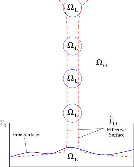
Figure 1: Schematic of our model problem representing droplets impinging on a free surface, a phenomenon typically encountered in various welding processes such as Gas–Metal Arc Welding (GMAW). The solid lines represent the actual time–dependent interface between the liquid and gas phases, whereas the dashed line is the steady effective surface $\tilde{\Gamma}_{LG}$ we seek to determine.

We remark that droplet impingement onto a thin liquid film is a phenomenon with manifold manifestations in technology, including chocolate processing, spray painting, corrosion of turbine blades, fuel injection in internal combustion engines, and aircraft icing. It also occurs in many natural phenomena such as the erosion of soil and the dispersal of spores and micro-organisms. A considerable amount of literature is available as concerns the numerical modeling of droplet impingement onto a solid surface. Harlow & Shannon harlow were the first to simulate this phenomenon and several other authors have applied the Volume–of–Fluid (VoF) based approaches such as RIPPLE ripple and SOLA–VOF hn81 to understand droplet impingement phenomena. Trujillo et al. trujillo also performed a numerical investigation and experimental characterization of the heat transfer from a periodic impingement of droplets.

The structure of this paper is as follows: in the next Section we present the formulation of the problem in general terms, in the following Section we introduce our model problem and in Section IV we discuss a very simple closure strategy which may be suitable for this problem, in Section V we introduce a shape–optimization approach to the numerical solution of the resulting averaged equations, whereas in Section VI we present some computational results together with a discussion; final conclusions are deferred to Section VII and some technical results concerning solution of the shape optimization problem in Section V are collected in Appendix A.

II Problem Formulation

In order to simplify the presentation of our approach, we will consider a two–dimensional problem formulated in a general domain $\Omega\subset\mathbb{R}^{2}$, shown schematically in Figure 2, where $\Omega_{L}$ and $\Omega_{G}$ represent the subdomains occupied, respectively, by the immiscible liquid and gas phases, whereas $\Gamma_{LG}$ represents the liquid–gas interface (e.g, droplet boundary or the free surface of the weld pool).

Figure 2: Schematic of the domains and domain boundaries used in the definition of the model problem in Section II.1. The domain $\Omega_{L}(t)$ occupied by the liquid phase is marked in gray, whereas the thin and thick solid lines represent, respectively, its boundary $\Gamma_{LG}(t)$ and the corresponding effective surface $\tilde{\Gamma}_{LG}$. The subregion $\Omega^{\prime}$ (see Section II.3) is delimited by the thick dashed lines.

II.1 Assumed Governing Equations

For a general description of the equations and boundary conditions governing multiphase flows we refer the reader to monograph by Prosperetti & Tryggvasonprosperetti . We assume that our model problem involves the following dependent variables

1. velocity $\textbf{v}=[u,v]^{T}\,:\,\Omega\times(0,T]\quad\to\mathbb{R}^{2}$,

2. pressure $p\,:\,\Omega\times(0,T]\quad\to\mathbb{R}$ and

3. position of the free surface $\forall_{t\in(0,T]},\ \Gamma_{LG}(t)\triangleq\overline{\Omega}_{L}(t)\cap\overline{\Omega}_{G}(t)$,

where $T$ denotes the length of the time window of interest and “$\triangleq$” means “equal to by definition”. It is also assumed that there is no mass transfer across the interface $\Gamma_{LG}$. We have the following equations governing the fluid flow in the two phases, for the moment in the time–dependent form

$$\rho_{L}{\partial{\mathbf{v}}\over\partial t}+\rho_{L}(\mathbf{v}\cdot\boldsymbol{\nabla})\mathbf{v}-\boldsymbol{\nabla}\cdot\boldsymbol{\sigma}-\rho_{L}{\mathbf{g}} =0\quad\text{in}\ \Omega_{L},$$ (1a)

$$\boldsymbol{\nabla}\cdot\mathbf{v} =0\quad\text{in}\ \Omega_{L},$$ (1b)

$$\rho_{G}{\partial{\mathbf{v}}\over\partial t}+\rho_{G}(\mathbf{v}\cdot\boldsymbol{\nabla})\mathbf{v}-\boldsymbol{\nabla}\cdot\boldsymbol{\sigma}-\rho_{G}{\mathbf{g}} =0\quad\text{in}\ \Omega_{G},$$ (2a)

$$\boldsymbol{\nabla}\cdot\mathbf{v} =0\quad\text{in}\ \Omega_{G},$$ (2b)

where $\rho_{L}$ and $\rho_{G}$ are the densities in the liquid and gas phase and $\boldsymbol{\sigma}\triangleq-p\mathbf{I}+\boldsymbol{\sigma}^{\mu}$ is the stress tensor in which $\boldsymbol{\sigma}^{\mu}\triangleq\mu\big{[}\boldsymbol{\nabla}\mathbf{v}+(\boldsymbol{\nabla}\mathbf{v})^{T}\big{]}$, $\mathbf{I}$ denotes the identity matrix and the viscosity coefficient $\mu=\mu_{L}$ or $\mu=\mu_{G}$ in the liquid and gas phase, respectively. The symbol ${\mathbf{g}}$ denotes the gravitational acceleration. Equations (1b) and (2b) represent conservation of mass, whereas equations (1a) and (2a) represent conservation of momentum in both the liquid and gas phase. Systems (1) and (2) are subject to the following boundary conditions on the liquid–gas interface $\Gamma_{LG}$

$$\mathbf{v}\big{|}_{L} =\mathbf{v}\big{|}_{G}\quad \textrm{on}\quad\Gamma_{LG},$$ (3a)

$$\Big{[}\boldsymbol{\sigma}\Big{]}_{L}^{G}.\mathbf{n} =\gamma\kappa\,\mathbf{n}\quad \text{on}\quad\Gamma_{LG},$$ (3b)

where ${\mathbf{n}}$ and ${\mathbf{t}}$ are the unit normal and tangential vectors on the interface $\Gamma_{LG}$, $\kappa$ is the interface curvature, $\gamma$ the surface tension (a material property assumed constant), whereas the subscripts $L$ and $G$ (with or without the vertical bar) denote quantities defined in the corresponding phases (Figure 2). We note that the vector–valued condition (3b) implies the balance of both the normal and tangential stresses. For simplicity, on the far boundary $\Gamma_{0}$, cf. Figure 2, we adopt the no–slip boundary condition

$${\mathbf{v}}\big{|}_{G}={\mathbf{0}}\qquad\textrm{on}\ \Gamma_{0}.$$ (4)

As regards the mathematical description of free–boundary problems, there are two main paradigms, namely, (i) “interface tracking” approaches, see Neittaanmaki et al. nst06 and (ii) “interface capturing” approaches, see Sethians96 . While description (1)–(3), featuring the location of the interface $\Gamma_{LG}$ as the dependent variable, belongs to the first category, for the purpose of developing our formulation an interface capturing approach will be more suitable and we employ a technique known as “Volume of Fluid” (VoF). However, our computations of the effective surfaces will be ultimately carried out with an “interface tracking” approach, see Section V. A detailed description of the VoF methodology can be found in the paper by Hirt & Nicholshn81 , see also monograph by Prosperetti & Tryggvason prosperetti . This method employs the “volume fraction” as an indicator function to mark different fluids

$$\forall_{t\in[0,T]}\qquad F({\mathbf{x}},t)=\left\{\begin{array}[]{ll}1&{\mathbf{x}}\in\Omega_{L}\\ 0&{\mathbf{x}}\in\Omega_{G}\end{array}\right..$$ (5)

While in the continuous setting the interface $\Gamma_{LG}$ is sharp and the VoF function $F$ may take the values of 0 and 1 only, in a numerical approximation there may exist a transition region where $0<F<1$ and the fluid can be treated as a mixture of the two fluids on each side of the interface. The values of the indicator function are associated with each fluid and hence are propagated as Lagrangian invariants. Therefore, the indicator function obeys a transport equation of the form

$$\frac{\partial F}{\partial t}+(\mathbf{v}\cdot\boldsymbol{\nabla})F=0\qquad\textrm{in}\ \Omega.$$ (6)

Based on the indicator function, local material properties such as the density $\rho$ of the fluid can be expressed as

$$\rho(F({\mathbf{x}}))=F({\mathbf{x}})\rho_{L}+[1-F({\mathbf{x}})]\rho_{G}.$$ (7)

Relationship (7) allow us to rewrite formulation (1)–(3) in an equivalent form as one system of conservation equations defined in the entire flow domain $\Omega$ where the fluid properties are, in general, discontinuous across the interface between the two fluids. In this single–field representation the two fluids are identified by indicator function (5), whereas the material properties are expressed as piecewise constant functions and can be written in terms of their values on either side of interface $\Gamma_{LG}$, cf. (7).

$${\partial\rho(F)\over\partial t}+\boldsymbol{\nabla}\cdot\left[\rho(F)\,\mathbf{v}\right] =0 \text{in}\ \Omega,$$ (8a)

$$\frac{\partial\rho(F)\,\mathbf{v}}{\partial t}+\boldsymbol{\nabla}\cdot\left[\rho(F)\,\mathbf{v}\mathbf{v}\right] =\boldsymbol{\nabla}\cdot\boldsymbol{\sigma}+\int_{\Gamma_{LG}}\gamma\kappa\,{\mathbf{n}}\delta({\mathbf{x}}-{\mathbf{x}}^{\prime})\,ds({\mathbf{x}}^{\prime})\quad \text{in}\ \Omega,$$ (8b)

$$\frac{\partial F}{\partial t}+(\mathbf{v}\cdot\boldsymbol{\nabla})F =0 \textrm{in}\ \Omega,$$ (8c)

where $\mathbf{v}\mathbf{v}$ denotes the dyadic product, i.e., the tensor defined as $\left[\mathbf{v}\mathbf{v}\right]_{ij}=\left[\mathbf{v}\right]_{i}\left[\mathbf{v}\right]_{j}$, $i,j=1,2$. Conservation equations (8a) and (8b) can be obtained in a straightforward manner by considering the integral balance of mass and momentum for the fluid with variable density $\rho(F)$ in some arbitrary control volume. Further discussion of the single–field description of two–phase flows can be found in the monograph by Prosperetti & Tryggvason prosperetti .

The last term on the right–hand side (RHS) in (8b) represents the source of momentum due to the surface tension. It is related to boundary condition (3b) and only acts at the interface $\Gamma_{LG}$ as indicated by the presence of the Dirac delta function in the integrand expression of the integral. The surface integral in equation (8b) can be difficult to evaluate directly. In order to overcome this problem, a continuum surface force (CSF) model was introduced by Brackbill et al. bkz92 which represents the surface tension effects in terms of a continuous volumetric force acting within the transition region which arises when the problem is discretized. The surface integral in (8b) is therefore approximated as in Prosperetti and Tryggvasonprosperetti

$$\int_{\Gamma_{LG}}\gamma\kappa^{\prime}\,{\mathbf{n}}^{\prime}\delta({\mathbf{x}}-{\mathbf{x}}^{\prime})d\Gamma\approx\gamma\kappa\,\boldsymbol{\nabla}F,$$ (9)

whereas the curvature of the interface can be computed in terms of the VoF function as follows

$$\kappa=\boldsymbol{\nabla}\cdot\left(\frac{\boldsymbol{\nabla}F}{\mid\boldsymbol{\nabla}F\mid}\right).$$ (10)

Using (9) in (8b), we obtain a simpler form of the one–field system (8), namely

$${\partial\rho(F)\over\partial t}+\boldsymbol{\nabla}\cdot\left[\rho(F)\,\mathbf{v}\right] =0 \text{in}\ \Omega,$$ (11a)

$$\frac{\partial\rho(F)\,\mathbf{v}}{\partial t}+\boldsymbol{\nabla}\cdot\left[\rho(F)\,\mathbf{v}\mathbf{v}\right] =\boldsymbol{\nabla}\cdot\boldsymbol{\sigma}+\gamma\kappa\,\boldsymbol{\nabla}F\quad \text{in}\ \Omega,$$ (11b)

$$\frac{\partial F}{\partial t}+(\mathbf{v}\cdot\boldsymbol{\nabla})F =0 \textrm{in}\ \Omega.$$ (11c)

II.2 Averaging Procedures

The goal of this Section is to derive a time–averaged form of governing system (1)–(3), or equivalently (11), and state the “closure problem”, i.e., identify the terms in the resulting equations which need to be modeled. Our objective is to express the averaged equations solely in terms of averaged velocity, averaged pressure and averaged indicator function as the dependent variables. A number of different averaging techniques have been considered in the literature in regard to multiphase flows d77 ; hw00 ; bp01b ; wo11 ; prosperetti . Here we will rely on the conventional time–averaging procedure, see Monin & Yaglom my71 which is based on the ideas originally due to Reynolds (it should be added that in statistical physics averaging is typically performed with respect to realizations, however, in view of the ergodicity assumption adopted here, the ensemble average can be replaced with a time average used in (12) below). Given the quantity $\varphi\>:\>[0,T]\times\Omega\rightarrow\mathbb{R}^{d}$, $d=1,2$, we thus define the pointwise time average as

$$\langle\varphi\rangle({\mathbf{x}})\triangleq\frac{1}{\Delta t}\int_{t_{0}}^{t_{0}+\Delta t}\varphi(t,{\mathbf{x}})\,dt,$$ (12)

where the time window $\Delta t$ is assumed large compared to the time scale of the random fluctuations associated with free boundaries. Since in the present problem we are interested in steady solutions, we take $\Delta t\rightarrow\infty$, so that the averaged variables do not depend on time. In the conventional Reynolds decomposition, the chaotically varying flow variables are replaced by the sums of their time averages and fluctuations, i.e.,

$$\mathbf{v}=\langle\mathbf{v}\rangle+\mathbf{v}^{\prime},\quad\rho=\langle\rho\rangle+\rho^{\prime},\quad p=\langle p\rangle+p^{\prime}.$$ (13)

By definition, the time average of a fluctuating quantity is zero, i.e., $\langle\mathbf{v}^{\prime}\rangle\equiv 0$, $\langle\rho^{\prime}\rangle\equiv 0$ and $\langle p^{\prime}\rangle\equiv 0$. We also note that the averaging operator $\langle\cdot\rangle$ commutes with differentiation with respect to the space variables my71 ; d77 . We shall furthermore assume that my71

$$\left\langle{\partial\varphi^{\prime}\over\partial t}\right\rangle=0.$$ (14)

Our derivation of the averaged equation follows the general development presented in Hong & Walker hw00 , although we use a somewhat different notation adapted to the present problem. We begin with continuity equation (8a) and decompose the dependent variables as in (13). The equation is then time–averaged and we obtain

$$\boldsymbol{\nabla}\cdot(\langle\rho\rangle\langle\mathbf{v}\rangle)=-\boldsymbol{\nabla}\cdot(\langle\rho^{\prime}\mathbf{v}^{\prime}\rangle).$$ (15)

We need to re–express the right hand side of equation (15) to eliminate $\rho^{\prime}$. From (7) and applying the Reynolds decomposition to the indicator function (5)

$$F(t,{\mathbf{x}})=\langle F\rangle({\mathbf{x}})+F^{\prime}(t,{\mathbf{x}}),\quad\textrm{where}\ \langle F^{\prime}\rangle({\mathbf{x}})\equiv 0,$$ (16)

we obtain

$$\rho(t,{\mathbf{x}}) =[\langle F\rangle({\mathbf{x}})+F^{\prime}(t,{\mathbf{x}})]\rho_{L}+[1-\langle F\rangle({\mathbf{x}})-F^{\prime}(t,{\mathbf{x}})]\rho_{G}$$ (17)

$$=\langle\rho\rangle+F^{\prime}(t,{\mathbf{x}})(\rho_{L}-\rho_{G})$$

which allows us to identify $\rho^{\prime}(t,{\mathbf{x}})=F^{\prime}(t,{\mathbf{x}})\,(\rho_{L}-\rho_{G})$. Using (17) we can now deduce

$$\langle\rho^{\prime}\mathbf{v}^{\prime}\rangle=(\rho_{L}-\rho_{G})\langle F^{\prime}\mathbf{v}^{\prime}\rangle,$$ (18)

so that (15) becomes

$$\boldsymbol{\nabla}\cdot\Big{\{}\left[\rho_{L}\langle F\rangle({\mathbf{x}})+\rho_{G}(1-\langle F\rangle({\mathbf{x}}))\right]\langle\mathbf{v}\rangle)\Big{\}}=-(\rho_{L}-\rho_{G})\boldsymbol{\nabla}\cdot\langle F^{\prime}\mathbf{v}^{\prime}\rangle.$$ (19)

which is the Reynolds–averaged form of the continuity equation, where the right–hand side (RHS) terms represent the average effect of the fluctuations of the free boundary.

We now turn our attention towards momentum equation (11). In order to simplify the formulation of the present problem we make the following

Assumption 1.

The fluctuations of viscosity $\mu(t,{\mathbf{x}})=\mu_{L}F(t,{\mathbf{x}})+\mu_{G}[1-F(t,{\mathbf{x}})]$ and the interface curvature $\kappa$, cf. (10), are neglected. These quantities will be therefore treated as constant and will not be subject to averaging.

The reason for this simplification is that proper handling of viscosity and curvature fluctuations leads to significant complications in the resulting average equations, and this issue is deferred to future research. In a phenomenon characterized by an interplay of capillary, viscous and inertial effects, Assumption 1 implies that the applicability of the model is restricted to flow regimes dominated by the inertial effects. Indeed, we expect that the density fluctuations are going to have a dominating influence on the effective surfaces in the class of applications motivating this study. The development of the Reynolds–averaged form of the momentum equations proceeds most easily when the nonlinear advection terms are written in the conservative form. Again, at every point ${\mathbf{x}}$ we replace the dependent variables with relations (13) and then average the equations over time. The complete Reynolds–averaged momentum equation can be written as

$$\boldsymbol{\nabla}\cdot\Big{(}\langle\rho\rangle\langle\mathbf{v}\rangle\langle\mathbf{v}\rangle\Big{)}=-\boldsymbol{\nabla}\langle p\rangle+\boldsymbol{\nabla}\cdot\Big{(}\langle\boldsymbol{\sigma}^{\mu}\rangle-\langle\rho\rangle\langle\mathbf{v}^{\prime}\mathbf{v}^{\prime}\rangle-\langle\mathbf{v}\rangle\langle\rho^{\prime}\mathbf{v}^{\prime}\rangle-\langle\rho^{\prime}\mathbf{v}^{\prime}\mathbf{v}^{\prime}\rangle\Big{)}+\gamma\kappa\,\boldsymbol{\nabla}\langle F\rangle,$$ (20)

where $\langle\boldsymbol{\sigma}^{\mu}\rangle$ is the usual viscous stress tensor defined in terms of the averaged velocity field and, in addition to the Reynolds stresses, on the RHS in (20) we also note the presence of new terms representing fluctuations of the free boundaries.

The main idea behind the proposed approach is that the resulting averaged solutions should preserve some essential features of the original time–dependent free–boundary problem (1)–(3), namely, a sharp separation between the two phases, cf. Figure 1, along an interface which we defined as the effective free surface. While the time–dependent indicator function $F$ may only assume the values of 0 and 1, cf. (5), its average $\langle F\rangle$ may assume all intermediate values $0\leq\langle F\rangle({\mathbf{x}})\leq 1$ (this is in fact clearly visible in the plots of the mean indicator function $\langle F\rangle$ obtained by averaging the solutions of our model problem, see Figure 4a to be discussed further below in Section IV). Such smoothly varying indicator functions $\langle F\rangle$ correspond to a continuous transition between the two phases without a well–defined interface. Therefore, in order to be able to define averaged flows with sharp effective boundaries we have to introduce the following

Assumption 2.

The average indicator function $\langle F\rangle$ is replaced in Reynolds–averaged equations (19)–(20) with the piecewise–constant function ${\tilde{F}}\;:\;\Omega\rightarrow\mathbb{R}$ defined as follows

$${\tilde{F}}({\mathbf{x}})=\left\{\begin{array}[]{ll}1,&{\mathbf{x}}\in\tilde{\Omega}_{L}\\ 0,&{\mathbf{x}}\in\tilde{\Omega}_{G}\end{array}\right.,$$ (21)

where $\tilde{\Omega}_{L}$ and $\tilde{\Omega}_{G}$ are the corresponding time–invariant subdomains occupied by the liquid and gas phases.

With this assumption the Reynolds–averaged equations take the form

$$\boldsymbol{\nabla}\cdot\Big{\{}\left[\rho_{L}{\tilde{F}}({\mathbf{x}})+\rho_{G}(1-{\tilde{F}}({\mathbf{x}}))\right]\langle\mathbf{v}\rangle)\Big{\}}=-\boldsymbol{\nabla}\cdot{\mathbf{A}} \text{in}\ \Omega$$ (22a)

$$\boldsymbol{\nabla}\cdot\Big{(}\langle\rho\rangle\langle\mathbf{v}\rangle\langle\mathbf{v}\rangle\Big{)}=-\boldsymbol{\nabla}\langle p\rangle+\boldsymbol{\nabla}\cdot\Big{(}\langle\boldsymbol{\sigma}^{\mu}\rangle-\langle\rho\rangle\langle\mathbf{v}^{\prime}\mathbf{v}^{\prime}\rangle+{\mathbf{B}}\Big{)}+\gamma\kappa\,\boldsymbol{\nabla}{\tilde{F}},\quad \text{in}\ \Omega$$ (22b)

where the vector ${\mathbf{A}}$ and tensor ${\mathbf{B}}$ are defined as

$${\mathbf{A}} \triangleq(\rho_{L}-\rho_{G})\begin{bmatrix}\langle F^{\prime}u^{\prime}\rangle\\ \langle F^{\prime}v^{\prime}\rangle\\ \end{bmatrix},$$ (23a)

$$\mathbf{B} \triangleq(\rho_{L}-\rho_{G})\begin{bmatrix}2\langle u\rangle\langle F^{\prime}v^{\prime}\rangle+\langle F^{\prime}u^{\prime}u^{\prime}\rangle&\langle u\rangle\langle F^{\prime}v^{\prime}\rangle+\langle v\rangle\langle F^{\prime}u^{\prime}\rangle+\langle F^{\prime}u^{\prime}v^{\prime}\rangle\\ \langle u\rangle\langle F^{\prime}v^{\prime}\rangle+\langle v\rangle\langle F^{\prime}u^{\prime}\rangle+\langle F^{\prime}u^{\prime}v^{\prime}\rangle&2\langle v\rangle\langle F^{\prime}u^{\prime}\rangle+\langle F^{\prime}v^{\prime}v^{\prime}\rangle\\ \end{bmatrix}.$$ (23b)

As one can see, equations (22) are not “closed”, because they contain averaged products of fluctuation terms for which no additional equations are available. Therefore, we will seek to model these terms with closure expression of the form ${\mathbf{A}}={\mathbf{A}}({\tilde{F}},\langle\mathbf{v}\rangle)$ and ${\mathbf{B}}={\mathbf{B}}({\tilde{F}},\langle\mathbf{v}\rangle)$ which are functions of the averaged dependent variables ${\tilde{F}}$ and $\langle\mathbf{v}\rangle=[\langle u\rangle,\langle v\rangle]^{T}$. This is in addition to the closures required for the “classical” Reynolds stress tensor $\langle{\mathbf{v}}^{\prime}{\mathbf{v}}^{\prime}\rangle$. While modeling the latter expressions is a rather well–advanced area pope , development of closures for product terms corresponding to fluctuations of the free boundaries has been the subject of relatively few investigations, see, e.g., Refs. bp01b, and wo11, , which focused on the case with a diffuse interface. A very simple closure model for these terms adapted to the present formulation of the problem with a sharp interface, cf. Assumption 2, will be presented in Section IV. The question of closure models for the Reynolds stress terms will not be considered in this work.

II.3 Reduction of Averaged Fluctuation Terms to Boundary Conditions

In the derivation of the closure models the quadratic and cubic products involving the fluctuation fields $F^{\prime}$, $u^{\prime}$ and $v^{\prime}$ will need to be expressed solely in terms of the time–averaged fields ${\tilde{F}}$, $\langle u\rangle$ and $\langle v\rangle$. As regards the dependence on ${\tilde{F}}$, this means that expressions for these closures will depend on the location relative to the effective free surface and, evidently, the components of the tensors ${\mathbf{A}}$ and ${\mathbf{B}}$ are nonvanishing only in a close proximity of the free boundary $\tilde{\Gamma}_{LG}$, cf. Figure 2. From the point of view of the formulation of a computation–oriented model it is therefore not “economical” to introduce new terms into the averaged equations which would be nonzero only in a very small fraction of the domain. We therefore propose the following simplifying approach in which the averaged fluctuation terms involving tensors ${\mathbf{A}}$ and ${\mathbf{B}}$ defined in the bulk are approximated with suitable terms defined on the effective boundary $\tilde{\Gamma}_{LG}$. This can be done by integrating the terms involving ${\mathbf{A}}$ and ${\mathbf{B}}$ in (22a)–(22b) over their support $\Omega^{\prime}\triangleq\operatorname{supp}{\mathbf{A}}=\operatorname{supp}{\mathbf{B}}$ and then using the divergence theorem (in principle, the supports of these two terms may in general be different, but for the sake of simplicity we assume here that they coincide; this simplification does not in any way affect the accuracy of the proposed approach). We remark that analogous ideas were also pursued by Brocchini & Peregrine bp01b and by Brocchinib02 . One important difference between these approaches and the formulation explored here concerns the description of the effective boundary (explicit in Refs bp01b, and b02, versus intrinsic considered here). Noting that the fields ${\mathbf{A}}$ and ${\mathbf{B}}$ are discontinuous at the effective surface $\tilde{\Gamma}_{LG}$ (which is contained inside the integrations domain $\Omega^{\prime}$), and vanish on $\partial\Omega^{\prime}$, we obtain

$$I_{1} =\int_{\Omega^{\prime}}\boldsymbol{\nabla}\cdot{\mathbf{A}}\,d\Omega = \int_{\tilde{\Gamma}_{LG}}\left[{\mathbf{n}}\cdot{\mathbf{A}}\right]_{L}^{G}\,d\sigma = \int_{\tilde{\Gamma}_{LG}}a\,d\sigma,$$ (24a)

$$I_{2} =\int_{\Omega^{\prime}}\boldsymbol{\nabla}\cdot{\mathbf{B}}\,d\Omega = \int_{\tilde{\Gamma}_{LG}}\left[{\mathbf{n}}\cdot{\mathbf{B}}\right]_{L}^{G}\,d\sigma = \int_{\tilde{\Gamma}_{LG}}{\mathbf{b}}\,d\sigma$$ (24b)

in which the fields $a\;:\;\tilde{\Gamma}_{LG}\rightarrow\mathbb{R}$ and ${\mathbf{b}}\;:\;\tilde{\Gamma}_{LG}\rightarrow\mathbb{R}^{2}$ are defined in terms of the jumps of ${\mathbf{A}}$ and ${\mathbf{B}}$ as

$$a\triangleq\left[{\mathbf{n}}\cdot{\mathbf{A}}\right]_{L}^{G},\qquad{\mathbf{b}}=\begin{bmatrix}b_{1}\\ b_{2}\end{bmatrix}\triangleq\left[{\mathbf{n}}\cdot{\mathbf{B}}\right]_{L}^{G}.$$ (25)

We thus see that in the mean sense the fluxes due to the fluctuating terms $\boldsymbol{\nabla}\cdot{\mathbf{A}}$ and $\boldsymbol{\nabla}\cdot{\mathbf{B}}$ in the averaged mass and momentum equations (22a) and (22b) can be realized by the terms $a$ and ${\mathbf{b}}$, cf. (25), defined on the effective boundary $\tilde{\Gamma}_{LG}$. This leads to the following

Assumption 3.

which has two parts

1. we replace the source term $\boldsymbol{\nabla}\cdot{\mathbf{A}}$ in averaged mass conservation equation (22a) with an additional term $(a\,{\mathbf{n}})$ in the corresponding boundary condition (3a),

2. we replace the source term $\boldsymbol{\nabla}\cdot{\mathbf{B}}$ in averaged momentum conservation equation (22b) with an additional term ${\mathbf{b}}$ in the corresponding boundary condition (3b),

so that the following system of equations is obtained (rewritten here in the two subdomains together with all boundary conditions)

$$\rho_{L}\big{(}\langle{\mathbf{v}}\rangle\cdot\boldsymbol{\nabla}\big{)}\langle{\mathbf{v}}\rangle-\boldsymbol{\nabla}\cdot\langle\boldsymbol{\sigma}\rangle-\rho_{L}{\mathbf{b}} =0\quad \textrm{in}\ \tilde{\Omega}_{L},$$ (26a)

$$\boldsymbol{\nabla}\cdot\langle{\mathbf{v}}\rangle =0\quad \textrm{in}\ \tilde{\Omega}_{L},$$ (26b)

$$\rho_{G}\big{(}\langle{\mathbf{v}}\rangle\cdot\boldsymbol{\nabla}\big{)}\langle{\mathbf{v}}\rangle-\boldsymbol{\nabla}\cdot\langle\boldsymbol{\sigma}\rangle-\rho_{G}{\mathbf{g}} =0\quad \textrm{in}\ \tilde{\Omega}_{G},$$ (26c)

$$\boldsymbol{\nabla}\cdot\langle{\mathbf{v}}\rangle =0\quad \textrm{in}\ \tilde{\Omega}_{G},$$ (26d)

$$\left[\langle\mathbf{v}\rangle\right]_{L}^{G} =a\,{\mathbf{n}}\quad \textrm{on}\ \tilde{\Gamma}_{LG},$$ (26e)

$${\mathbf{n}}\cdot\left[\langle\boldsymbol{\sigma}\rangle\right]_{L}^{G} =\gamma\kappa\,\mathbf{n}+{\mathbf{b}}\quad \textrm{on}\ \tilde{\Gamma}_{LG},$$ (26f)

$$\left(\langle\mathbf{v}\rangle\big{|}_{L}+\langle\mathbf{v}\rangle\big{|}_{G}\right)\cdot{\mathbf{n}} =0 \textrm{on}\ \tilde{\Gamma}_{LG},$$ (26g)

where boundary condition (26g) corresponds to condition (4) in the situation when the normal velocity at the effective surface is allowed to have a discontinuity, cf. (26e).

As is evident from Figure 2, this Assumption is satisfied when the subregion $\Omega^{\prime}$ forms narrow bands along the effective free boundary $\tilde{\Gamma}_{LG}$ which happens when the fluctuations of the free boundary $\Gamma_{LG}$ occur at a length–scale significantly smaller than the characteristic dimension of the entire domain. As regards the averaged conservation equations, Assumption 3 has the effect of reducing, or localizing, the influence of the averaged terms involving fluctuation of the free boundary to the effective free boundary $\tilde{\Gamma}_{LG}$. The as of now undefined functions $a=a({\tilde{F}},\langle{\mathbf{v}}\rangle)$ and ${\mathbf{b}}={\mathbf{b}}({\tilde{F}},\langle{\mathbf{v}}\rangle)$ represent the required closure models and need to be determined separately for every flow problem. We add, that since these functions depend on the location of the effective free surface $\tilde{\Gamma}_{LG}$, boundary conditions (26e) and (26f) are in fact geometrically nonlinear. We also remark that in Ref. bp01b, closure models for certain free boundary problems were derived based on an analogous concept of integral balances in the surface layer. Construction of a very simple closure model for functions $a$ and ${\mathbf{b}}$ applicable to a model problem introduced in the next Section will be presented in Section IV.

III Model Problem

While up to this point our discussion has been concerned with a generic two–phase, free–boundary problem, we will from now on focus on a specific flow configuration. Thus, to fix attention, we will consider the flow set–up shown schematically in Figure 1. It features droplets entering the domain $\Omega$ periodically through the top boundary and impinging on the free surface resulting in sloshing. On the lateral boundaries $\Gamma_{0}$ no–slip boundary condition (4) is applied and we observe that, respectively, an unsteady or steady contact line will appear where the time–dependent interface $\Gamma_{LG}$, or the corresponding effective surface $\tilde{\Gamma}_{LG}$, intersects the boundary $\Gamma_{0}$. While it is well known that subject to the classical no–slip and free–surface boundary conditions the contact–line problem is not well–poseds07 , development of a both mathematically and physically consistent description of this problem still remains an open question. Addressing this issue is beyond the scope of the present investigation, and our treatment of the contact line is a standard one: in the solution of the time–dependent problem a suitable regularizing effect is achieved by discretization of the governing equations (described further below), whereas in the solution of the steady problem with the effective surface regularization is introduced via formulation in terms of variational shape optimization. Application of this numerical approach to a closely related problem with a contact line singularity is analyzed in detail by Volkov and Protasvp08a . In order to maintain a constant average (over one period of droplet impingement) mass of the fluid $M\triangleq\int_{\Omega}F(t,{\mathbf{x}})\,d\Omega$, the fluid is drained through the bottom boundary of the domain (i.e., suitable nonzero velocity boundary condition ${\mathbf{v}}\cdot{\mathbf{n}}\neq 0$ is applied there).

Solutions to the problem described above depend on the following three parameters

1. length $T$ of the interval at which droplets are released,

2. velocity of the droplet $V_{d}$, and

3. radius of the droplets $r$.

We emphasize that the choice of this particular model problem was in fact inspired by an industrial application described in Volkov et. al. vplg09a which has also motivated our broader research program. Numerical solution of this time–dependent free–boundary problem is obtained using the solver InterFOAM which is a part of the library OpenFOAM openfoam and is based on the VoF method. Details of the numerical method and its implementation in InterFOAM can be found for instance in the Ph.D. thesis of Ruschehenrik . The resolution used in our calculations was $100\times 100$ grid points with a nondimensional time step of 0.05. In order to characterize the time–dependent and mean fields obtained as solutions to this problem, in Figure 3 we present several snapshots of the indicator function $F(t,{\mathbf{x}})$ at different time levels spanning two periods of droplet impingement. To fix attention, the results presented in Figure 3 were obtained using the following parameters $T=1.0$, $V_{d}=1.0$ and $r=0.25$.

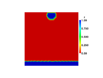
(a) $\hskip 2.84544ptt=0.0\hskip 34.14322pt$

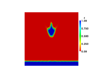
(b) $\hskip 2.84544ptt=(1/4)T$

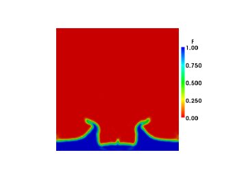
(c) $\hskip 2.84544ptt=(1/2)T$

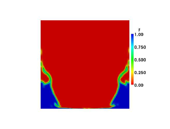
(d) $\hskip 2.84544ptt=(3/4)T\hskip 34.14322pt$

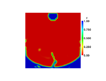
(e) $\hskip 2.84544ptt=T$

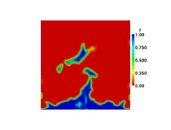
(f) $\hskip 2.84544ptt=(5/4)T$

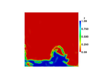
(g) $\hskip 2.84544ptt=(3/2)T\hskip 34.14322pt$

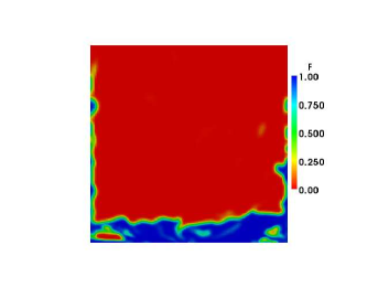
(h) $\hskip 2.84544ptt=(7/4)T$

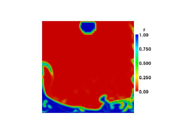
(i) $\hskip 2.84544ptt=2T$

Figure 3: Snapshots of the indicator function $F(t,{\mathbf{x}})$ obtained at the indicated instants of time in the solution of the time–dependent problem (1)–(4) with the parameters $T=1.0$, $V_{d}=1.0$ and $r=0.25$.

IV Algebraic Closure Model

In Section II.2 we introduced the Reynolds decomposition of the flow variables into the time–averaged quantities (denoted with angle brackets $\langle\cdot\rangle$) and fluctuating quantities (denoted with primes). The terms involving averaged products of fluctuating quantities appear as unknowns in averaged equations (22) and must be closed with suitable “closure models”, analogous to those which arise in classical turbulence modeling approaches. The most commonly used methods of turbulence modeling are surveyed in monograph by Popepope . Briefly speaking, depending on their mathematical structure, such approaches fall into two main categories, namely, algebraic models and differential models in which evolution of the quantities introduced to close the system is governed by additional PDEs. Some attempts at deriving closure models for two–phase flows were already made by Brocchini & Peregrine bp01b and by Brocchinib02 who obtained such models for regimes characterized by different values of the turbulent kinetic energy and the turbulent length scale. In this Section, we make an attempt to derive an extremely simple algebraic closure relationship based on an elementary model of the process defined by the following set of assumptions (see also Figure 4).

Assumption 4.

1. Droplets are spherical with radius $r$ and move as rigid objects,

2. there is no collision or coalescence of droplets,

3. droplets are falling periodically with frequency $T^{-1}$ and constant velocity $V_{d}$,

4. the fluid outside droplets (i.e., the gas phase) is motionless,

5. the mean fields do not depend on the vertical coordinate.

We observe that Assumption 4b constrains the problem parameters so that $2r<V_{d}\,T$. It is also to be noted that Assumption 4e implies that the model is effectively one–dimensional with variations only in the direction normal to the effective surface. While the above assumptions are rather far–reaching (in particular, the model does not include any effects of droplet impingement on the free surface), our objective here is to provide some preliminary insights concerning computation of effective free surfaces, and development of closures based on more accurate models is left to future research (some possible directions are discussed briefly in Section VII). We thus proceed to use Assumptions 4 in order to derive expressions for the fluctuating fields $F^{\prime}$, $u^{\prime}$ and $v^{\prime}$ which will be given in terms of the mean fields $\langle F\rangle$ (or ${\tilde{F}}$), $\langle u\rangle$ and $\langle v\rangle$. These expressions will be in turn used to determine the fields $a$ and ${\mathbf{b}}$ in (26e)–(26f).

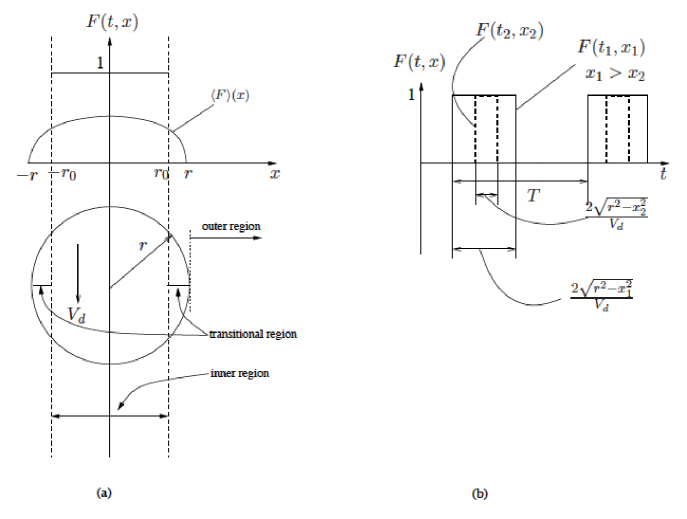
Figure 4: Sketch illustrating the main features of the model based on Assumptions 4: (a) construction of the piecewise–constant approximation ${\tilde{F}}$ to $\langle F\rangle$, (b) time–dependence of the indicator function $F(x,t)$ for different values of the distance $x$.

The coordinate system is shown in Figure 4. We begin by observing that in the model problem considered the horizontal velocity component vanishes identically, i.e., $u(t,x)=0$, $t\geq 0$, $x\in\mathbb{R}$, as do its mean and the corresponding fluctuation fields

$$\langle u\rangle(x)=0,\quad u^{\prime}(t,x)=0,\quad t\geq 0,\ x\in\mathbb{R}.$$ (27)

Since the model considered assumes periodic behavior, without loss of generality we are going to focus on a single period of droplet impingement, i.e., $t\in[0,T]$, and we also remark that the vertical velocity component $v$ and the indicator function $F$ are piecewise–constant functions of time at every point in space. We thus define the following “pulse” function

$$\prod_{\theta}(t)=\left\{\begin{array}[]{ll}1,&\quad 0\leq t\leq\theta\\ 0,&\quad\textrm{otherwise}\end{array}\right.,$$ (28)

where $0\leq\theta<T$, which allows us to write the following expression for the indicator function $F$ as a function of time and the coordinate $x$ (for simplicity, we omit the $y$–dependent phase shift in this expression, as it does not affect the averages which we will ultimately compute)

$$F(t,x)=\left\{\begin{aligned} &\Pi_{\frac{2\sqrt{r^{2}-x^{2}}}{V_{d}}}(t),\quad&&0\leq|x|<r\\ &0,&&|x|\geq r\end{aligned}\right.,$$ (29)

and then the vertical velocity component becomes $v(t,x)=V_{d}\,F(t,x)$ for $t\geq 0$, $x\in\mathbb{R}$. Next, computing the average over one period we obtain

$$\langle F\rangle(x)=\frac{1}{T}\int_{0}^{T}F(t,x)\,dt=\left\{\begin{aligned} &\frac{2\sqrt{r^{2}-x^{2}}}{V_{d}\,T},\quad&&0\leq|x|<r\\ &0,&&|x|\geq r\end{aligned}\right.,$$ (30)

and also have $\langle v\rangle(x)=V_{d}\,\langle F\rangle(x)$. These expressions allow us to evaluate the fluctuating fields as follows

$$v^{\prime}(t,x)=v(t,x)-\langle v\rangle(x) = \left\{\begin{aligned} &V_{d}\,{\Pi}_{\frac{2\sqrt{r^{2}-x^{2}}}{V_{d}}}(t)-\frac{2\sqrt{r^{2}-x^{2}}}{T},\quad&&0\leq|x|<r\\ &0,&&|x|\geq r\end{aligned}\right.,$$ (31)

$$F^{\prime}(t,x)=F(t,x)-\langle F\rangle(x) = \left\{\begin{aligned} &\Pi_{\frac{2\sqrt{r^{2}-x^{2}}}{V_{d}}}(t)-\frac{2\sqrt{r^{2}-x^{2}}}{V_{d}\,T},\quad&&0\leq|x|<r\\ &0,&&|x|\geq r\end{aligned}\right..$$ (32)

We note that for $-r\leq x\leq r$ the averaged indicator function $\langle F\rangle(x)$ has a quadratic distribution which can be interpreted as resulting in a smeared interface. However, in view of Assumption 3, we require a sharp interface $\tilde{\Gamma}_{LG}$ corresponding to a piecewise–constant indicator function ${\tilde{F}}$

$${\tilde{F}}=\left\{\begin{array}[]{ll}1&\quad\mid x\mid\,\leq r_{0}\\ 0&\quad\mid x\mid\,>r_{0}\end{array}\right.,$$ (33)

where $r_{0}$ is the new interface location which can be determined based on the principle of mass conservation. It is expressed using the original smeared (30) and the new piecewise–constant (33) indicator functions as follows

$$\int_{0}^{\infty}\langle F\rangle(x)\,dx=\int_{0}^{\infty}{\tilde{F}}\,dx$$ (34)

from which we obtain

$$r_{0}=\frac{\pi r^{2}}{2V_{d}T}.$$ (35)

In view of Assumption 4b, it is evident that $r_{0}<r$. Therefore, one can recalculate the fluctuating indicator function, now with respect to ${\tilde{F}}$ given by (33) and (35), to obtain

$$F^{\prime}(t,x)=\left\{\begin{array}[]{ll}\Pi_{\frac{2\sqrt{r^{2}-x^{2}}}{V_{d}}}(t)-1&\quad\mid x\mid<r_{0},\\ \Pi_{\frac{2\sqrt{r^{2}-x^{2}}}{V_{d}}}(t)&\quad r_{0}\leq\mid x\mid\leq r,\\ 0&\quad\mid x\mid>r.\end{array}\right.$$ (36)

We remark that the obtained expressions (31) and (32) for the fluctuating quantities depend only on the model parameters $\{T,r,V_{d}\}$ and the position of the effective (sharp) interface $\tilde{\Gamma}_{LG}$. We are thus in the position to calculate the averaged products of fluctuations appearing as components of tensors ${\mathbf{A}}$ and ${\mathbf{B}}$ in (23a) and (23b). First, we observe that in view of (27) we have

$$\langle F^{\prime}u^{\prime}\rangle=\langle F^{\prime}u^{\prime}u^{\prime}\rangle=\langle F^{\prime}u^{\prime}v^{\prime}\rangle=0$$ (37)

everywhere in the domain. As regards the products of fluctuations which do not include $u^{\prime}$, we observe that the form of the expression will depend on the coordinate $x$, and the following three regions are distinguished

1. inner region defined by $\mid x\mid<r_{0}$, i.e., where ${\tilde{F}}(x)=1$ and $\langle F\rangle(x)>0$,

2. transitional region defined by $r_{0}<\mid x\mid<r$, i.e., where ${\tilde{F}}(x)=0$ and $\langle F\rangle(x)>0$,

3. outer region defined by $\mid x\mid>r$, i.e., where ${\tilde{F}}(x)=\langle F\rangle(x)=0$.

The expressions for the averaged products of fluctuating quantities in these regions are discussed in three subsections below, whereas in the last subsection we demonstrate how these expressions can be used to close the terms $a$ and ${\mathbf{b}}$ in boundary conditions (26e)–(26f).

IV.1 Inner Region

In the inner region $|x|<r_{0}$, using (31) and (32), we can write after employing some straightforward properties of pulse function (28)

$$F^{\prime}v^{\prime}=-\frac{2\sqrt{r^{2}-x^{2}}}{T}\Pi_{\frac{2\sqrt{r^{2}-x^{2}}}{V_{d}}}(t)+\frac{2\sqrt{r^{2}-x^{2}}}{T}.$$ (38)

Time–averaging expression (38) we obtain

$$\langle F^{\prime}v^{\prime}\rangle=\frac{2\sqrt{r^{2}-x^{2}}}{T}-\frac{4(x^{2}-r^{2})}{V_{d}\,T^{2}}.$$ (39)

Following the same steps as above, we can deduce that

$$\langle F^{\prime}v^{\prime}v^{\prime}\rangle=\frac{8(r^{2}-x^{2})^{3/2}}{V_{d}\,T^{3}}-\frac{4(r^{2}-x^{2})}{T^{2}}.$$ (40)

IV.2 Transitional Region

In the transitional region $r_{0}<|x|<r$, again using (31) and (32), and following the steps involved in obtaining (39) and (40), we can express $\langle F^{\prime}v^{\prime}\rangle$ and $\langle F^{\prime}v^{\prime}v^{\prime}\rangle$ as

$$\langle F^{\prime}v^{\prime}\rangle =\frac{2\sqrt{r^{2}-x^{2}}}{T}-\frac{4(x^{2}-r^{2})}{V_{d}\,T^{2}},$$ (41a)

$$\langle F^{\prime}v^{\prime}v^{\prime}\rangle =\frac{2V_{d}\sqrt{r^{2}-x^{2}}}{T}-\frac{8(r^{2}-x^{2})}{T^{2}}+\frac{8(r^{2}-x^{2})^{3/2}}{V_{d}\,T^{3}}.$$ (41b)

IV.3 Outer Region

Since in the outer region $|x|>r$ we have $F^{\prime}(x)=0$, it follows that

$$\langle F^{\prime}v^{\prime}\rangle =0,$$ (42a)

$$\langle F^{\prime}v^{\prime}v^{\prime}\rangle =0.$$ (42b)

IV.4 Closure Terms in the Boundary Conditions on the Effective Surface

In this Section we derive expressions for the closure terms $a$ and ${\mathbf{b}}$ in boundary conditions (26e)–(26f) based on the simple algebraic closure model proposed here. First, since $u^{\prime}\equiv 0$ and $\langle u\rangle\equiv 0$, we note that

$${\mathbf{A}}=(\rho_{L}-\rho_{G})\begin{bmatrix}0\\ \langle F^{\prime}v^{\prime}\rangle\\ \end{bmatrix},\qquad{\mathbf{B}}=(\rho_{L}-\rho_{G})\begin{bmatrix}0&0\\ 0&\langle F^{\prime}v^{\prime}v^{\prime}\rangle\\ \end{bmatrix},$$ (43)

where the form of the nonzero entries depends on the location with respect to the effective surface $\tilde{\Gamma}_{LG}$ (see Sections IV.1, IV.2 and IV.3). In our model the location of the effective surface $\tilde{\Gamma}_{LG}$ coincides with the boundary between the inner and transitional regions, cf. Figure 4a. In view of (25) and (43) we therefore have

$$\begin{aligned} a&=(\rho_{L}-\rho_{G})\left(n_{y}\langle F^{\prime}v^{\prime}\rangle\big{|}_{\textrm{transitional}}-n_{y}\langle F^{\prime}v^{\prime}\rangle\big{|}_{\textrm{inner}}\right)=0,\end{aligned}$$ (44)

$$\begin{aligned} {\mathbf{b}}&=(\rho_{L}-\rho_{G})\left(\begin{bmatrix}0\\ n_{y}\langle F^{\prime}v^{\prime}v^{\prime}\rangle\\ \end{bmatrix}\Bigg{|}_{\textrm{transitional}}-\begin{bmatrix}0\\ n_{y}\langle F^{\prime}v^{\prime}v^{\prime}\rangle\\ \end{bmatrix}\Bigg{|}_{\textrm{inner}}\right)\\ &=(\rho_{L}-\rho_{G})\begin{bmatrix}0\\ n_{y}\left[\frac{r}{T^{2}}\sqrt{4V_{d}^{2}T^{2}-\pi^{2}r^{2}}-\frac{r^{2}}{V_{d}^{2}T^{4}}\left(4V_{d}^{2}T^{2}-\pi^{2}r^{2}\right)\right]\end{bmatrix},\end{aligned}$$ (45)

where we also used the relationships derived in Sections IV.1 and IV.2 evaluated at $x=r_{0}$ to express the fluctuating terms. Relations (44) and (45) close our system of averaged equations (26). The conclusion that $a=0$ is consistent with the fact that there is no mass production at the effective surface. It should be emphasized that the proposed closure model is quite problem–specific and it is not obvious whether the same ideas could be used to develop closures for other flows with effective free surfaces. The closure model derived by Brocchini & Peregrine bp01b for an analogous flow regime is more general, and at the same time less explicit, as it is constructed in terms of an a priori unspecified “probability function” describing ejection of droplets with some specific velocity. The model proposed in this Section can be regarded as assuming a specific form of this probability function. A numerical approach well suited for the solution of free–boundary problem (26) is described in the next Section, whereas in Section VI we will analyze the dependence of the solutions on the parameters $\{V_{d},R,T\}$ characterizing the closure model.

V Solution of Averaged Equations with Effective Surfaces Via a Shape Optimization Approach

In Sections II and IV we formulated a set of steady–state PDEs as a simplified time–averaged model of a fluid problem involving unsteady free boundaries such as, for example, the system introduced in Section III with droplets impinging on the pool surface, cf. Figure 1. In the proposed formulation, the steady liquid–gas interface is represented as the effective free surface described mathematically as the discontinuity of the averaged indicator function ${\tilde{F}}$. Therefore, the set of governing equations (26) has the form of a steady free–boundary problem. Since such problems tend to be hard to solve numerically, we argue below that a computationally efficient approach can be developed by formulating this problem in terms of shape optimization. More specifically, we will frame it as finding an optimal shape of the interface (i.e., effective free boundary $\tilde{\Gamma}_{LG}$) such that a cost functional representing the residual of one of the interface boundary conditions will be minimized with respect to the position of the interface subject to the constraints representing the governing (time–averaged) equations and the remaining boundary conditions. We refer the reader to the monograph by Neittaanmaki et al.nst06 for a general discussion of advantages of such an approach, and to papers by Volkov & Protas vp08a and Volkov et al. vplg09a for a discussion of some applications to problems similar to the one studied here which also included treatment of contact lines.

System (26) represents a steady–state free–boundary problem where $\tilde{\Gamma}_{LG}$ has to be found as a part of the solution. By fixing the domain and its boundary $\tilde{\Gamma}_{LG}$, and removing one of the boundary conditions, for example, the normal component of (26f), we obtain a steady fixed–boundary problem. The residual of the normal component of condition (26f) is then minimized with respect to the unknown shape of the effective surface $\tilde{\Gamma}_{LG}$ using a suitable shape–optimization algorithm. The choice of the normal component of condition (26f) as the optimization criterion is motivated by the fact that this condition contains closure terms, hence in practical situations need not be satisfied up to the machine accuracy.

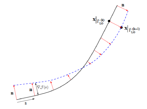
Figure 5: Schematic of a single step of the shape optimization algorithm (50): (solid line) approximation to the effective surface at the $k$–th iteration and (dashed line) approximation to the effective surface at the $k+1$–th iteration.

Our solution approach is then formulated as follows. Suppose we define the function $\chi\;:\;\tilde{\Gamma}_{LG}\rightarrow\mathbb{R}$ which will represent the residual of the normal component of the momentum boundary condition (26f)

$$\chi\triangleq{\mathbf{n}}\cdot\langle\boldsymbol{\sigma}_{L}^{\mu}\rangle\cdot{\mathbf{n}}-{\mathbf{n}}\cdot\langle\boldsymbol{\sigma}_{G}^{\mu}\rangle\cdot{\mathbf{n}}-\gamma\kappa\,-\mathbf{b}\cdot{\mathbf{n}}.$$ (46)

The cost functional can then be defined as

$$\mathcal{J}(\tilde{\Gamma}_{LG})=\frac{1}{2}\int_{\tilde{\Gamma}_{LG}}\chi^{2}\,d\sigma,$$ (47)

so that the optimization problem becomes

$$\min_{\tilde{\Gamma}_{LG}}\mathcal{J}(\tilde{\Gamma}_{LG}),$$ (48)

where $\chi$ in (46) depends on the shape of the effective free surface $\tilde{\Gamma}_{LG}$, which is the control variable in optimization problem (48), via governing PDEs (26a)–(26d) subject to boundary conditions (26e), (26g), and the tangential component of condition (26f), i.e.,

$$\mathbf{t}\cdot\Big{[}\langle\boldsymbol{\sigma}\rangle\Big{]}_{L}^{G}\cdot{\mathbf{n}}=0,\quad\textrm{on}\quad\tilde{\Gamma}_{LG}.$$ (49)

Thus, we observe that the system of PDEs serving as the constraint for optimization problem (48) has in fact the form of a fixed–boundary problem which makes evaluation of the cost functional at every iteration easier (i.e., it corresponds to the approximation $\tilde{\Gamma}_{LG}^{\,(k)}$ of the effective surface at the given $k$–th iteration). The position of the effective interface $\tilde{\Gamma}_{LG}$ can then be found using the following iterative gradient–descent algorithm

$${\mathbf{x}}|_{\tilde{\Gamma}_{LG}^{\,(k+1)}}={\mathbf{x}}|_{\tilde{\Gamma}_{LG}^{\,(k)}}+\tau_{k}\,{\mathbf{G}}\left[\nabla{\mathcal{J}}\left(\tilde{\Gamma}_{LG}^{\,(k)}\right)\,{\mathbf{n}}\right],\qquad k=1,2,\dots,$$ (50)

where ${\mathbf{x}}|_{\tilde{\Gamma}_{LG}^{\,(k)}}\in\mathbb{R}^{2}$ represents points on the interface $\tilde{\Gamma}_{LG}$ at the $k$–th iteration and $\tau_{k}$ is the length of the step in the descent direction. The function ${\mathbf{G}}$ determines the specific form of the optimization algorithm used (e.g., the steepest descent, conjugate gradients, or quasi–Newton method, etc., see Ref. nw00, ). In our results reported in Section VI we use the Conjugate Gradients Method. A central element of algorithm (50) is the cost functional gradient $\nabla{\mathcal{J}}\,:\,\tilde{\Gamma}_{LG}^{(k)}\rightarrow\mathbb{R}$ representing the continuous sensitivity of cost functional (47) to infinitesimal modifications in the normal direction of the shape of $\tilde{\Gamma}^{(k)}_{LG}$. In other words, as indicated in Figure 5, the scalar–valued function $\nabla{\mathcal{J}}\left(\tilde{\Gamma}_{LG}^{(k)}\right)$, depending on the arclength coordinate along the interface, represents the normal displacement of the current approximation to the effective surface $\tilde{\Gamma}^{(k)}_{LG}$ resulting in the largest possible decrease of cost functional (47), see also Appendix A.2. The contact points, where the effective surface $\tilde{\Gamma}_{LG}$ meets the solid boundary $\Gamma_{0}$, require special attention and we follow here the approach developed by Volkov and Protasvp08a to deal with the contact line problems in the context of shape optimization. Determination of the gradient $\nabla{\mathcal{J}}$ requires the solution of a suitably–defined adjoint system and details concerning its derivation are deferred to Appendix A. The step size $\tau_{k}$ is obtained via solution of the following line minimization problem

$$\tau_{k}=\operatorname{argmin}_{\tau>0}{\mathcal{J}}\left({\mathbf{x}}|_{\tilde{\Gamma}_{LG}^{\,(k)}}+\tau\,{\mathbf{G}}\left[\nabla{\mathcal{J}}\left(\tilde{\Gamma}_{LG}^{\,(k)}\right)\,{\mathbf{n}}\right]\right)$$ (51)

which can be done, for example, using Brent’s method, see Ref. nw00, . The complete approach is summarized in Algorithm 1.

  ALGORITHM 1: Iterative minimization algorithm for solving system (26) via a shape optimization approach.

Input: $\epsilon_{\tau}$ (adjustable tolerance), $\tilde{\Gamma}_{LG}^{(0)}$ (initial guess for the effective surface)

Output: $\tilde{\Gamma}_{LG}$ (effective surface)

 

  $n\leftarrow 0$

  $\tilde{\Gamma}_{LG}^{(0)}\leftarrow$ initial guess (Figure 6)

  repeat

     solve direct system

     solve adjoint system

     compute gradient $\nabla\mathcal{J}\left(\tilde{\Gamma}_{LG}^{\,(n)}\right)$

     perform line minimization to determine $\tau^{(n)}$

     update effective surface using (50)

     $n\leftarrow n+1$;

  until $\tau^{(n)}<\epsilon_{\tau}$.

 

Our time–dependent model problem (1)–(4) is set up such that the mass of liquid remains constant over every period of droplet impingement (the amount of mass drained at the bottom of the container equals the mass added in the form of droplets at the top of the domain, cf. Section III). Therefore, it is necessary to ensure that in our steady–state averaged problem with effective surfaces (26) the same mass is enclosed in the liquid domain $\tilde{\Omega}_{L}$. Mathematically, this is implemented by constructing an initial guess for the liquid domain $\tilde{\Omega}_{L}^{(0)}$ which has the prescribed mass and then making sure that this mass is not changed at subsequent iterations. For this to happen, it is required that the shape gradients $\nabla\mathcal{J}(\tilde{\Gamma}_{LG})$ do not change the volume of $\tilde{\Omega}_{L}$. This property is enforced at each iteration as follows. First, we calculate the mean value $M\in\mathbb{R}$ of the gradient on the effective surface

$$M=\frac{1}{L}\,\int_{0}^{L}\nabla\mathcal{J}(s)ds$$ (52)

where $s\in[0,L]$ is the corresponding arclength coordinate. The new gradient with zero mean displacement in the normal direction is then obtained as

$$\widetilde{\nabla\mathcal{J}}(s)=\nabla\mathcal{J}(s)-M,\qquad\forall_{s\in[0,L]}.$$ (53)

The cost functional gradient $\nabla\mathcal{J}$ is replaced with zero–mean gradient $\widetilde{\nabla\mathcal{J}}$ in expressions (50) and (51).

VI Results and Discussions

In this Section we present sample computations for the problem of determining the effective free surfaces in the flow described in Section III, see also Figure 1. In order to calculate the cost functional gradient (given by expression (72) in Appendix A) we need to solve “direct” system (26) and adjoint system (67)–(68). Both these solutions are obtained using the finite–element method implemented in the COMSOL script environment. The domain (Figure 6) is discretized using approximately 4000 Lagrangian elements with mesh size varying between 0.9 to 0.01. In all computations presented here we used the physical parameters with values indicated in Table 1 and these calculations were performed using the Navier–Stokes and Poisson solvers available in COMSOL. For illustration purposes, in Figures 7a and 7b we show the fields of the direct and adjoint vorticity obtained at the first iteration. Before analyzing the solutions with effective free surfaces obtained for different parameters of the closure models, we validate the calculation of the cost functional gradient which is the main element of our computational approach, cf. Section V and Appendix A.

Physical Parameter	Value
Density of the liquid, $\rho_{L}$	$1000[Kg.m^{-3}]$
Dynamic viscosity of the liquid, $\mu_{L}$	0.001$[Pa.s]$
Density of the gas, $\rho_{G}$	$1[Kg.m^{-3}]$
Dynamic viscosity of the gas, $\mu_{G}$	0.00001$[Pa.s]$
Gravitational acceleration, ${\mathbf{g}}$	$9.81[m.s^{-2}]$
Surface tension, $\gamma$	$0.7[N.m^{-1}]$

Table 1: Values of the physical parameters used in the computation.

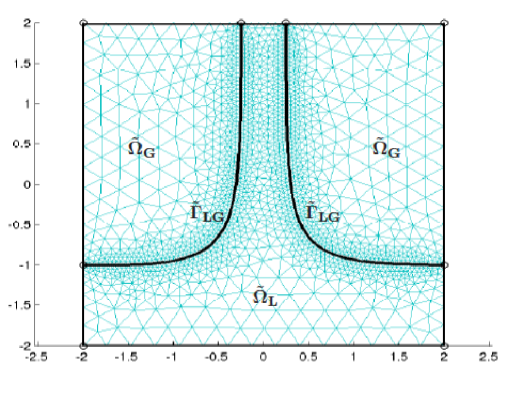
Figure 6: Geometry of the computational domain $\Omega$ with the liquid and gas subdomains $\tilde{\Omega}_{L}$ and $\tilde{\Omega}_{G}$ and the effective boundary $\tilde{\Gamma}_{LG}$ used as the initial guess in shape optimization algorithm (50). The figure also shows the unstructured triangular finite–element mesh used in the solution of direct and adjoint problems.

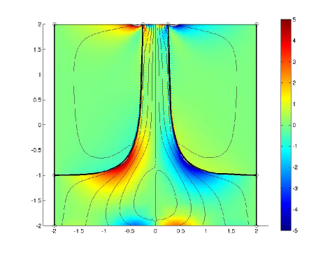
(a)

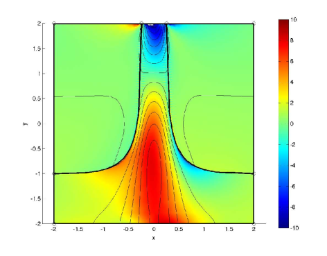
Figure 7: Vorticity fields and streamlines in the numerical solution of (a) direct problem and (b) adjoint problem at the first iteration.

VI.1 Validation of the Shape Optimization Approach

In this Section we demonstrate the consistency of the gradients $\nabla_{\tilde{\Gamma}_{LG}}\mathcal{J}$ obtained using expression (72) in Appendix A.3. A standard test consists in computing the Gâteaux differential of cost functional $\mathcal{J}(\tilde{\Gamma}_{LG})$ in some arbitrary direction ${\mathbf{x}}^{\prime}=\zeta^{\prime}{\mathbf{n}}$ using a finite–difference technique and comparing it with the expressions for the same differential obtained using the gradient $\nabla_{\tilde{\Gamma}_{LG}}\mathcal{J}$ and Riesz representation formula (61). The ratio of these two expressions, which is a function of the finite–difference step size $\epsilon$, is defined as

$$\varkappa_{\tilde{\Gamma}_{LG}}(\epsilon)\triangleq\frac{\mathcal{J}({\mathbf{x}}_{\tilde{\Gamma}_{LG}}+\epsilon\zeta^{\prime}{\mathbf{n}})-\mathcal{J}(\tilde{\Gamma}_{LG})}{\epsilon\big{\langle}\nabla_{\tilde{\Gamma}_{LG}}\mathcal{J},\zeta^{\prime}\big{\rangle}}.$$ (54)

Proximity of $\varkappa_{\tilde{\Gamma}_{LG}}(\epsilon)$ to the unity is thus a measure of the accuracy of the cost functional gradient computed based on the adjoint field. Figure 9 shows the behavior of the quantity $\varkappa_{\tilde{\Gamma}_{LG}}$ as a function of the parameter $\epsilon$ for different perturbations $\zeta^{\prime}$. We note that in all cases the quantity $\varkappa_{\tilde{\Gamma}_{LG}}(\epsilon)$ is quite close to unity for $\epsilon$ spanning over 5 orders of magnitude which indicates that our gradients are evaluated fairly accurately. Figure 9 reveals deviations of $\varkappa_{\tilde{\Gamma}_{LG}}(\epsilon)$ from unity for large values of $\epsilon$, which is due to truncation errors, and also for very small $\epsilon$, due to round–off errors, both of which are well–known effects. These inaccuracies do not affect the optimization process, since the deviations observed for very small $\epsilon$ are only an artifact of how expression (54) is evaluated, whereas large values of $\epsilon$ (or, equivalently, $\tau$) are outside the range of validity of the linearization on which the optimization approach is based. We also performed a grid–refinement study of the cost functional gradients which indicated that the calculation of the gradients is not sensitive to the resolution. Figure 9 shows the decrease of cost functional (47) in the case with and without the closure terms $a$ and ${\mathbf{b}}$ in boundary conditions (26e)–(26f) as a function of the number of iterations. We observe that the proposed algorithm results in a steady convergence despite the complicated nature of the problem, although the rate of convergence is relatively slow, especially in the case when the closure model is present.

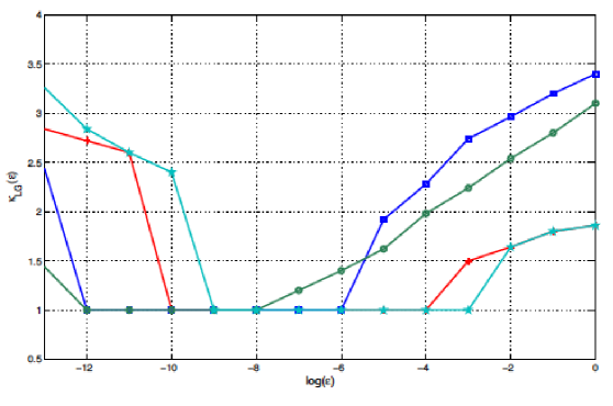
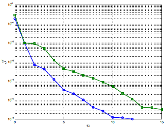
Figure 8: The diagnostic quantity $\varkappa_{\Gamma_{LG}}(\epsilon)$ as a function of $\epsilon$ for different perturbations ($\star$) $\zeta^{\prime}(s)=\sin(2\pi s/L)$, ($\circ$) $\zeta^{\prime}(s)=\sin(2\pi s/L)$, ($\ast$) $\zeta^{\prime}(s)=\arcsin(2s/L-1)$, ($\Box$) $\zeta^{\prime}(s)=\arccos(2s/L-1)$, where $0\leq s\leq L$.

Figure 9: Cost functional ${\mathcal{J}}(\tilde{\Gamma}_{LG}^{(n)})$ as a function of the iteration count $n$ for ($\bullet$) the case without closure terms and ($\blacksquare$) the case with closure terms $a$ and ${\mathbf{b}}$ in boundary conditions (26e)–(26f). The values of the problem parameters are $V_{d}=1.0$, $r=0.25$, and $T=3$.

VI.2 Effective Surfaces for Different Parameters in the Closure Model

In this Section we employ the computational approach developed in Section V and validated in Section VI.1 to construct effective surfaces corresponding to different values of the three parameters $\{V_{d},r,T\}$ characterizing the algebraic closure model introduced in Section IV. In order to reveal different trends, in Figures 10a,b,c we show the effective surfaces obtained by changing one parameter with the other two held fixed. For comparison, in these Figures we also include the effective surfaces obtained without any closure model (i.e., with ${\mathbf{b}}={\mathbf{0}}$ in (26f)). The parameters are chosen in such a way that the case with $\{V_{d}=1.0,r=0.25,T=3\}$ is present in all three Figures 10a,b,c where it represents the intermediate solution. First of all, we observe that in all cases smooth effective surfaces have been obtained. As regards the results shown in Figures 10a and 10b, we observe that the effective surfaces approach the effective surface obtained in the case with no closure as $r\rightarrow 0$ and $T\rightarrow\infty$, respectively. This is consistent with the fact that $\lim_{r\rightarrow 0}{\mathbf{b}}={\mathbf{0}}$ with $V_{d}$ and $T$ fixed, and $\lim_{T\rightarrow\infty}{\mathbf{b}}={\mathbf{0}}$ with $V_{d}$ and $r$ fixed, cf. (45). In the other limits, i.e., for large $r$ (Figure 10a) and small $T$ (Figure 10b), we observe that the liquid column $\tilde{\Omega}_{L}$ becomes much thinner. As regards the dependence on droplet velocity $V_{d}$, from (45) we observe that $V_{d}=\frac{\pi r}{2T}<\frac{2r}{T}$ would correspond to the case with a vanishing closure model (i.e., ${\mathbf{b}}={\mathbf{0}}$), however, this value of $V_{d}$ is outside the range of parameter values consistent with Assumption 4b. Hence, convergence of effective surfaces to the surface corresponding to the case with no closure is not observed in Figure 10c. We observe that in the proposed model the closure terms contribute additional flux of momentum in the direction tangential to the effective surface which can be interpreted as additional shear stress, cf. (26f) and (45). In the cases with large $r$ and small $T$, corresponding to a thinner liquid column $\tilde{\Omega}_{L}$, the effect of the closure model could be compared to an increase of the surface tension (although this analogy is rather superficial, since the surface tension contributes to the normal stresses). We also add that, in addition to the effective surfaces presented in Figures 10a,b,c, for some parameter values we also found solutions featuring asymmetric effective surfaces. This nonuniqueness of solutions is a consequence of the nonlinearity of the governing system which is reflected in the nonconvexity of optimization problem (48). Since these asymmetric solutions are not physically relevant, at least not from the point of view of the actual applications of interest to us, we do not discuss them in this work. In problems with multiple solutions in which such selection cannot be done based on the properties of symmetry, one can identify the relevant solution as the one corresponding to the smallest value of cost functional ${\mathcal{J}}(\tilde{\Gamma}_{LG})$ reflecting the smallest residual (46).

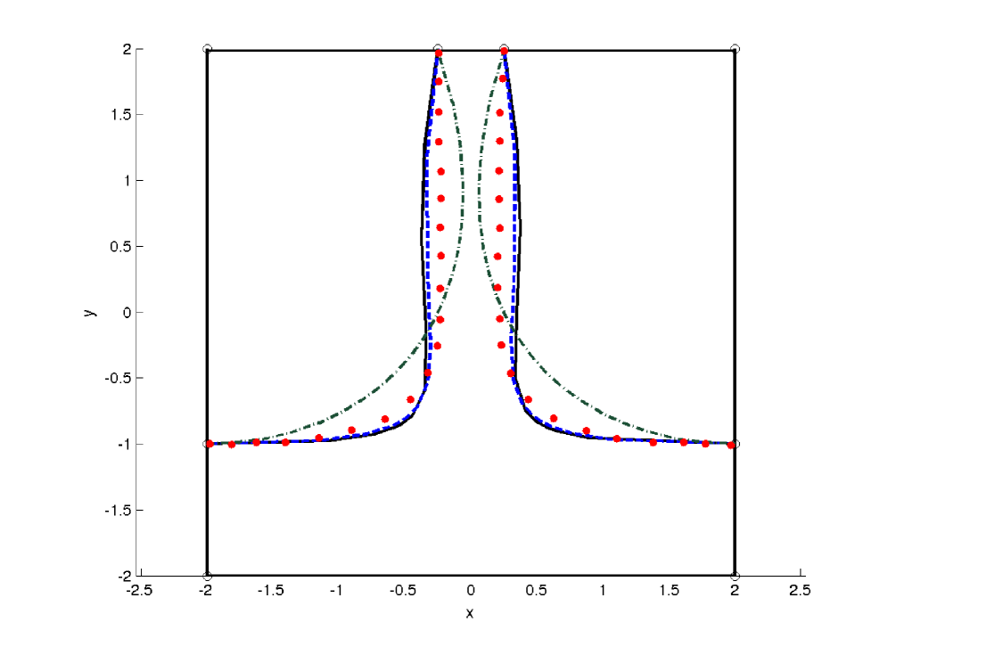
’—–’ No closure, ’ - - - ’ $r=0.1$,

’$\cdots$’, $r=0.25$, ’$-\cdot-\cdot$’, $r=0.5$

with $V_{d}=1.0$ and $T=3$

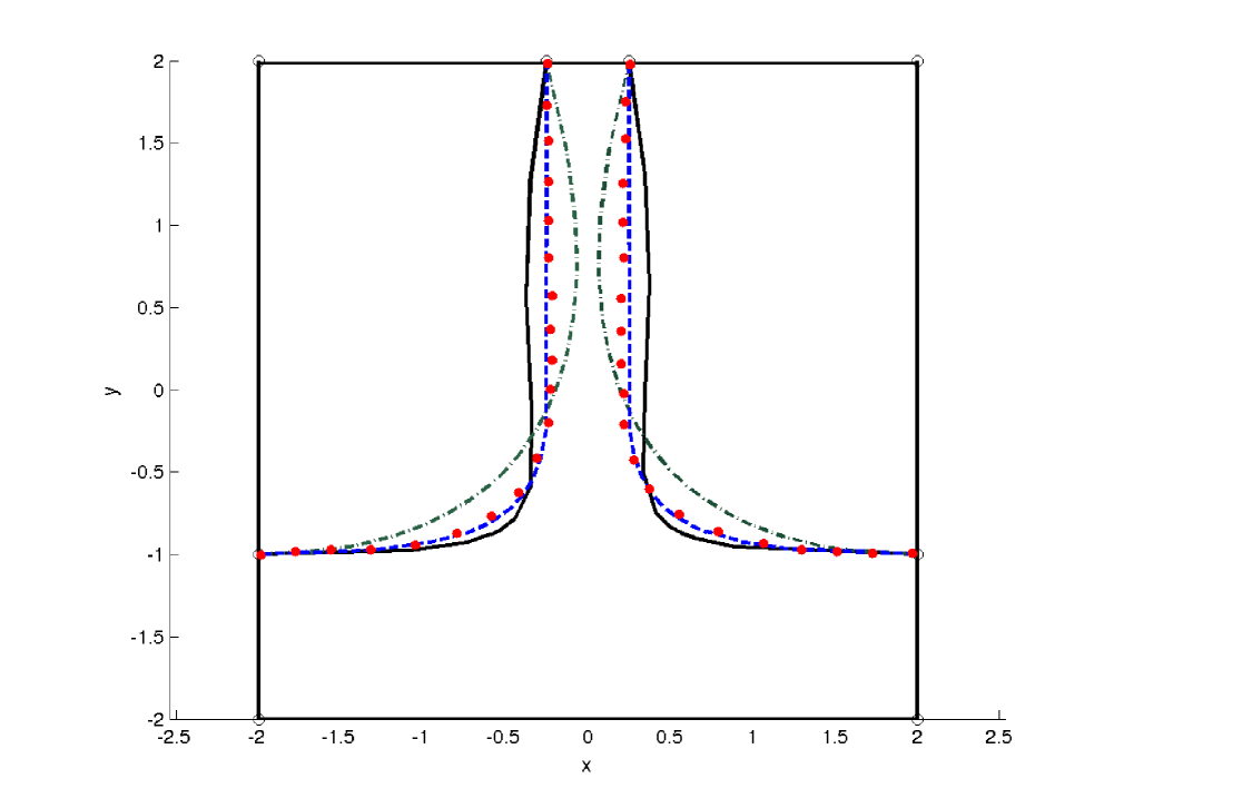
’—–’ No closure, ’$-\cdot-\cdot$’, $T=1$,

’$\cdots$’, $T=3$, ’ - - - ’ $T=6$’,

with $V_{d}=1.0$ and $r=0.25$

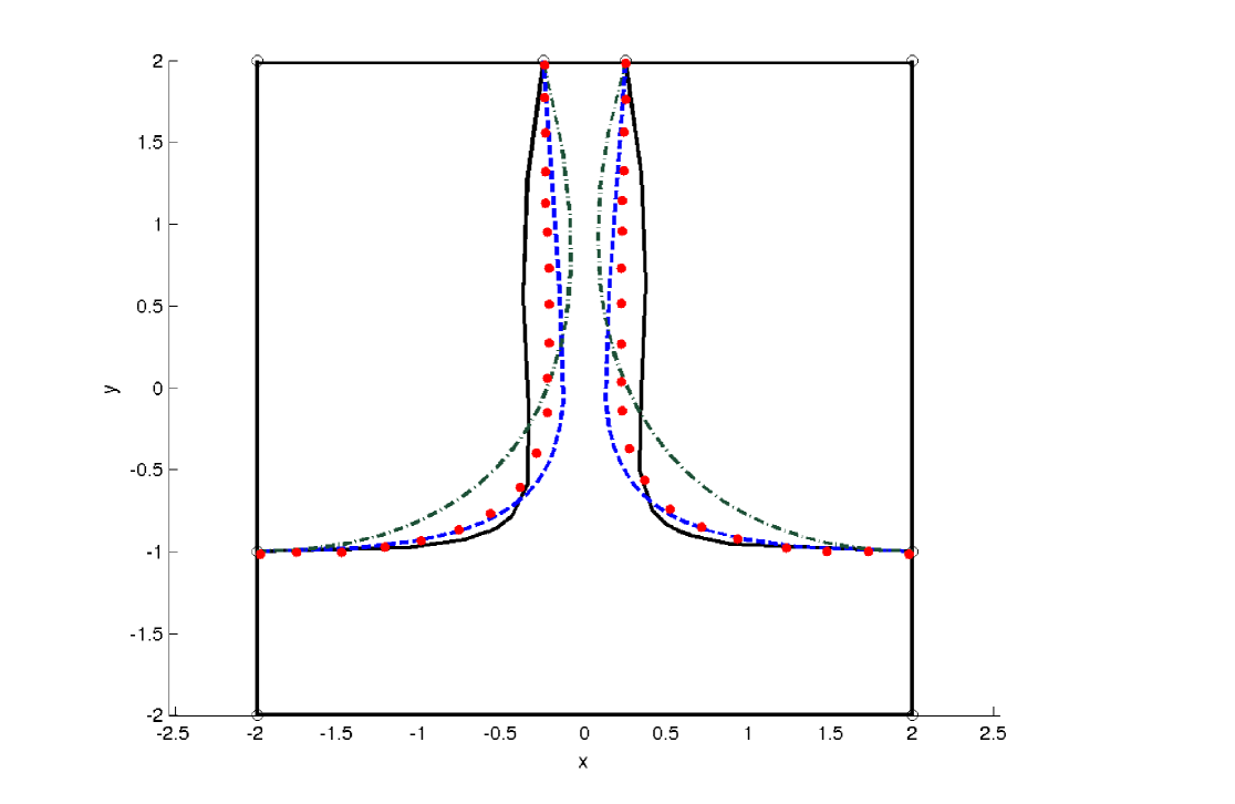
’—–’ No closure, ’ $-\cdot-\cdot$ ’ $V_{d}=0.5$,

’$\cdots$’ $V_{d}=1.0$, ’ - - - ’ $V_{d}=1.25$,

with $r=0.25$ and $T=3$

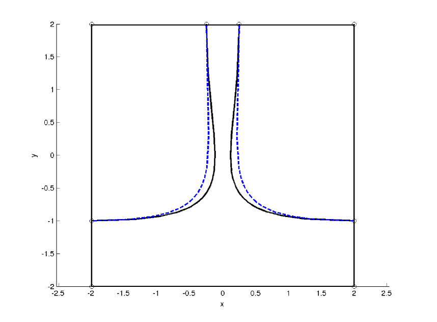
’—–’ data from the unsteady problem

(see Figure 11),

’$---$’ algebraic model from Section IV

Figure 10: Dependence of the shape of the effective surface $\tilde{\Gamma}_{LG}$ on the parameters of the algebraic closure model introduced in Section IV: (a) droplet radius $r$, (b) frequency $T^{-1}$ of droplet impingement, and (c) droplet velocity $V_{d}$ with other parameters held fixed (see captions of individual subfigures); Figure (d) shows the comparison of the effective free surfaces $\tilde{\Gamma}_{LG}$ obtained using the algebraic closure model from Section IV and the approach described in Section VI.2 in which terms $a$ and ${\mathbf{b}}$ are evaluated based on the actual data obtained from the time–dependent flow problem with the parameter values $V_{d}=1.0$, $r=0.25$ and $T=3$.

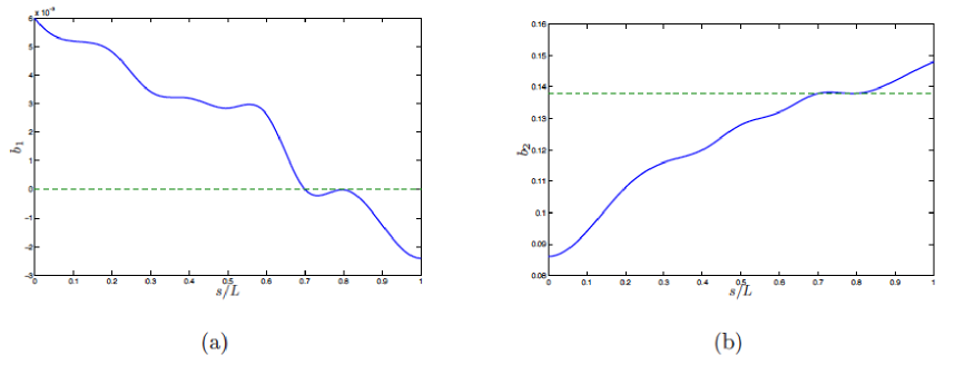
Figure 11: Comparison of the terms (a) $b_{1}$ and (b) $b_{2}$, cf. (25), evaluated based on (solid line) the averaged solution of the time–dependent problem and (dashed line) the closure model described in Section IV, cf. (45). The data is shown as a function of the normalized arclength coordinate $s/L$ along the effective surface $\tilde{\Gamma}_{LG}$ measured from the top, and the values of the parameters are $V_{d}=1.0$, $r=0.25$ and $T=3$.

Finally, in Figure 10d, we perform a comparison between the effective free surfaces constructed using the algebraic closure model from Section IV and using the time–averaged solutions of the original unsteady problem to evaluate the terms $a$ and ${\mathbf{b}}$ via relations (23) and (25). The parameters used in this case are $V_{d}=1.0$, $r=0.25$ and $T=3.0$, and the corresponding data for ${\mathbf{b}}$ obtained by averaging over 200 periods of droplet impingement in the time–dependent case is shown in Figure 11 (the data for the term $a$ is not shown as it vanishes by construction in both cases, cf. (44)). For comparison, in Figure 11 we also indicate the values of the components of ${\mathbf{b}}$ obtained from expressions (23), and we see that the predictions of the simple algebraic closure model developed in Section IV are not too far off from the actual data: as regards the vertical component $b_{2}$, they are within the same order of magnitude (Figure 11b), whereas for the horizontal component $b_{1}$ the difference is ${\mathcal{O}}(10^{-3})$ (Figure 11a). We add that for both $b_{1}$ and $b_{2}$ there exists a part of the effective surface $\tilde{\Gamma}_{LG}$, located towards the bottom of the liquid column $\tilde{\Omega}_{L}$, where the agreement between the closure model and the actual data is particularly good. In Figure 10d we note an overall fairly good agreement between the effective surfaces obtained with terms $a$ and ${\mathbf{b}}$ evaluated in the two different ways. This is, in particular, the case as regards the top part of the liquid column $\tilde{\Omega}_{L}$ which, somewhat interestingly, does not coincide with the region where the closure model is the most accurate according to the data from Figure 11. We attribute this effect to the nonlinear and nonlocal character of the averaged free–boundary problem (26). Finally, we conclude that, despite its simplicity, our closure model performs relatively well in the present problem.

VII Conclusions

In this investigation we revisited the concept of “effective free surfaces” arising in the solution of time–averaged hydrodynamic equations in the presence of free boundaries hw00 ; bp01a ; bp01b ; wo11 . The novelty of our work consists in formulating the problem such that there is a sharp interface separating the two phases in the time–averaged sense, an approach which appears preferable from the point of view of a number of possible applications. The resulting system of equations is of the free–boundary type and we also propose a flexible and efficient numerical method for the solution of this problem which is based on the shape–optimization formulation. Subject to some clearly stated assumptions, the terms representing the average effect of the boundary fluctuations appear in the form of interface boundary conditions, and a simple algebraic model is proposed to close these terms (this is to be contrasted with the “classical” Reynolds stresses which are defined in the bulk of the flow).

This work is motivated by applications of optimization and optimal control theory to problems involving free surfaces. In such problems dealing with time–dependent governing equations leads to technical difficulties, many of which are mitigated when methods of optimization are applied to a steady problem with effective free surfaces. The model problem considered in this study concerns impingement of free–falling droplets on a liquid with a free surface in two dimensions and is motivated by optimization of the mass and momentum transfer phenomena in certain advanced welding processes, see Volkov et al.vplg09a . The computational results shown in this paper are, to the best of our knowledge, the first ever presented for a problem of this type where the effective boundary has the form of a sharp interface. The computed effective free surfaces exhibit a consistent dependence on the problem parameters introduced via the closure model, and despite the admitted simplicity of this model, these results match well the effective surfaces obtained using data from the solution of the time–dependent problem.

A key element of the proposed approach is a closure model for the fluctuation terms representing the motion of the free surfaces. The model we developed here is a very elementary one resulting in simple algebraic relationships. As in the traditional turbulence researchpope , more advanced and more general closure models can be derived based on the PDEs describing the transport of various relevant quantities such as the turbulent kinetic energy, the turbulent length scale, etc. In fact, such approaches have already been explored in the context of free–boundary problemsbp01b ; b02 leading to more general, albeit less explicit, closure models than the model considered here.

In addition to investigating such more advanced closure models, our future work will focus on quantifying the effect of and, ultimately, weakening the assumptions employed to derive the present approach, so that it can be applied to a broader class of problems, especially interfacial. At the same time, we will seek to incorporate this approach into the optimization–oriented models of complex thermo–fluid phenomena occurring in welding processes, such as discussed in Volkov et. alvplg09a . While the present investigation responded to needs arising from a certain class of applications, it has also highlighted a number of more fundamental research questions which it will be worthwhile to explore based on even simpler model problems such as, e.g., capillary or gravity waves on a flat interface.

Appendix A Characterization of Cost Functional Gradients in Effective Surface Calculations

In this Appendix we obtain expressions for the gradient $\boldsymbol{\nabla}_{\tilde{\Gamma}_{LG}}{\mathcal{J}}$ of the cost functional (47) with respect to the position of the effective interface $\tilde{\Gamma}_{LG}$. Characterization of this gradient requires one to differentiate solutions of governing PDEs system (26) with respect to the shape of the domain on which these solutions are defined. This is done properly using tools of the shape–differential calculus sz92 ; dz01a which are briefly introduced below. In the calculations we will assume that the problem parameters $\{V_{d},r,T\}$ are given. Hereafter primes (^′) will denote perturbations (shape differentials) of the different variables which is consistent with the convention used in the literaturedz01a . Since fluctuation variables do not appear in this Appendix, there is no risk of confusion resulting from this abuse of notation.

A.1 Shape Calculus

In the shape calculus perturbations of the interface geometry can be represented as

$${\mathbf{x}}(\eta,{\mathbf{x}}^{\prime})={\mathbf{x}}+\eta{\mathbf{x}}^{\prime}\quad\text{for}\quad{\mathbf{x}}\in\tilde{\Gamma}_{LG}(0),$$ (55)

where $\eta$ is a real parameter, $\tilde{\Gamma}_{LG}(0)$ is the original unperturbed boundary and ${\mathbf{x}}^{\prime}:\Omega\to\mathbb{R}^{2}$ is a “velocity” field characterizing the perturbation. The Gâteaux shape differential of a functional such as (46) with respect to the shape of the interface $\tilde{\Gamma}_{LG}$ and computed in the direction of perturbation field ${\mathbf{x}}^{\prime}$ is given by

$$\mathcal{J}^{\prime}(\tilde{\Gamma}_{LG};{\mathbf{x}}^{\prime})=\lim_{\eta\to 0}\frac{\mathcal{J}({\mathbf{x}}_{\tilde{\Gamma}_{LG}}+\eta{\mathbf{x}}^{\prime})-\mathcal{J}({\mathbf{x}}_{\tilde{\Gamma}_{LG}})}{\eta}.$$ (56)

In the sequel we will need the following fundamental result concerning shape–differentiation of functionals defined on smooth domains $\Omega(\eta,{\mathbf{x}}^{\prime})$ and on their boundaries, and involving smooth functions $f$ and $g$ as integrands dz01a

$$\Bigg{(}\int_{\Omega(\eta,{\mathbf{x}}^{\prime})}f\,d\Omega+\int_{\partial\Omega(\eta,{\mathbf{x}}^{\prime})}g\,d\sigma\Bigg{)}^{\prime}= \int_{\Omega(0)}f^{\prime}\,d\Omega+\int_{\partial\Omega(0)}g^{\prime}\,d\sigma+$$ (57)

$$\int_{\partial\Omega(0)}\left(f+\kappa\,g+\frac{\partial g}{\partial n}\right)({\mathbf{x}}^{\prime}\cdot{\mathbf{n}})\,d\sigma,$$

where $f^{\prime}$ and $g^{\prime}$ are the shape derivatives of $f$ and $g$, and $\kappa$ is the curvature of the boundary $\partial\Omega(0)$.

A.2 Differential of Cost Functional

In order to obtain the gradients $\nabla_{\tilde{\Gamma}_{LG}}\mathcal{J}$ of the cost functional (47) with respect to the control variable $\tilde{\Gamma}_{LG}$, we first need to obtain the Gâteaux (directional) derivative of ${\mathcal{J}}(\tilde{\Gamma}_{LG})$. Using relation (57) and substituting $f\equiv 0$ and $g=\frac{1}{2}\chi^{2}$, we obtain the following expression for the cost functional differential

$$\mathcal{J}^{\prime}(\Gamma;{\mathbf{x}}^{\prime})=\int_{\Gamma}\chi\,\chi^{\prime}\,d\sigma+\int_{\tilde{\Gamma}_{LG}}\left(\frac{1}{2}\kappa\,\chi^{2}+\chi\,\frac{\partial\chi}{\partial n}\right)({\mathbf{x}}^{\prime}\cdot{\mathbf{n}})\,d\sigma,$$ (58)

where

$$\chi^{\prime}={\mathbf{n}}^{\prime}\cdot\langle\boldsymbol{\sigma}_{L}^{\mu}\rangle\cdot{\mathbf{n}}+{\mathbf{n}}\cdot\langle\boldsymbol{\sigma}_{L}^{\mu}\rangle^{\prime}\cdot{\mathbf{n}}+{\mathbf{n}}\cdot\langle\boldsymbol{\sigma}_{L}^{\mu}\rangle\cdot{\mathbf{n}}^{\prime}-{\mathbf{n}}^{\prime}\cdot\langle\boldsymbol{\sigma}_{G}^{\mu}\rangle\cdot{\mathbf{n}}-{\mathbf{n}}\cdot\langle\boldsymbol{\sigma}_{G}^{\mu}\rangle^{\prime}\cdot{\mathbf{n}}-{\mathbf{n}}\cdot\langle\boldsymbol{\sigma}_{G}^{\mu}\rangle\cdot{\mathbf{n}}^{\prime}\\ -\kappa^{\prime}\,\gamma-2(\rho_{L}-\rho_{G})\left[\frac{r}{T^{2}}\sqrt{4V_{d}^{2}T^{2}-\pi^{2}r^{2}}-\frac{r^{2}}{V_{d}^{2}T^{4}}\left(4V_{d}^{2}T^{2}-\pi^{2}r^{2}\right)\right](\mathbf{e_{y}}\cdot{\mathbf{n}})(\mathbf{e_{y}}\cdot{\mathbf{n}}^{\prime}).$$ (59)

Using the following identities of shape calculus dz01a ${\mathbf{n}}^{\prime}=-\boldsymbol{\nabla}_{\Gamma}({\mathbf{x}}^{\prime}\cdot{\mathbf{n}})$ and $\kappa^{\prime}=-\Delta_{\Gamma}({\mathbf{x}}^{\prime}\cdot{\mathbf{n}})$, where $\boldsymbol{\nabla}_{\Gamma}$ and $\Delta_{\Gamma}$ are the tangential gradient and the Laplace–Beltrami operator, we obtain

$$\mathcal{J}^{\prime}(\Gamma;{\mathbf{x}}^{\prime})=\int_{\tilde{\Gamma}_{LG}}\Bigg{[}\chi\,\Bigg{(}\big{[}{\mathbf{n}}\cdot\boldsymbol{\sigma}^{\prime}\cdot{\mathbf{n}}\big{]}_{L}^{G}-2\boldsymbol{\nabla}_{\Gamma}({\mathbf{x}}^{\prime}\cdot{\mathbf{n}})\cdot\langle\boldsymbol{\sigma}_{L}^{\mu}\rangle\cdot{\mathbf{n}}+2\boldsymbol{\nabla}_{\Gamma}({\mathbf{x}}^{\prime}\cdot{\mathbf{n}})\cdot\langle\boldsymbol{\sigma}_{G}^{\mu}\rangle\cdot{\mathbf{n}}+\gamma\Delta_{\Gamma}({\mathbf{x}}^{\prime}\cdot{\mathbf{n}})\Bigg{)}\\ +2(\rho_{L}-\rho_{G})\left[\frac{r}{T^{2}}\sqrt{4V_{d}^{2}T^{2}-\pi^{2}r^{2}}-\frac{r^{2}}{V_{d}^{2}T^{4}}\left(4V_{d}^{2}T^{2}-\pi^{2}r^{2}\right)\right](\mathbf{e_{y}}\cdot{\mathbf{n}})\left(\mathbf{e_{y}}\cdot\boldsymbol{\nabla}_{\Gamma}({\mathbf{x}}^{\prime}\cdot{\mathbf{n}})\right)\\ +\left(\frac{1}{2}\kappa\,\chi^{2}+\chi\,\frac{\partial\chi}{\partial n}\right)({\mathbf{x}}^{\prime}\cdot{\mathbf{n}})\Bigg{]}d\sigma.$$ (60)

Considering Gâteaux differential (60) and invoking the Riesz representation theorem b77 allows us to extract the cost functional gradient $\nabla\mathcal{J}(\tilde{\Gamma}_{LG})$ through the following identity

$$\mathcal{J}^{\prime}(\Gamma;{\mathbf{x}}^{\prime})=\Big{\langle}\nabla\mathcal{J}(\tilde{\Gamma}_{LG}),\zeta^{\prime}\Big{\rangle}_{L_{2}(\tilde{\Gamma}_{LG})}=\int_{\tilde{\Gamma}_{LG}}\nabla\mathcal{J}\,\zeta^{\prime}\,d\sigma,$$ (61)

where for simplicity the $L_{2}$ inner product was used and $\zeta^{\prime}=({\mathbf{x}}^{\prime}\cdot{\mathbf{n}})$ which implies that the gradient $\nabla{\mathcal{J}}$ is a scalar–valued function describing the sensitivity to shape perturbations in the normal direction. We note that expression (60) contains terms which are already in the Riesz form with the perturbation $({\mathbf{x}}^{\prime}\cdot{\mathbf{n}})$ appearing as factor, in addition to terms involving the shape derivatives of the state variables, namely $\langle\mathbf{v}\rangle^{\prime}$ and $\langle p\rangle^{\prime}$. The presence of these terms makes it impossible at this stage to use (60) to identify the gradient $\nabla\mathcal{J}(\tilde{\Gamma}_{LG})$. In order to transform the remaining part of relation (60) into a form consistent with the Riesz representation (61) it is necessary to define suitable adjoint variables and the corresponding adjoint system.

A.3 Adjoint Equations

Consider the weak form of system (26) for the variables $\langle\mathbf{v}\rangle,\langle\mathbf{v}\rangle^{*}\in\mathbf{H}^{1}$ and $\langle p\rangle,\langle p\rangle^{*}\in\text{L}_{2}$

$$\int_{\Omega_{L}}\left[\rho_{L}\langle\mathbf{v}\rangle\cdot\boldsymbol{\nabla}\langle\mathbf{v}\rangle-\boldsymbol{\nabla}\cdot\langle\boldsymbol{\sigma}_{L}^{\mu}\rangle-\rho_{L}{\mathbf{g}}\right]\cdot\langle\mathbf{v}\rangle^{*}-(\boldsymbol{\nabla}\cdot\langle\mathbf{v}\rangle)\langle p\rangle^{*}d{\mathbf{x}}+$$

$$\int_{\Omega_{G}}\left[\rho_{G}\langle\mathbf{v}\rangle\cdot\boldsymbol{\nabla}\langle\mathbf{v}\rangle-\boldsymbol{\nabla}\cdot\langle\boldsymbol{\sigma}_{G}^{\mu}\rangle-\rho_{G}{\mathbf{g}}\right]\cdot\langle\mathbf{v}\rangle^{*}-(\boldsymbol{\nabla}\cdot\langle\mathbf{v}\rangle)\langle p\rangle^{*}d{\mathbf{x}}=0$$ (62)

After integrating the second–order terms by parts, (62) becomes

$$\int_{\Omega_{L}}\left[\rho_{L}\langle\mathbf{v}\rangle\cdot\boldsymbol{\nabla}\langle\mathbf{v}\rangle-\rho_{L}{\mathbf{g}}\right]\cdot\langle\mathbf{v}\rangle^{*}-\langle\mathbf{v}\rangle\cdot\boldsymbol{\nabla}\langle p\rangle^{*}+\langle\boldsymbol{\sigma}_{L}^{\mu}\rangle:\boldsymbol{\nabla}\langle\mathbf{v}\rangle^{*}d{\mathbf{x}}+\int_{\Omega_{G}}\left[\rho_{G}\langle\mathbf{v}\rangle\cdot\boldsymbol{\nabla}\langle\mathbf{v}\rangle-\rho_{G}{\mathbf{g}}\right]\cdot\langle\mathbf{v}\rangle^{*}\\ -\langle\mathbf{v}\rangle\cdot\boldsymbol{\nabla}\langle p\rangle^{*}+\langle\boldsymbol{\sigma}_{G}^{\mu}\rangle:\boldsymbol{\nabla}\langle\mathbf{v}\rangle^{*}\,d{\mathbf{x}}-\int_{\tilde{\Gamma}_{LG}}{\mathbf{n}}\cdot\langle\boldsymbol{\sigma}_{L}^{\mu}\rangle\cdot\langle\mathbf{v}\rangle^{*}d\sigma-\int_{\tilde{\Gamma}_{LG}}{\mathbf{n}}\cdot\langle\boldsymbol{\sigma}_{G}^{\mu}\rangle\cdot\langle\mathbf{v}\rangle^{*}d\sigma\\ -\int_{\tilde{\Gamma}_{LG}}{\mathbf{n}}\cdot\langle\mathbf{v}\rangle\,\langle p\rangle^{*}d\sigma=0$$ (63)

Next, using relation (57) and shape differentiating (63), we obtain

$$\int_{\Omega_{L}}\left[\rho_{L}\langle\mathbf{v}\rangle\cdot\boldsymbol{\nabla}\langle\mathbf{v}\rangle^{\prime}+\rho_{L}\langle\mathbf{v}\rangle^{\prime}\cdot\boldsymbol{\nabla}\langle\mathbf{v}\rangle\right]\cdot\langle\mathbf{v}\rangle^{*}-\boldsymbol{\nabla}\langle p\rangle^{*}\cdot\langle\mathbf{v}\rangle^{\prime}+\langle\boldsymbol{\sigma}_{L}^{\mu}\rangle^{\prime}:\boldsymbol{\nabla}\langle\mathbf{v}\rangle^{*}d{\mathbf{x}}+$$ (64)

$$\int_{\Omega_{G}}\left[\rho_{G}\langle\mathbf{v}\rangle\cdot\boldsymbol{\nabla}\langle\mathbf{v}\rangle^{\prime}+\rho_{G}\langle\mathbf{v}\rangle^{\prime}\cdot\boldsymbol{\nabla}\langle\mathbf{v}\rangle\right]\cdot\langle\mathbf{v}\rangle^{*}-\boldsymbol{\nabla}\langle p\rangle^{*}\cdot\langle\mathbf{v}\rangle^{\prime}+\langle\boldsymbol{\sigma}_{G}^{\mu}\rangle^{\prime}:\boldsymbol{\nabla}\langle\mathbf{v}\rangle^{*}d{\mathbf{x}}+\mathcal{I}=0$$

where

$$\mathcal{I}\triangleq\int_{\tilde{\Gamma}_{LG}}\Bigg{\{}\left[\rho_{L}\langle\mathbf{v}\rangle\cdot\boldsymbol{\nabla}\langle\mathbf{v}\rangle-\rho_{L}{\mathbf{g}}\right]\cdot\langle\mathbf{v}\rangle^{*}-\langle\mathbf{v}\rangle\cdot\boldsymbol{\nabla}\langle p\rangle^{*}+\langle\boldsymbol{\sigma}_{L}^{\mu}\rangle:\boldsymbol{\nabla}\langle\mathbf{v}\rangle^{*}+\kappa\,{\mathbf{n}}\cdot\langle\boldsymbol{\sigma}_{L}^{\mu}\rangle\cdot\langle\mathbf{v}\rangle^{*}\\ +\frac{\partial}{\partial n}\left({\mathbf{n}}\cdot\langle\boldsymbol{\sigma}_{L}^{\mu}\rangle\cdot\langle\mathbf{v}\rangle^{*}\right)+\left[\rho_{G}\langle\mathbf{v}\rangle\cdot\boldsymbol{\nabla}\langle\mathbf{v}\rangle-\rho_{G}{\mathbf{g}}\right]\cdot\langle\mathbf{v}\rangle^{*}-\langle\mathbf{v}\rangle\cdot\boldsymbol{\nabla}\langle p\rangle^{*}+\langle\boldsymbol{\sigma}_{G}^{\mu}\rangle:\boldsymbol{\nabla}\mathbf{v^{*}}+\kappa\,{\mathbf{n}}\cdot\langle\boldsymbol{\sigma}_{G}^{\mu}\rangle\cdot\langle\mathbf{v}\rangle^{*}\\ +\frac{\partial}{\partial n}\left({\mathbf{n}}\cdot\langle\boldsymbol{\sigma}_{G}^{\mu}\rangle\cdot\langle\mathbf{v}\rangle^{*}\right)\Bigg{\}}({\mathbf{x}}^{\prime}\cdot{\mathbf{n}})\,d\sigma-\int_{\tilde{\Gamma}_{LG}}\Big{[}{\mathbf{n}}\cdot\langle\boldsymbol{\sigma}_{L}^{\mu}\rangle^{\prime}\cdot\langle\mathbf{v}\rangle^{*}+{\mathbf{n}}^{\prime}\cdot\langle\boldsymbol{\sigma}_{L}^{\mu}\rangle\cdot\langle\mathbf{v}\rangle^{*}+{\mathbf{n}}\cdot\langle\boldsymbol{\sigma}_{G}^{\mu}\rangle^{\prime}\cdot\langle\mathbf{v}\rangle^{*}+{\mathbf{n}}^{\prime}\cdot\langle\boldsymbol{\sigma}_{G}^{\mu}\rangle\cdot\langle\mathbf{v}\rangle^{*}\\ +{\mathbf{n}}\cdot\langle\mathbf{v}\rangle^{\prime}\,\langle p\rangle^{*}+{\mathbf{n}}^{\prime}\cdot\langle\mathbf{v}\rangle\,\langle p\rangle^{*}\Big{]}\,d\sigma.$$ (65)

Performing one more time integration by parts in (A.3) we obtain

$$\int_{\Omega_{L}}\Bigg{\{}\left[-\rho_{L}\langle\mathbf{v}\rangle\cdot\boldsymbol{\nabla}\langle\mathbf{v}\rangle^{*}+\rho_{L}\langle\mathbf{v}\rangle^{*}\cdot(\boldsymbol{\nabla}\langle\mathbf{v}\rangle)^{T}\right]\cdot\langle\mathbf{v}\rangle^{\prime}-\langle p\rangle^{\prime}\,\boldsymbol{\nabla}\cdot\langle\mathbf{v}\rangle^{*}-\mu\,\langle\mathbf{v}\rangle^{\prime}\cdot\Delta\langle\mathbf{v}\rangle^{*}-\langle\mathbf{v}\rangle^{\prime}\cdot\boldsymbol{\nabla}\langle p\rangle^{*}\Bigg{\}}d{\mathbf{x}}\\ +\int_{\Omega_{G}}\Bigg{\{}\left[-\rho_{G}\langle\mathbf{v}\rangle\cdot\boldsymbol{\nabla}\langle\mathbf{v}\rangle^{*}+\rho_{G}\langle\mathbf{v}\rangle^{*}\cdot(\boldsymbol{\nabla}\langle\mathbf{v}\rangle)^{T}\right]\cdot\langle\mathbf{v}\rangle^{\prime}-\langle p\rangle^{\prime}\,\boldsymbol{\nabla}\cdot\langle\mathbf{v}\rangle^{*}\,-\mu\,\langle\mathbf{v}\rangle^{\prime}\cdot\Delta\langle\mathbf{v}\rangle^{*}\\ -\langle\mathbf{v}\rangle^{\prime}\cdot\boldsymbol{\nabla}\langle p\rangle^{*}\Bigg{\}}d{\mathbf{x}}+\mu\int_{\tilde{\Gamma}_{LG}}\left[({\mathbf{n}}\cdot\boldsymbol{\nabla}\langle\mathbf{v}\rangle^{*})\cdot\langle\mathbf{v}\rangle^{\prime}+({\mathbf{n}}\cdot(\boldsymbol{\nabla}\langle\mathbf{v}\rangle^{*})^{T})\cdot\langle\mathbf{v}\rangle^{\prime}\right]d\sigma\\ +\mu\int_{\tilde{\Gamma}_{LG}}\left[({\mathbf{n}}\cdot\boldsymbol{\nabla}\langle\mathbf{v}\rangle^{*})\cdot\langle\mathbf{v}\rangle^{\prime}+{\mathbf{n}}\cdot(\boldsymbol{\nabla}\langle\mathbf{v}\rangle^{*})^{T}\cdot\langle\mathbf{v}\rangle^{\prime}\right]d\sigma+\mathcal{I}=0,$$ (66)

where $\langle\mathbf{v}\rangle^{*}$ and $\langle p\rangle^{*}$ can be identified as the adjoint variables with respect to $\langle\mathbf{v}\rangle$ and $\langle p\rangle$, provided they satisfy the following adjoint equations

$$\rho_{L}\langle\mathbf{v}\rangle\cdot\boldsymbol{\nabla}\langle\mathbf{v}\rangle^{*} =\rho_{L}\langle\mathbf{v}\rangle^{*}\cdot(\boldsymbol{\nabla}\langle\mathbf{v}\rangle)^{T}-(\boldsymbol{\nabla}\langle p\rangle^{*})-\mu\Delta\langle\mathbf{v}\rangle^{*}\quad \text{in}\ \Omega_{L},$$ (67a)

$$\boldsymbol{\nabla}\cdot\langle\mathbf{v}\rangle^{*} =0\quad \text{in}\ \Omega_{L},$$ (67b)

$$\rho_{G}\langle\mathbf{v}\rangle\cdot\boldsymbol{\nabla}\langle\mathbf{v}\rangle^{*} =\rho_{G}\langle\mathbf{v}\rangle^{*}\cdot(\boldsymbol{\nabla}\langle\mathbf{v}\rangle)^{T}-(\boldsymbol{\nabla}\langle p\rangle^{*})-\mu\Delta\langle\mathbf{v}\rangle^{*}\quad \text{in}\ \Omega_{G},$$ (68a)

$$\boldsymbol{\nabla}\cdot\langle\mathbf{v}\rangle^{*} =0\quad \text{in}\ \Omega_{G}.$$ (68b)

Substituting for ${\mathbf{n}}^{\prime}$ in (65) we can simplify the expression for $\mathcal{I}$ as follows

$$\mathcal{I}=\int_{\tilde{\Gamma}_{LG}}\Bigg{\{}\left[\rho_{L}\langle\mathbf{v}\rangle\cdot\boldsymbol{\nabla}\langle\mathbf{v}\rangle-\rho_{L}{\mathbf{g}}\right]\cdot\langle\mathbf{v}\rangle^{*}-\langle\mathbf{v}\rangle\cdot\boldsymbol{\nabla}\langle p\rangle^{*}+\langle\boldsymbol{\sigma}_{L}^{\mu}\rangle:\boldsymbol{\nabla}\langle\mathbf{v}\rangle^{*}+\ \kappa\,{\mathbf{n}}\cdot\langle\boldsymbol{\sigma}_{L}^{\mu}\rangle\cdot\langle\mathbf{v}\rangle^{*}\\ +\frac{\partial}{\partial n}\left({\mathbf{n}}\cdot\langle\boldsymbol{\sigma}_{L}^{\mu}\rangle\cdot\langle\mathbf{v}\rangle^{*}\right)+\left[\rho_{G}\langle\mathbf{v}\rangle\cdot\boldsymbol{\nabla}\langle\mathbf{v}\rangle-\rho_{G}{\mathbf{g}}\right]\cdot\langle\mathbf{v}\rangle^{*}-\langle\mathbf{v}\rangle\cdot\boldsymbol{\nabla}\langle p\rangle^{*}+\langle\boldsymbol{\sigma}_{G}^{\mu}\rangle:\boldsymbol{\nabla}\langle\mathbf{v}\rangle^{*}\\ +\kappa\,{\mathbf{n}}\cdot\langle\boldsymbol{\sigma}_{G}^{\mu}\rangle\cdot\langle\mathbf{v}\rangle^{*}+\frac{\partial}{\partial n}({\mathbf{n}}\cdot\langle\boldsymbol{\sigma}_{G}^{\mu}\rangle\cdot\langle\mathbf{v}\rangle^{*})\Bigg{\}}({\mathbf{x}}^{\prime}\cdot{\mathbf{n}})\,d\sigma-\int_{\tilde{\Gamma}_{LG}}\Bigg{[}\left[{\mathbf{n}}\cdot\langle\boldsymbol{\sigma}^{\mu}\rangle^{\prime}\cdot\langle\mathbf{v}\rangle^{*}\right]_{L}^{G}-\boldsymbol{\nabla}_{\Gamma}({\mathbf{x}}^{\prime}\cdot{\mathbf{n}})\cdot\langle\boldsymbol{\sigma}_{L}^{\mu}\rangle\cdot\langle\mathbf{v}\rangle^{*}\\ -\boldsymbol{\nabla}_{\Gamma}({\mathbf{x}}^{\prime}\cdot{\mathbf{n}})\cdot\langle\boldsymbol{\sigma}_{G}^{\mu}\rangle\cdot\langle\mathbf{v}\rangle^{*}-\boldsymbol{\nabla}_{\Gamma}({\mathbf{x}}^{\prime}\cdot{\mathbf{n}})\cdot\langle\mathbf{v}\rangle\,\langle p\rangle^{*}\Bigg{]}\,d\sigma.$$ (69)

Imposing the boundary conditions

$$\langle\mathbf{v}\rangle^{*}\Big{|}_{L} =\langle\mathbf{v}\rangle^{*}\Big{|}_{G}=-\chi\,{\mathbf{n}},$$ (70a)

$$\langle\mathbf{v}\rangle^{*} =0,$$ (70b)

the expression for the differential of the cost functional becomes

$$\mathcal{J}^{\prime}(\Gamma,{\mathbf{x}}^{\prime})=\int_{\tilde{\Gamma}_{LG}}\Bigg{\{}-\boldsymbol{\nabla}_{\Gamma}({\mathbf{x}}^{\prime}\cdot{\mathbf{n}})\cdot\langle\boldsymbol{\sigma}_{L}^{\mu}\rangle\cdot{\mathbf{n}}-\boldsymbol{\nabla}_{\Gamma}({\mathbf{x}}^{\prime}\cdot{\mathbf{n}})\cdot\langle\boldsymbol{\sigma}_{G}^{\mu}\rangle\cdot{\mathbf{n}}+\gamma\Delta_{\Gamma}({\mathbf{x}}^{\prime}\cdot{\mathbf{n}})\\ +2(\rho_{L}-\rho_{G})\left[\frac{r}{T^{2}}\sqrt{4V_{d}^{2}T^{2}-\pi^{2}r^{2}}-\frac{r^{2}}{V_{d}^{2}T^{4}}\left(4V_{d}^{2}T^{2}-\pi^{2}r^{2}\right)\right](\mathbf{e_{y}}\cdot{\mathbf{n}})\left(\mathbf{e_{y}}\cdot\boldsymbol{\nabla}_{\Gamma}({\mathbf{x}}^{\prime}\cdot{\mathbf{n}})\right)\\ +\left(\frac{1}{2}\kappa\,\chi^{2}+\chi\frac{\partial\chi}{\partial n}\right)({\mathbf{x}}^{\prime}\cdot{\mathbf{n}})-\Bigg{[}\left[\rho_{L}\langle\mathbf{v}\rangle\cdot\boldsymbol{\nabla}\langle\mathbf{v}\rangle-\rho_{L}{\mathbf{g}}\right]\cdot\langle\mathbf{v}\rangle^{*}-\langle\mathbf{v}\rangle\cdot\boldsymbol{\nabla}\langle p\rangle^{*}+\langle\boldsymbol{\sigma}_{L}^{\mu}\rangle:\boldsymbol{\nabla}\mathbf{v^{*}}\\ +\kappa\,{\mathbf{n}}\cdot\langle\boldsymbol{\sigma}_{L}^{\mu}\rangle\cdot\langle\mathbf{v}\rangle^{*}+\frac{\partial}{\partial n}({\mathbf{n}}\cdot\langle\boldsymbol{\sigma}_{L}^{\mu}\rangle\cdot\langle\mathbf{v}\rangle^{*})+\left[\rho_{G}\langle\mathbf{v}\rangle\cdot\boldsymbol{\nabla}\langle\mathbf{v}\rangle-\rho_{G}{\mathbf{g}}\right]\cdot\langle\mathbf{v}\rangle^{*}-\langle\mathbf{v}\rangle\cdot\boldsymbol{\nabla}\langle p\rangle^{*}+\langle\boldsymbol{\sigma}_{G}^{\mu}\rangle:\boldsymbol{\nabla}\langle\mathbf{v}\rangle^{*}\\ +\kappa\,{\mathbf{n}}\cdot\langle\boldsymbol{\sigma}_{G}^{\mu}\rangle\cdot\langle\mathbf{v}\rangle^{*}+\frac{\partial}{\partial n}\left({\mathbf{n}}\cdot\langle\boldsymbol{\sigma}_{G}^{\mu}\rangle\cdot\langle\mathbf{v}\rangle^{*}\right)\Bigg{]}({\mathbf{x}}^{\prime}\cdot{\mathbf{n}})\Bigg{\}}d\sigma$$ (71)

which is now consistent with Riesz’s representation (61). Finally, after applying tangential Green’s formuladz01a to the terms involving $\boldsymbol{\nabla}_{\Gamma}({\mathbf{x}}^{\prime}\cdot{\mathbf{n}})$, the cost functional gradient can be identified as follows

$$\nabla\mathcal{J}(\tilde{\Gamma}_{LG})=\Bigg{[}-{\mathbf{n}}\cdot\boldsymbol{\nabla}_{\Gamma}\cdot\langle\boldsymbol{\sigma}_{L}^{\mu}\rangle-{\mathbf{n}}\cdot\boldsymbol{\nabla}_{\Gamma}\cdot\langle\boldsymbol{\sigma}_{G}^{\mu}\rangle+\left(\frac{1}{2}\kappa\,\chi^{2}+\chi\,\frac{\partial\chi}{\partial n}\right)\\ +2(\rho_{L}-\rho_{G})\left[\frac{r}{T^{2}}\sqrt{4V_{d}^{2}T^{2}-\pi^{2}r^{2}}-\frac{r^{2}}{V_{d}^{2}T^{4}}\left(4V_{d}^{2}T^{2}-\pi^{2}r^{2}\right)\right](\mathbf{e_{y}}\cdot{\mathbf{n}})-\left[\rho_{L}\langle\mathbf{v}\rangle\cdot\boldsymbol{\nabla}\langle\mathbf{v}\rangle-\rho_{L}{\mathbf{g}}\right]\cdot\langle\mathbf{v}\rangle^{*}\\ -\langle\mathbf{v}\rangle\cdot\boldsymbol{\nabla}\langle p\rangle^{*}+\langle\boldsymbol{\sigma}_{L}^{\mu}\rangle:\boldsymbol{\nabla}\langle\mathbf{v}\rangle^{*}+\kappa\,{\mathbf{n}}\cdot\langle\boldsymbol{\sigma}_{L}^{\mu}\rangle\cdot\langle\mathbf{v}\rangle^{*}+\frac{\partial}{\partial n}\left({\mathbf{n}}\cdot\langle\boldsymbol{\sigma}_{L}^{\mu}\rangle\cdot\langle\mathbf{v}\rangle^{*}\right)+\left[\rho_{G}\langle\mathbf{v}\rangle\cdot\boldsymbol{\nabla}\langle\mathbf{v}\rangle-\rho_{G}{\mathbf{g}}\right]\cdot\langle\mathbf{v}\rangle^{*}\\ -\langle\mathbf{v}\rangle\cdot\boldsymbol{\nabla}\langle p\rangle^{*}+\langle\boldsymbol{\sigma}_{G}^{\mu}\rangle:\boldsymbol{\nabla}\langle\mathbf{v}\rangle^{*}+\kappa\,{\mathbf{n}}\cdot\langle\boldsymbol{\sigma}_{G}^{\mu}\rangle\cdot\langle\mathbf{v}\rangle^{*}+\frac{\partial}{\partial n}\left({\mathbf{n}}\cdot\langle\boldsymbol{\sigma}_{G}^{\mu}\rangle\cdot\langle\mathbf{v}\rangle^{*}\right)+\gamma\kappa\Bigg{]}\quad\text{on}\quad\tilde{\Gamma}_{LG}\cdot$$ (72)

Consistency of this expression for the cost functional gradient is demonstrated in Section VI.1.

References

- (1) M. D. Gunzburger, “Perspectives in flow control and optimization”, SIAM, Philadelphia, (2003).
- (2) O. Volkov, B. Protas, W. Liao and D. Glander, “Adjoint–Based Optimization of Thermo–Fluid Phenomena in Welding Processes”, Journal of Engineering Mathematics, 65, 201–220, (2009).
- (3) M. Moubachir and J.-P. Zolésio, “Moving Shape Analysis and Control — Applications to Fluid Structure Interactions”, Chapman & Hall, (2006).
- (4) B. Protas and W. Liao, “Adjoint–Based Optimization of PDEs in Moving Domains” , Journal of Computational Physics 227, 2707–2723, (2008).
- (5) J. Haslinger and R. A. E. Mäkinen, “Introduction to Shape Optimization: Theory, Approximation and Computation”, SIAM, (2003).
- (6) S. B. Pope, Turbulent Flows, Cambridge University Press, (2000).
- (7) P. Neittaanmaki, J. Sprekels, and D. Tiba, Optimization of Elliptic Systems: Theory and Applications, Springer, (2006).
- (8) J. A. Sethian, Level Set Methods: Evolving Interfaces in Geometry, Fluid Mechanics, Computer Vision, and Materials Science, Cambridge University Press, (1996).
- (9) A. S. Monin and A. M. Yaglom, Statistical Fluid Mechanics: Mechanics of Turbulence, Volume 1, MIT Press, (1971).
- (10) O. Volkov and B. Protas, “An inverse model for a free–boundary problem with a contact line: steady case”, Journal of Computational Physics 228, 4893–4910, (2009).
- (11) J. Sokolowski and J.–P. Zolésio, Introduction to Shape Optimization. Shape Sensitivity Analysis, Springer, (1992).
- (12) M. C. Delfour and J.-P. Zolésio, “Shape and Geometries — Analysis, Differential Calculus and Optimization”, SIAM, (2001).
- (13) http://www.openfoam.com/
- (14) H. Rusche, Computational fluid dynamics of dispersed two-phase flows at high phase fractions, Ph.D. Thesis, University of London, (2002).
- (15) J. Nocedal and S. Wright, Numerical Optimization, Springer, (2002).
- (16) M. S. Berger, Nonlinearity and Functional Analysis, Academic Press, (1977).
- (17) C. Dopazo, “On conditioned averages for intermittent turbulent flows”, J. Fluid. Mech 81, 433–438, (1977).
- (18) W. L. Hong and D. T. Walker , “Reynolds–averaged equations for free–surface flows with application to high Froude–number jet spreading”, J. Fluid. Mech 413, 183–209, (2000).
- (19) M. Brocchini and D. H. Peregrine, “The dynamics of strong turbulence at free surface. Part 1 . Description”, J. Fluid. Mech 449, 225–254, (2001).
- (20) M. Brocchini and D. H. Peregrine, “The dynamics of strong turbulence at free surface. Part 2 . Free-Surface boundary conditions”, J. Fluid. Mech 449, 255–290, (2001).
- (21) M. Brocchini, “Free surface boundary conditions at a bubbly/weakly splashing air–water interface”, Phys. Fluids 14, 1834–1840, (2002).
- (22) E. Labourasse, D. Lacanette, A. Toutant, P. Lubin, S. Vincent, O. Lebaigue, J.-P. Caltagirone and P. Sagaut, “Towards large eddy simulation of isothermal two-phase flows: governing equations and a priori tests”, Int. J. Multiphase Flow 33, 1–39, (2007).
- (23) A. Toutant, E. Labourasse, O. Lebaigue and O. Simonin, “DNS of the interaction between a deformable buoyant bubble and a spatially decaying turbulence: a priori test for LES two-phase flow modelling”, Comp. Fluids 37, 877–886, (2008).
- (24) S. Vincent, J. Larocque, D. Lacanette, A. Toutant, P. Lubin and P. Sagaut, “Numerical simulation of phase separation and a priori two-phase LES filtering”, Comp. Fluids, 37, 898–906, (2008).
- (25) M. Wacławczyk and M. Oberlack, “Closure proposals for tracking of turbulence-agitated gas-liquid interfaces in stratified flows”, International Journal of Multiphase flows 37, 967–976, (2011).
- (26) B. Schweizer, “Homogenization of a Fluid Problem with a Free Boundary”, Communications on Pure and Applied Mathematics 53, 1118–1152, (2000).
- (27) A. Prosperetti and G. Tryggvason, Computational Methods for Multiphase Flows, Cambridge University Press, Cambridge, (2007).
- (28) F. H. Harlow and J. P. Shannon, “The Splash of a Liquid Droplet”, J. Appl. Phys , 38 3855, (1967)
- (29) D. B. Kothe and R. C. Mjolsness and M. D. Torrey, “RIPPLE: A Computer Program for Incompressible Flows With Free Surfaces”, Technical Report LA-12007-MS, LANL, Los Alamos, (1991).
- (30) C. W. Hirt and B. D. Nichols, “Volume of Fluid (VOF) Methods for the Dynamics of Free Boundaries”, J. Comput. Phys, 39 201, (1981).
- (31) M. F. Trujillo, J. Alvarado, E. Gehring, and G. S. Soriano, “Numerical Simulations and Experimental Characterization of Heat Transfer from a Periodic Impingement of Droplets”, J. Heat Trans. 133 , 122201, (2011).
- (32) J. U. Brackbill, D. B. Kothe and C. Zemach, “A Continuum method for Modelling Surface Tension”, Journal of Computational Physics 100, 335–354, (1992).
- (33) Y. D. Shikhmurzaev, Capillary Flows with Forming Interfaces, Taylor & Francis, (2007).