Abstract

The measurements of the Higgs boson and top quark masses can be used to extrapolate the Standard Model Higgs potential at energies up to the Planck scale. Adopting a NNLO renormalization procedure, we: i) find that electroweak vacuum stability is at present allowed, discuss the associated theoretical and experimental errors and the prospects for its future tests; ii) determine the boundary conditions allowing for the existence of a shallow false minimum slightly below the Planck scale, which is a stable configuration that might have been relevant for primordial inflation; iii) derive a conservative upper bound on type I seesaw right-handed neutrino masses, following from the requirement of electroweak vacuum stability.

I Introduction

The recent discovery of a particle consistent with the Standard Model (SM) Higgs boson, announced by the ATLAS :2012gk and CMS :2012gu collaborations at CERN, is a milestone in particle physics; adding in quadrature statistical and systematic errors, the mass of the particle turns out to be in the range $124.8-126.5$ GeV at $2\sigma$.

Here we assume that the new particle is actually the SM Higgs boson and study the implications that its mass value, together with other relevant parameters such as the top quark mass and the strong gauge coupling, has on the behavior of the Higgs potential at very high energy scales and, in particular, for the sake of electroweak vacuum stability.

The project of extrapolating the Higgs potential up to the Planck scale is a long standing one 1group ; 2group ; 3group , and was revamped in the fall of 2011 Holthausen:2011aa ; Masina:2011aa ; EliasMiro:2011aa ; Xing:2011aa after the first LHC hints of a Higgs boson were reported HCP11 . Recently, the tools for a Next-to-Next-to-Leading Order (NNLO) renormalization procedure were derived Mihaila:2012fm ; Chetyrkin:2012rz ; Bezrukov:2012sa ; Degrassi:2012ry . So, there are now all the ingredients necessary to carry out this long standing project. Clearly, the extrapolation is based on the assumption that there is a desert up to the Planck scale or, better, that possible new physics do not significantly affect the running of the Higgs quartic coupling, which dominates the Higgs potential at high energy.

It is interesting that the recently discovered experimental Higgs mass range, combined with the experimental top mass range, indicates a particularly intriguing high energy behavior of the Higgs potential, close to the transition between electroweak vacuum stability and metastability. This is due to the fact that, for these Higgs and top mass values, the Higgs quartic coupling can be very small or even negative. Since the dependence on the top mass is strong and quite subtle, it is not surprising that different groups slightly disagree in the interpretation of the results, some of them favoring Bezrukov:2012sa and some others disfavoring Degrassi:2012ry electroweak vacuum stability.

Traditionally the top pole mass was used in the analysis; however it has been pointed out Alekhin:2012py that the top pole mass value used in previous analyses and taken to be the one measured at the Tevatron, $m_{t}^{exp}=173.2\pm 0.9$ GeV Lancaster:2011wr , is not unambiguously derived and that a more careful derivation should be based instead on the running top mass in the $\overline{\rm MS}$ scheme, $\overline{m_{t}}(m_{t})=163.3\pm 2.7$ GeV. As was shown in Alekhin:2012py , the top pole mass range consistently derived from the running one, $m_{t}=173.3\pm 2.8$ GeV, is plagued by a larger error than the Tevatron measurement considered in Degrassi:2012ry , rescuing electroweak vacuum stability.

In our analysis we keep as a free parameter the running top mass, rather than the pole one. In this way we completely avoid the theoretical uncertainties associated with the top Yukawa matching procedure. As we are going to discuss, the theoretical error associated with the Higgs quartic coupling matching Bezrukov:2012sa ; Degrassi:2012ry turns out to be smaller than the one induced by the experimental uncertainty in the strong gauge coupling, $\alpha_{3}(m_{Z})$. Given the above mentioned range for the running top mass Alekhin:2012py , we find that electroweak stability is allowed in the whole Higgs mass range :2012gk ; :2012gu . Stability could soon be excluded if values of the running top mass $\overline{m_{t}}(m_{t})<163$ GeV are excluded by the LHC. Otherwise, testing electroweak vacuum stability would become very challenging, since this would require precision measurements of the Higgs and top masses, and also of $\alpha_{3}(m_{Z})$.

A stable Higgs potential configuration which deserves particular interest is a shallow false minimum close to the Planck scale, which could have been relevant for primordial inflation Masina:2011aa ; Masina:2011un ; Masina:2012yd . We show that such a configuration is realized only if the Higgs quartic coupling and its derivative satisfy very specific boundary conditions, possibly having a deep origin in quantum gravity.

As is well know, new physics in addition to the SM is required to explain the neutrino masses and mixings, as well as dark matter. The mechanism responsible for the neutrino masses could affect the Higgs quartic coupling; as an example, we consider the impact that the inclusion of neutrino masses via a type I seesaw has on electroweak stability, discussing in some detail the shallow false minimum configuration.

The paper is organized as follows. In sec. II we discuss the input parameters and the NNLO renormalization procedure used to extrapolate the Higgs potential up to the Planck scale. An analysis of electroweak vacuum stability and the associated constraints on the top and Higgs masses, with a detailed discussion of the theoretical errors and the prospects for the future, are presented in sec. III. In sec. IV we investigate the boundary conditions leading to the particularly interesting configuration of a shallow false minimum below the Planck scale. Sec. V is devoted to the upper bound on the seesaw right-handed neutrino masses following from the requirement of electroweak vacuum stability. Conclusions are drawn in sec. VI. Appendix A contains the relevant formulas for the NNLO running procedure in the SM and, and those to incorporate the type I seesaw mechanism are found in appendix B.

II Input parameters and renormalization at NNLO

The normalization of the Higgs quartic coupling $\lambda$ is chosen in this paper so that the potential for the physical Higgs $\phi_{H}$ contained in the Higgs doublet $H=(0,(\phi_{H}+v)/\sqrt{2})$ is given, at tree level, by

$$V(\phi_{H})=\frac{\lambda}{6}\left(|H|^{2}-\frac{v^{2}}{2}\right)^{2}\approx\frac{\lambda}{24}\phi_{H}^{4}\,\,\,\,,$$ (1)

where $v=1/(\sqrt{2}G_{\mu})^{1/2}=246.221{\rm~{}GeV}$ and $G_{\mu}=1.1663787(6)\times 10^{-5}/$GeV² is the Fermi constant from muon decay  PDG . The approximation in eq. (1) holds when considering large field values. According to our normalization, the physical Higgs mass satisfies the tree level relation $m_{H}^{2}=\lambda v^{2}/3$. In addition, the mass of the fermion $f$ reads, at tree level, $m_{f}=h_{f}v/\sqrt{2}$, where $h_{f}$ denotes the associated Yukawa coupling.

In order to extrapolate the behavior of the Higgs potential at very high energies, we adopt the $\overline{\rm MS}$ scheme and consider the Renormalization Group (RG) evolution for the relevant couplings which, in addition to the Higgs quartic coupling $\lambda$, are the gauge $g$, $g^{\prime}$, $g_{3}$, and the top Yukawa $h_{t}$ couplings. We work at NNLO, namely 3-loops for the $\beta$-functions and 2-loops for the matching conditions at some suitable scale.

It is customary to introduce the dimensionless parameter $t=\log\mu/m_{Z}$, where $\mu$ stands for the renormalization scale and $m_{Z}$ is the $Z$ boson mass. The RG equations for the relevant couplings are then given by

$$\frac{d}{dt}\lambda(t) = \kappa\beta_{\lambda}^{(1)}+\kappa^{2}\beta_{\lambda}^{(2)}+\kappa^{3}\beta_{\lambda}^{(3)}\,,$$

$$\frac{d}{dt}h_{t}(t) = \kappa\beta_{h_{t}}^{(1)}+\kappa^{2}\beta_{h_{t}}^{(2)}+\kappa^{3}\beta_{h_{t}}^{(3)}\,,$$

$$\frac{d}{dt}g(t) = \kappa\beta_{g}^{(1)}+\kappa^{2}\beta_{g}^{(2)}+\kappa^{3}\beta_{g}^{(3)}\,,$$

$$\frac{d}{dt}g^{\prime}(t) = \kappa\beta_{g^{\prime}}^{(1)}+\kappa^{2}\beta_{g^{\prime}}^{(2)}+\kappa^{3}\beta_{g^{\prime}}^{(3)}\,,$$

$$\frac{d}{dt}g_{3}(t) = \kappa\beta_{g_{3}}^{(1)}+\kappa^{2}\beta_{g_{3}}^{(2)}+\kappa^{3}\beta_{g_{3}}^{(3)}\,,\,$$ (2)

where $\kappa=1/(16\pi^{2})$ and the apex on the $\beta$-functions represents the loop order. The 1-loop and 2-loop expressions for the $\beta$-functions can be found e.g. in ref. FJSE (see also GWP ; altri ; LV ; vRVL ; LX ; Czakon:2004bu ). Recently, the complete 3-loop $\beta$-functions for all the SM gauge couplings have been presented by Mihaila, Salomon and Steinhauser in ref. Mihaila:2012fm , while the leading 3-loop terms in the RG evolution of $\lambda$, $h_{t}$ and the Higgs anomalous dimension have been computed by Chetyrkin and Zoller in ref. Chetyrkin:2012rz . For the sake of completeness, the expressions for the $\beta$-functions up to 3-loops are collected in appendix A.

The matching of the running gauge couplings is done at the $Z$ boson pole mass , $m_{Z}$. The numerical values used for the related $\overline{\rm MS}$ observables are taken from the latest Particle Data Group SM fit results PDG :

$$\alpha_{em}^{-1}(m_{Z})=127.944\pm 0.014\,\,,\,\,\alpha_{3}(m_{Z})=0.1196\pm 0.0017\,\,,$$ (3)

$$\,\,\sin^{2}\theta_{W}(m_{Z})=0.23116\pm 0.00012\,\,,\,\,\,m_{Z}=91.1874\pm 0.0021~{}\textrm{GeV}\,\,.$$

To match the $\overline{\rm{MS}}$ running quartic coupling $\lambda(\mu)$ with the Higgs pole mass $m_{H}$ is more complicated and requires one to exploit an expansion,

$$\lambda(\mu)=\sum_{n=1,2,3,...}\lambda^{(n)}(\mu)\,=\,3\frac{m_{H}^{2}}{v^{2}}\Bigl{(}1+\delta^{(1)}_{H}(\mu)+\delta^{(2)}_{H}(\mu)+\dots\Bigr{)}\ ,$$ (4)

which is known at present at NLO: $\delta^{(1)}_{H}(\mu)$ is the 1-loop ${\cal O}(\alpha)$ result of Sirlin and Zucchini SZ while $\delta^{(2)}_{H}(\mu)$ is the recently calculated 2-loop result, composed of a QCD contribution of ${\cal O}(\alpha\alpha_{3})$ Bezrukov:2012sa ; Degrassi:2012ry and a Yukawa contribution Degrassi:2012ry . More details can be found in appendix A. As is well known, there is some arbitrariness in the choice of the matching scale $\mu$ in eq. (4), which introduces a ”theoretical” error in the RG procedure. In this work, we choose to perform the matching of the Higgs quartic coupling $\lambda$ at the scale $\mu=m_{H}$. The theoretical uncertainty is estimated by performing the matching also at different scales and by evolving $\lambda$ via RG running until $\mu=m_{H}$. The spread in the numerical values obtained for $\lambda(m_{H})$ can then be used to infer the magnitude of the theoretical error.

This is illustrated in fig. 1, assuming for definiteness a top pole mass $m_{t}=172$ GeV. The dashed and solid curves show the value of $\lambda(m_{H})$ obtained by including the corrections up to 1-loop and 2-loop respectively, for various choices of the matching scale: from top to bottom $\mu=m_{Z}$, $m_{H}$, $m_{t}$, $2m_{H}$. One can see that, working at the 1-loop, the theoretical uncertainty is about $5\%$. The inclusion of the 2-loop corrections given in ref. Degrassi:2012ry reduces the theoretical uncertainty down to about $0.7\%$. Notice also that the preferred region shrinks to small $\lambda$ values and that $\mu=m_{Z}$ and $\mu=m_{H}$ nearly overlap. More generally, one can use the following expression for the 2-loop result,

$$\lambda(m_{H})=0.8065+0.0109\,(m_{H}[{\rm GeV}]-126)+0.0015\,(m_{t}[{\rm GeV}]-172)\,_{-0.0060}^{+0.0002}\,\,,$$ (5)

where the mean value refers to $\mu=m_{H}$. The reference values of $m_{H}$ and $m_{t}$ used in eq.(5) are not the central values that will be used in the following analysis; they are just ”round numbers” allowing for an easy inspection of the variation of $\lambda(m_{H})$ as a function of $m_{H}$ and $m_{t}$.

Notice that it is not possible to compare directly eq.(5) with eq.(63) of ref.Degrassi:2012ry , where $\lambda(m_{t})$ is rather displayed (adopting a normalization differing from ours by a factor of $6$ and choosing as reference values for $m_{H}$ and $m_{t}$ their central ones): $\lambda(m_{t})=0.12577+0.00205\,(m_{H}[{\rm GeV}]-125)-0.0004\,(m_{t}[{\rm GeV}]-173.15)\pm 0.00140$, where the error is obtained by varying the matching scale between $m_{Z}$, $m_{t}$, $2m_{t}$ Degrassi:2012ry . We checked that our numerical code gives a result for $\lambda(m_{t})$ consistent with the one of eq.(63) of ref.Degrassi:2012ry . Indeed, choosing $m_{H}=125$ GeV and $m_{t}=173.15$ GeV, our code gives $\lambda(m_{t})/6=0.12605,0.12575,0.12412=0.12575^{+.0003}_{-.0016}$, when the matching scale $\mu=m_{Z},m_{t},2m_{t}$ respectively. This shows that the two results perfectly agree for $\mu=m_{t}$, that the lower errors (associated to the difference between $\mu=m_{t}$ and $\mu=2m_{t}$) are in substantial agreement, while the upper errors (associated to the difference between $\mu=m_{Z}$ and $\mu=m_{t}$) are slightly different, ours being smaller.

Figure 1: Value of $\lambda(m_{H})$ obtained by performing the matching at different scales $\mu$, indicated by the labels, as a function of $m_{H}$. The solid (dashed) lines are obtained by including corrections up to 2-loop (1-loop). We fixed $m_{t}=172$ GeV (for different values see eq.(5)).

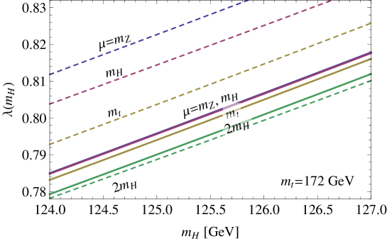
It is common to extrapolate the $\overline{\textrm{MS}}$ top Yukawa coupling $h_{t}(\mu)$ from the matching condition between the running top mass $\overline{m_{t}}(\mu)$ and the top pole mass $m_{t}$:

$$h_{t}(\mu)\frac{v}{\sqrt{2}}=\overline{m_{t}}(\mu)=m_{t}\Bigl{(}1+\delta_{t}(\mu)\Bigr{)}\,\,,\,\,\,\delta_{t}(\mu)=\delta_{t}^{W}(\mu)+\delta_{t}^{QED}(\mu)+\delta_{t}^{QCD}(\mu)\,,$$ (6)

where $\delta_{t}^{W}+\delta_{t}^{QED}$ represent the electroweak contribution, which is known at 1-loop HK , while $\delta_{t}^{QCD}$ is the QCD one. The QCD 1-loop result is known since many years HK ; the QCD 2-loop and 3-loop results as a function of the matching scale $\mu$ are given in Chetyrkin:1999qi (see also GBGS ; BGS ; FJTV ; Melnikov:2000qh ; JK ). The matching is usually done at the top pole mass scale, and the theoretical error associated to the arbitrariness of the matching scale can be estimated as before, namely by comparing the values of $h_{t}(m_{t})$ obtained with different matching scales. This is represented in fig. 2, where the curves are obtained by working at 2-loop and using, from bottom to top, $\mu=m_{Z},m_{t},2m_{t}$. The plot shows that the associated theoretical uncertainty is about $2\%$. The analytical expression for $h_{t}(m_{t})$ is:

$$h_{t}(m_{t})=0.933+0.006\,(m_{t}[{\rm GeV}]-172)\,^{+0.017}_{-0.013}\,\,.$$ (7)

The variations of $h(m_{t})$ due to the experimental range of $\alpha_{s}$ and $m_{H}$ have not been explicitly written in eq.(7) because they are negligible (respectively of order $10\%$ and $1\%$) with respect to the variation of $h(m_{t})$ due to the experimental range of $m_{t}$. The error quoted in eq.(7) then refers only to the theoretical error coming from varying the matching scale $\mu$ from $m_{Z}$, $m_{t}$ (mean value), $2m_{t}$. Notice that our result perfectly agrees with the analogous expression derived in ref. Degrassi:2012ry , where however the error due to the variation of the matching was not estimated.

Figure 2: Values of $h_{t}(m_{t})$ and $\overline{m_{t}}(m_{t})$ as a function of $m_{t}$. The curves are obtained by matching at different scales, which are indicated by the labels. We fixed $m_{H}=126$ GeV for definiteness but the results do not significantly dependent on $m_{H}$, provided it is chosen in its experimental range.

The procedure adopted in previous analyses of the stability of the electroweak vacuum, including the latest ones Bezrukov:2012sa ; Degrassi:2012ry , was to use the experimental value of $m_{t}$, identified with the one measured at the Tevatron by the CDF and D0 collaborations, $m_{t}^{exp}=173.2\pm 0.9$ GeV Lancaster:2011wr , to extrapolate the running Yukawa $h_{t}(m_{t})$ via eq. (7). However, as discussed in ref. Alekhin:2012py , it is not meaningful to use the mass parameter provided by the Tevatron as the pole top mass to be inserted in eq. (7): the running top mass in the $\overline{\rm MS}$ scheme is instead a well defined parameter that can be directly extracted at NNLO from Tevatron measurements of the inclusive top pair production cross-section, giving $\overline{m_{t}}(m_{t})=163.3\pm 2.7$ GeV Alekhin:2012py . So, it is conceptually more robust and practically more convenient to extract the top Yukawa coupling directly from $\overline{m_{t}}(m_{t})$, as will be done in the following. Our results will thus be presented as a function of $\overline{m_{t}}(m_{t})$.

Notice that, according to eq. (7), the value of the top pole mass can be easily recovered via the relation $m_{t}=\overline{m_{t}}(m_{t})+9.6\,^{+2.9}_{-2.3}$ GeV, which however is plagued by a large uncertainty. In ref. Alekhin:2012py it was found that, by doing a scheme transformation to NNLO accuracy from the running to the pole top mass, the range $\overline{m_{t}}(m_{t})=163.3\pm 2.7$ GeV is equivalent to $m_{t}=173.3\pm 2.8$ GeV. Hence, while displaying our results as a function of $\overline{m_{t}}(m_{t})$ as already stated, motivated by the results of ref. Alekhin:2012py , in some plots (as the one in fig. 5) we will link the value of the top pole mass to the running mass via the simple relation $m_{t}=\overline{m_{t}}(m_{t})+10$ GeV.

Before presenting the results of our analysis in the following sections, we recall that, in order to carefully study the shape of the Higgs potential at high energy, one should consider the renormalization improved effective potential. This can be done by introducing an effective coupling, $\lambda_{eff}(\mu)=\lambda(\mu)+\Delta\lambda(\mu)$, so that

$$V_{eff}(\phi_{H})=\frac{\lambda_{eff}(\mu)}{24}\phi_{H}^{4}\,\,\,.$$ (8)

The expression for $\Delta\lambda(\mu)$ is known up to 2-loop FJSE ; 2group (and given, for instance, in Degrassi:2012ry ). Since the scalar contribution is not well defined when $\lambda$ is negative (a logarithm of a negative quantity appears), in the following we consider the renormalization improved potential at the tree level, and identify $\mu$ with $\phi_{H}$. It is well known that this simplification has a negligible impact in the determination of the vacuum stability bound (for a detailed discussion see e.g. ref. Bezrukov:2012sa ) to be discussed in the next section.

III Electroweak Vacuum Stability

The experimental region of the values of the Higgs and top masses is very intriguing from the theoretical point of view, since the Higgs quartic coupling could be rather small, vanish or even turn negative at a scale slightly smaller than the Planck scale. Accordingly, the behavior of the Higgs potential at high energy changes drastically: if $\lambda(\mu)$ is always positive, the electroweak vacuum is a global minimum, possibly accompanied by another local minimum just below the Planck scale, which could have played a role in primordial inflation Masina:2011un ; Masina:2011aa ; Masina:2012yd ; if $\lambda(\mu)$ turns negative below $M_{\rm Pl}$, the electroweak vacuum correspondingly becomes metastable 2group ; 3group .

Figure 3: The SM Higgs potential (left) and the quartic Higgs coupling (right) as functions of the renormalization scale $\mu$, for $m_{H}=126$ GeV and different values of $\overline{m_{t}}(m_{t})$, increasing from top to bottom by the amount indicated by the labels. The dashed curve in the right plot shows the associated value of $\beta_{\lambda}(\mu)$. The other input parameters are fixed at the central values discussed in the previous section.

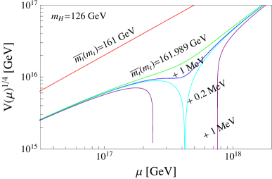
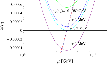
These drastically different possibilities for the behavior of the renormalization improved Higgs potential at high energy are illustrated in the left plot fig. 3, where $m_{H}=126$ GeV and some specific values for $\overline{m_{t}}(m_{t})$ have been selected, increasing from top to bottom. The right plot shows the associated values of $\lambda(\mu)$. Let start considering the value $\overline{m_{t}}(m_{t})=161.989$ GeV. Increasing the latter by just $1$ MeV, the potential develops an inflection point; notice that the associated $\lambda(\mu)$ becomes as small as ${\cal O}(10^{-5})$. Increasing again $\overline{m_{t}}(m_{t})$ by about $200$ keV, the minimum of $\lambda(\mu)$ is equal to zero: a second vacuum degenerate with the electroweak one is obtained. Further increasing $\overline{m_{t}}(m_{t})$ makes $\lambda(\mu)$ turn negative: the electroweak vacuum becomes metastable.

The dashed curve in the right plot in fig. 3 shows the evolution of $\beta_{\lambda}(\mu)=d\lambda(\mu)/dt$ for the same parameter values; there is only a single dashed curve because $\beta_{\lambda}(\mu)$ mildly depends on $\overline{m_{t}}(m_{t})$ if the latter is in the range $161-163$ GeV. Let call $\mu_{\beta}$ the renormalization scale such that $\beta_{\lambda}(\mu_{\beta})=0$. Clearly, only in the case of two degenerate vacua the conditions $\beta_{\lambda}(\mu_{\beta})=0$ and $\lambda(\mu_{\beta})=0$ are simultaneously met. For a shallow false minimum we instead have $\beta_{\lambda}(\mu_{\beta})=0$ and $\lambda(\mu_{\beta})={\cal O}(10^{-5})$, as already mentioned.

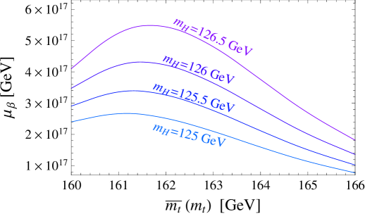
In fig. 4 we show how $\mu_{\beta}$ depends on $\overline{m_{t}}(m_{t})$, for various values of $m_{H}$. It is interesting that $\mu_{\beta}$ is maximized and nearly constant for the values of $\overline{m_{t}}(m_{t})$ for which $\lambda(\mu)$ is very small.

Figure 4: The scale $\mu_{\beta}$ as a function of $\overline{m_{t}}(m_{t})$ and for different values of $m_{H}$, as indicated by the labels.

We now turn to the determination of the points in the plane $[m_{H},\overline{m_{t}}(m_{t})]$ allowing for the existence of a second minimum degenerate with the electroweak one. These points belong to a line separating the stability from the metastability region, see fig. 5: in the lower part of the plot $\lambda(\mu)$ is always positive, while in the upper part it becomes negative before reaching the Planck scale. The configuration of a shallow false minimum belongs to the stability region, but the associated points are so close to the transition line that they could not be distinguished visually.

Figure 5: The solid (black) line marks the points in the plane $[m_{H},\overline{m_{t}}(m_{t})]$ where a second vacuum, degenerate with the electroweak one, is obtained just below the Planck scale. The (red) diagonal arrow shows the effect of varying $\alpha_{3}(m_{Z})=0.1196\pm 0.0017$ PDG ; the (blue) horizontal one shows the effect of varying $\mu_{\lambda}$ (the matching scale of $\lambda$) from $m_{Z}$ up to $2m_{H}$. The shaded (yellow) vertical region is the $2\sigma$ ATLAS :2012gk and CMS :2012gu combined range, $m_{H}=125.65\pm 0.85$ GeV; the shaded (green) horizontal region is the range $\overline{m_{t}}(m_{t})=163.3\pm 2.7$ GeV, equivalent to $m_{t}=173.3\pm 2.8$ GeV Alekhin:2012py .

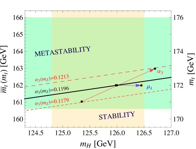
The transition line of fig. 5 was obtained with the input parameter values discussed in the previous section and by matching the running Higgs quartic coupling at $m_{H}$. Clearly, it is also important to estimate the theoretical error associated to experimental ranges of the input parameters and the one associated to the matching procedure. To illustrate this, we consider in particular the point on the transition line associated to the value $m_{H}=126$ GeV; for such point, $\lambda$ and $\beta_{\lambda}$ both vanish at a certain scale $\mu_{\beta}$ (see fig. 4). The arrows show how, if some inputs or the matching scale are changed, the position of this point have to change in order to keep having, at the same scale $\mu_{\beta}$, a vacuum degenerate with the electroweak one. The diagonal arrow is obtained by varying the strong coupling in its allowed range, $\alpha_{3}(m_{Z})=0.1196\pm 0.0017$ PDG ; the short (long) dashed line shows how the solid line would move if $\alpha_{3}(m_{Z})$ were equal to its minimum (maximum) presently allowed value. Notice that the error on $\alpha_{3}(m_{Z})$ induces an uncertainty in both the Higgs and top masses of about $\pm 0.7$ GeV. In ref.Degrassi:2012ry the impact of the variation of $\alpha_{3}(m_{Z})$ on $m_{H}$ was estimated to be $\pm 0.5$ GeV (see their table 1). The two results are in substantial agreement, considering that in our analysis $\alpha_{3}(m_{Z})=0.1196\pm 0.0017$ at $1\sigma$ PDG , while ref.Degrassi:2012ry considers a smaller error, $\alpha_{3}(m_{Z})=0.1184\pm 0.0007$ at $1\sigma$. Since the variation of the other input parameters in eq.(II) induces much smaller effects then the one due to $\alpha_{3}(m_{Z})$, they have not been reported in the fig.5. The horizontal arrow represents instead the theoretical error obtained by varying $\mu_{\lambda}$, the matching scale of the Higgs quartic coupling, from $\mu=m_{Z}$ to $\mu=2m_{H}$; notice that the associated error is very asymmetric (see fig. 1): essentially it can only enhance $m_{H}$, by at most $0.5$ GeV. Clearly, similar considerations apply to each point of the transition line. We note that in ref.Degrassi:2012ry the impact of the variation of the matching scale of $\lambda$ on $m_{H}$ was estimated to be $\pm 0.7$ GeV (see their table 1), hence close to our estimate but with a symmetric error.

Fig. 5 shows that stability can be achieved in the whole experimental range for $m_{H}$ (shaded vertical region), but this is not the case for $\overline{m_{t}}(m_{t})$ (shaded horizontal region). So, it is convenient to write down the condition of electroweak vacuum stability under the form of an upper bound on the running top mass:

$$\overline{m_{t}}(m_{t})[{\rm GeV}]\leq 162.0+0.47\,(m_{H}[{\rm GeV}]-126)+0.7\,\left(\frac{\alpha_{3}(m_{Z})-0.1196}{0.0017}\right)-0.2^{(\mu_{\lambda})}_{th}\,\,\,,$$ (9)

where the last term accounts for the (very asymmetric) theoretical error induced by the matching of $\lambda$. The latter turns out to be smaller than the variation induced by varying $\alpha_{3}(m_{Z})$ in its presently allowed experimental range. We recall that the relation between the running and pole top mass is simply $m_{t}=\overline{m_{t}}(m_{t})+10$ GeV. Fig. 6 summarizes our results for the determination of the transition line between stability and metastability in the $[m_{H},m_{t}]$ plane. The three lines correspond to the central and $\pm 1\sigma$ values of $\alpha_{3}(m_{Z})$ PDG and their thickness represents the theoretical error due to the matching of $\lambda$. The shaded rectangle emphasizes the present allowed region for $m_{t}$ Alekhin:2012py and $m_{H}$ :2012gk ; :2012gu . According to our analysis it is not possible, given the present experimental situation, to understand whether we live in a stable or metastable vacuum configuration.

Figure 6: The transition line between stability and metastability in the plane $[m_{H},m_{t}]$ and for fixed values of $\alpha_{3}(m_{Z})=0.1196\pm 0.0017$ PDG . The thickness of the lines represents the theoretical error due to the variation of $\mu_{\lambda}$ (the matching scale of $\lambda$) from $m_{Z}$ up to $2m_{H}$. The shaded region is obtained by intersecting the $2\sigma$ ATLAS :2012gk and CMS :2012gu combined range ($m_{H}=125.65\pm 0.85$ GeV) with the running top mass range given by ref.Alekhin:2012py , $\overline{m_{t}}(m_{t})=163.3\pm 2.7$ GeV, equivalent to $m_{t}=173.3\pm 2.8$ GeV .

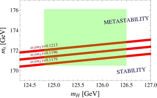
In order to discriminate between the two possibilities, it would be crucial to better determine $\overline{m_{t}}(m_{t})$. As discussed in Alekhin:2012py , after LHC the Higgs mass will presumably be known with an accuracy of ${\cal O}(100)$ MeV futuremh , but the precision on the top mass would improve only by a factor of two. For instance, if the whole range of $\overline{m_{t}}(m_{t})<163$ GeV (or, equivalently $m_{t}<173$ GeV) would be excluded, we would conclude that our vacuum is metastable; otherwise the investigations should continue.

A self-consistent and precise determination of the top quark mass can best be performed at a high-energy electron-positron collider, with a planned accuracy of ${\cal O}(100)$ MeV. Moreover, at an electron-positron collider $\alpha_{3}(m_{Z})$ could be determined with an accuracy close to or better than $\Delta\alpha_{3}(m_{Z})=0.0007$ (this precision is sometimes currently adopted Bezrukov:2012sa ; Degrassi:2012ry but cannot be considered to be conservative according to ref. Alekhin:2012py ). At this stage, if the stability region will still have an overlap with the allowed ranges of the top and Higgs masses, we will be mostly limited by the theoretical uncertainty associated to $\mu_{\lambda}$. Notice also that it is not realistic to hope to distinguish the case of two degenerate minima with the one of a shallow false minimum, since the difference in the top mass is just about $200$ keV (see fig. 3).

We now discuss how to compare eq. (9) and fig. 6 with previous literature results, in particular those of ref. Degrassi:2012ry , since the authors claimed that ”absolute stability of the Higgs potential is excluded at $98\%$ C.L. for $m_{H}<126$ GeV” (see also their fig. 5). In the latter work the stability condition is indeed expressed under the form of a lower bound on the Higgs mass: $m_{H}\geq 129.4+1.4\,(m_{t}-173.1)/0.7-0.5\,(\alpha_{3}(m_{Z})-0.1184)/0.0007\pm 1_{th}$, where all masses are in GeV and the last term represents the overall theoretical error. Combining in quadrature their theoretical uncertainty and their experimental errors on $m_{t}$ and $\alpha_{3}(m_{Z})$, the authors derive $m_{H}>129.4\pm 1.8$ GeV, which motivates the quoted claim of ref. Degrassi:2012ry . In order to carry out the comparison, one must rewrite the inequality of Degrassi:2012ry under a form directly comparable with eq.(9), namely:

$$m_{t}^{[14]}[{\rm GeV}]\leq 171.8+0.5\,(m_{H}[{\rm GeV}]-126)+0.61\,\left(\frac{\alpha_{3}(m_{Z})-0.1196}{0.0017}\right)\pm 0.5_{th}\,.$$ (10)

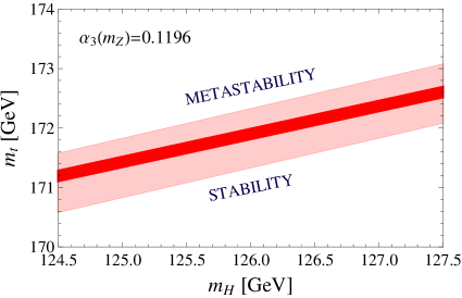
So, our results eq. (9) and the one obtained in ref. Degrassi:2012ry are perfectly compatible, as the central value of eq. (10) essentially overlaps with the lower value of eq. (9). The theoretical error in eq. (9) is however smaller than the theoretical error of ref. Degrassi:2012ry : this is mainly due to the fact that in the present analysis we used directly the running top mass, thus avoiding to introduce the theoretical error due to the matching scale of the top Yukawa coupling (see table 1 of ref. Degrassi:2012ry ). The left plot of fig. 7 shows the comparison between eq. (9) and eq. (10) in the determination of the transition line between stability and metastability in the $[m_{H},m_{t}]$ plane; we choose $\alpha_{3}(m_{Z})=0.1196$ for definiteness, so that the thickness of the lines represents just the theoretical error. According to eq. (9) the thickness of the line is $0.2$ GeV, while according to eq. (10) it is $1$ GeV (as can also be checked by inspecting table 1 of Degrassi:2012ry ).

Figure 7: Left: Theoretical uncertainty in the determination of the transition line between stability and metastability according to our eq. (9) (thinner) and eq. (10) of ref. Degrassi:2012ry (thicker). For definiteness we choose $\alpha_{3}(m_{Z})=0.1196$. Right: transition line between stability and metastability according to eq. (10) of ref. Degrassi:2012ry ; the thickness of the band accounts for both the $1$ GeV theoretical error and the experimental error due to the variation of $\alpha_{3}(m_{Z})$ in the range $0.1184\pm 0.0007$, as done in Degrassi:2012ry . The (brown) shaded disks represent the $1\sigma$ and $2\sigma$ combined ranges for $m_{t}$ and $m_{H}$ used in Degrassi:2012ry (see their fig. 5). The (green) rectangle allows for the comparison with the ranges of $m_{t}$ and $m_{H}$ used here (see fig. 6).

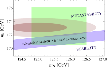
Clearly all these considerations do not justify the different conclusions of the two papers and rather show that the different conclusions have to come from the different ranges used for the three most relevant parameters: $m_{t}$, $m_{H}$ and $\alpha_{3}(m_{Z})$. In ref. Degrassi:2012ry it is assumed that $m_{t}=(173.1\pm 0.7)$ GeV and $m_{H}=(125\pm 1)$ GeV; these errors are further combined in quadrature and the $1\sigma$ and $2\sigma$ (brown) disks in the right plot of fig. 7 are obtained. These disks have to be confronted with our (green) rectangular region, obtained by using $m_{t}=(173.3\pm 2.8)$ GeV, as suggested in ref. Alekhin:2012py , and $m_{H}=(125.65\pm 0.85)$ GeV, as suggested combining the ATLAS :2012gk and CMS :2012gu ranges at $2\sigma$. We have a rectangular region since we think that in this kind of analysis it is not really justified to combine in quadrature the errors on $m_{t}$ and $m_{H}$, thus enhancing the exclusion of the interesting low-$m_{t}$ and high-$m_{H}$ values. A small value of $\alpha_{3}(m_{Z})$ also goes in such direction, since it lowers the transition line towards smaller values of $m_{t}$. In ref. Degrassi:2012ry it is assumed that $\alpha_{3}(m_{Z})=0.1184\pm 0.0007$: the corresponding transition line is displayed in the right plot of fig. 7, using for consistency eq. (10). The line perfectly reproduces the results of fig. 5 of Degrassi:2012ry ; its thickness accounts for both the theoretical error and the experimental error due to the variation of $\alpha_{3}(m_{Z})$, as derived in Degrassi:2012ry . (We cannot display three separate lines as done in fig. 6 since in eq. (10) the theoretical error and the one associated to the variation of $\alpha_{3}(m_{Z})$ are comparable). As the transition line marginally overlaps with the $2\sigma$ disk, the authors of ref. Degrassi:2012ry concluded that stability is disfavored. A very different conclusion would be derived by considering instead the broad overlap with the rectangle. This is the main reason of the different conclusions. A small effect is also played by the different values used for $\alpha_{3}(m_{Z})$. The range of $\alpha_{3}(m_{Z})$ used in ref. Degrassi:2012ry has a very small error and has already been questioned in ref. Alekhin:2012py (see bottom of pag 8). In the present analysis we rather use $\alpha_{3}(m_{Z})=0.1196\pm 0.0017$ PDG , whose central value and experimental error are bigger than those used in ref. Degrassi:2012ry . As an effect, the ensemble of the three (red) lines in fig. 6 forms a band slightly wider and higher than the (blue) band in fig. 7 depicting the results of Degrassi:2012ry .

Summarizing, upon comparison of our results in fig. 6 with the results of ref. Degrassi:2012ry reproduced in the right plot of fig. 7, one can conclude that the difference in the physical interpretation of the results is mainly due to the fact that ref. Degrassi:2012ry adopts a too small experimental error for $m_{t}$, as already pointed out in ref. Alekhin:2012py .

IV Shallow false minimum

It is interesting to study in some detail the boundary conditions which must be satisfied in order to have a very shallow false minimum just below the Planck scale, since it could be relevant for inflation Masina:2011un ; Masina:2011aa ; Masina:2012yd .

To study this particular configuration, we denote with $\mu_{i}$ the renormalization scale where the Higgs potential has an inflection point; we also recall that $\mu_{\beta}$ has been defined to be the scale where $\lambda(\mu_{\beta})=0$ and $\beta_{\lambda}(\mu_{\beta})=0$ are simultaneously fulfilled. Both $\mu_{i}$ and $\mu_{\beta}$ increase with $m_{H}$, as shown in fig. 8, where the shaded region accounts for the experimental range of $\alpha_{3}(m_{Z})$.

Figure 8: Values of $\mu_{i}$ (left) and $\mu_{\beta}$ (right) as a function of $m_{H}$. For the solid lines, the input parameters are fixed at their central values and the matching of $\lambda$ is done at $\mu=m_{H}$. The shaded regions shows the uncertainty induced by the experimental error of $\alpha_{3}(m_{Z})=0.1196\pm 0.0017$: the short and long dashed curves refer to the lower and upper value at $1\sigma$, respectively.

Figure 9: Left: the value of $\lambda(\mu_{\beta})$ as a function of $m_{H}$. Right: the Higgs potential at $\mu_{i}$ and the associated prediction for $r$ as a function of $m_{H}$. The short and long dashed curves refer to the $1\sigma$ lower and upper values of $\alpha_{3}(m_{Z})$, respectively. The shaded (yellow) vertical region marks the preferred range of $m_{H}$ at $2\sigma$ :2012gk ; :2012gu . The upper region in the right plot is excluded because $r\lesssim 0.2$ Komatsu:2010fb .

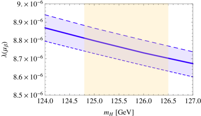
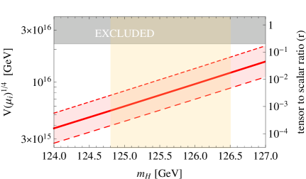
It is interesting that, for the whole experimental range of $m_{H}$, a shallow false minimum is obtained only if the following boundary condition holds:

$$\lambda(\mu_{\beta})\simeq(8.75\pm 0.15)\times 10^{-6}\,\,\,\,.\,\,$$ (11)

One could speculate that such value could be originated by some quantum gravity effect  Holthausen:2011aa ; Shaposhnikov:2009pv . In the left plot of fig. 9 we show that $\lambda(\mu_{\beta})$ has a mild dependence on $m_{H}$; in the right plot we show instead the value of the Higgs potential at the inflection point, which turns out to be of ${\cal O}(10^{16})$ GeV. As before, the shaded regions account for the experimental range of $\alpha_{3}(m_{Z})$.

As pointed out in Masina:2011un , a way of testing the hypothesis that inflation occurred when the Higgs field was trapped into a shallow false vacuum below the Planck scale is to look at the tensor-to-scalar ratio $r$ of cosmological perturbations. The amplitude of density fluctuations in the observed Universe as seen by the CMB and Large-Scale structure data is parametrized by the power spectrum in $k$-space, $P_{s}(k)=\Delta_{R}^{2}\left(k/k_{0}\right)^{n_{S}-1}$, where $\Delta_{R}^{2}$ is the amplitude at some pivot point $k_{0}$, whose best-fit value is $\Delta_{R}^{2}=(2.43\pm 0.11)\times 10^{-9}$ at $k_{0}=0.002\,{\rm Mpc}^{-1}$ Komatsu:2010fb . In models where inflation happened while the Higgs was trapped in the shallow minimum Masina:2011aa ; Masina:2012yd , the Higgs potential at the inflection point and the amount of gravity waves that can be produced - parametrized via the tensor-to-scalar ratio $r$ - are linked via a simple relation:

$$\Delta_{R}^{2}=\frac{2}{3\pi^{2}}\frac{1}{r}\frac{V(\mu_{i})}{M^{4}}\,\,,$$ (12)

where $M$ is the reduced Planck scale. Such prediction for $r$ is reported in the right plot of fig. 9. Notice that, for these models, only if $m_{H}$ is in its upper allowed range and $\alpha_{3}(m_{Z})$ is quite low, there are chances for the Planck satellite mission Planck:2006aa to measure $r$. However, the forthcoming experiment EPIC Bock:2009xw should be able to test $r$ down to $10^{-2}$, while COrE Bouchet:2011ck down to about $10^{-3}$.

V Constraints on the Seesaw Mechanism

We now consider the effect of including neutrino masses via a type I seesaw. This issue has been already considered in a series of papers Casas:1999cd ; Gogoladze:2008ak ; EliasMiro:2011aa ; Rodejohann:2012px ; Chakrabortty:2012np .

Although the precise amount of the effect is quite model dependent, here we obtain a conservative estimate of the effect by considering only one right handed neutrino with mass $M_{\nu}$, associated to a light Majorana neutrino with mass $m_{\nu}=0.06$ eV, the scale of the atmospheric oscillations. This is supported by the following argument.

It is well known that the $\beta$-function of the Higgs quartic coupling is affected only if $h_{\nu}(\mu)$, the Yukawa coupling of the Dirac mass term (defined only for $\mu\geq M_{\nu}$), is large enough. As the top Yukawa coupling, also the neutrino Yukawa coupling induces a suppression of the Higgs quartic coupling at high energy. By increasing $M_{\nu}$ and $m_{\nu}$, the neutrino Yukawa coupling at the threshold scale $M_{\nu}$ also increases:

$$h_{\nu}(M_{\nu})=2\sqrt{\frac{m_{\nu}(M_{\nu})\,M_{\nu}}{v^{2}}}\,\,.$$ (13)

This justifies that the fact that we equate $m_{\nu}$ to the the atmospheric mass scale, about $0.06$ eV, which is the lowest possible value for the heaviest among the three light neutrinos. In addition, two other Majorana neutrinos with masses lighter than $m_{\nu}$ can be accommodated via the seesaw but, if their right-handed neutrinos are lighter than $M_{\nu}$, the associated Dirac Yukawa couplings are naturally expected to be smaller, and their effect on $\lambda(\mu)$ negligible.

In Appendix B we provide the additional terms (with respect to the pure SM) for the relevant $\beta$-functions, above and below the scale $M_{\nu}$.

Figure 10: Upper bound on $M_{\nu}$ as a function of the running top mass, following from the requirement that the electroweak vacuum is not destabilized because of the inclusion of the seesaw, for $m_{H}=126$ GeV. The shaded region is obtained by varying $\alpha_{3}(m_{Z})$ in its $1\sigma$ range.

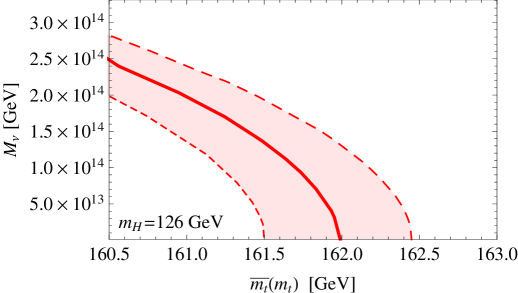
Since the effect of $h_{\nu}$ is a suppression of $\lambda$, a SM configuration with a stable electroweak vacuum could be rendered metastable because of the addition of the seesaw interactions. For a fixed value of $m_{H}$, and in the range of the top mass values allowing the electroweak vacuum to be the global one, one can find the upper bound on $M_{\nu}$ following from the requirement that the electroweak vacuum remains the global one even after the inclusion of the seesaw interactions. Clearly such upper limit cannot be derived in the range of the top mass values for which the electroweak vacuum is already metastable. As shown in fig. 10 for $m_{H}=126$ GeV (but similar upper bounds are obtained in the whole experimental range of $m_{H}$), such upper bound strongly depends on the top mass and is affected by an uncertainty which is mainly due to $\alpha_{3}(m_{Z})$ (shaded region). The smaller the top mass is, the more the configuration of the Higgs potential is stable and the less stringent is the $M_{\nu}$ upper bound ensuring that the electroweak vacuum remains the global one and does not become metastable, $M_{\nu}\lesssim 3\times 10^{14}$ GeV. But increasing the top mass, the electroweak vacuum becomes less stable and the upper bound on $M_{\nu}$ becomes accordingly more and more stringent. Increasing further the top mass the electroweak vacuum becomes metastable even without seesaw interactions, so that no meaningful bound can be derived.

The upper bound on $M_{\nu}$ following from the requirement of electroweak vacuum stability has to be taken cum grano salis, in the sense that it is not a physically robust bound, but just a bound that should be respected in the case one has a model in which the Higgs potential has to remain stable for reason.

Let consider in particular the upper bound on $M_{\nu}$ needed to avoid destabilization of an inflection point configuration, as the one depicted via the dashed line in fig. 11. Notice that an inflection point becomes a not so shallow local second minimum if $M_{\nu}\sim 10^{11}$ GeV and that electroweak vacuum destabilization is avoided only if the condition $M_{\nu}\lesssim 2\times 10^{11}$ GeV is satisfied. The latter bound might be relevant for models of inflation based on the SM shallow false minimum Masina:2011un ; Masina:2011aa ; Masina:2012yd ; note however that it is well compatible with the thermal leptogenesis mechanism to explain matter-antimatter asymmetry, for which the lower bound on the lightest Majorana neutrino is about $5\times 10^{8}$ GeV Davidson:2002qv .

Figure 11: The dashed curve represents the Higgs potential as function of the renormalization scale, for $m_{H}=126$ GeV, $\alpha_{3}(m_{Z})=0.1196$ and $m_{t}=171.56$ GeV (the value of the top mass leading to an inflection point configuration in the SM case once fixed the former two parameters). The solid lower curves display the effect of adding the seesaw, with three increasing values of $M_{\nu}$ from top to bottom.

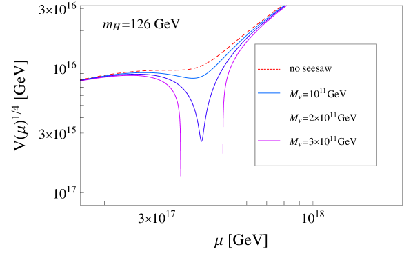
Clearly, the neutrino Yukawa coupling $y_{\nu}$ is not the only additional term beyond the SM capable of modifying the running of $\lambda$ at high energy. Always in the context of type I seesaw, in the case that the vacuum expectation value of a singlet scalar field $S$ (violating the lepton number by two units) is actually at the origin of the right-handed Majorana neutrino mass, the $S$ couplings induce an enhancement of $\lambda$, thus helping the stability of the electroweak vacuum EliasMiro:2012ay . Such effect is indeed generically expected when adding to the SM a singlet field $S$ Lebedev:2012zw ; EliasMiro:2012ay .

VI Conclusions

The recent discovery of a particle consistent with the SM Higgs boson :2012gk ; :2012gu provides a strong motivation to pursue Holthausen:2011aa ; Masina:2011aa ; EliasMiro:2011aa ; Xing:2011aa ; Masina:2011un ; Bezrukov:2012sa ; Degrassi:2012ry ; Alekhin:2012py the old project 1group ; 2group ; 3group of investigating the behavior of the SM Higgs potential at very high energies. In particular, one would understand whether the SM electroweak vacuum is a global minimum up to the Planck scale, namely whether we live in a stable vacuum assuming a desert (or assuming that new interactions do not modify the running of $\lambda$ with respect to the SM case). In particular, a stable configuration which deserves a special interest is a shallow false minimum below the Planck scale: the Higgs field could have been primordially trapped there, leading to a stage of inflation Masina:2011aa ; Masina:2011un ; Masina:2012yd . Stability below the Planck scale is required also in Higgs inflation models with non minimal gravitational couplings  Bezrukov:2007ep ; Bezrukov:2012sa .

In our analysis, we adopted the recently derived tools for a NNLO renormalization procedure Mihaila:2012fm ; Chetyrkin:2012rz ; Bezrukov:2012sa ; Degrassi:2012ry . At difference of previous analyses, we considered as free parameter the running top mass rather than the (Tevatron) top pole mass, as suggested in ref. Alekhin:2012py .

Given the present range of the running top mass and of the Higgs mass, we found that electroweak vacuum stability is at present allowed, as shown in figs. 5 and 6. To further test stability, a more precise measurement of the top mass would be crucial. As apparent from the stability condition of eq. (9), in case that LHC will not exclude values of the running top mass below $163$ GeV (or equivalently values of the pole top mass below $173$ GeV), an electron-positron collider would probably be needed to discriminate between stability and metastability.

We also determined the high scale boundary conditions allowing for a shallow false minimum slightly below the Planck scale, $\lambda(\mu_{\beta})\sim 10^{-5}$ ($\mu_{\beta}$ is the renormalization scale were the $\beta$-function of the Higgs quartic coupling vanishes), and discussed the prospects for the cosmological tests of such configuration. Finally, a conservative upper bound on type I seesaw right-handed neutrino masses, following from the requirement of electroweak vacuum stability, was derived, analyzing in particular its dependence on the top mass.

The present analysis does not consider the effect of the gravitational couplings because it is far from clear how the quantum effects of the latter would impact the study at very high energies. Other sources of uncertainty could also come from the treatment of the effective potential itself, such as the fine-tuning required for both the cosmological constant and the Higgs mass.

Appendix A Formulæ  for the RG running at NNLO

A.1 The $\beta$-functions

Here we provide the expressions for the $\beta$-functions up to 3-loops, see eq. (2).

At 1-loop they are given by:

$$\beta_{\lambda}^{(1)} = \frac{27}{4}g(t)^{4}+\frac{9}{2}g^{\prime}(t)^{2}g(t)^{2}-9\lambda(t)g(t)^{2}+\frac{9}{4}g^{\prime}(t)^{4}-36h_{t}(t)^{4}+4\lambda(t)^{2}-3g^{\prime}(t)^{2}\lambda(t)$$

$$+12h_{t}(t)^{2}\lambda(t)\ ,$$

$$\beta^{(1)}_{h_{t}} = \frac{9}{2}h_{t}(t)^{3}-\frac{9}{4}g(t)^{2}h_{t}(t)-8g_{3}(t)^{2}h_{t}(t)-\frac{17}{12}g^{\prime}(t)^{2}h_{t}(t)\ ,$$

$$\beta_{g}^{(1)} = -\frac{19}{6}g(t)^{3}\ ,$$

$$\beta_{g^{\prime}}^{(1)} = \frac{41}{6}g^{\prime}(t)^{3}\ ,$$

$$\beta_{g_{3}}^{(1)} = -7g_{3}(t)^{3}\ .$$

At 2-loop they are:

$$\beta_{\lambda}^{(2)} = 80g_{3}(t)^{2}h_{t}(t)^{2}\lambda(t)-192g_{3}(t)^{2}h_{t}(t)^{4}+\frac{915}{8}g(t)^{6}-\frac{289}{8}g^{\prime}(t)^{2}g(t)^{4}-\frac{27}{2}h_{t}(t)^{2}g(t)^{4}$$

$$-\frac{73}{8}\lambda(t)g(t)^{4}-\frac{559}{8}g^{\prime}(t)^{4}g(t)^{2}+63g^{\prime}(t)^{2}h_{t}(t)^{2}g(t)^{2}+\frac{39}{4}g^{\prime}(t)^{2}\lambda(t)g(t)^{2}-3h_{t}(t)^{4}\lambda(t)$$

$$+\frac{45}{2}h_{t}(t)^{2}\lambda(t)g(t)^{2}-\frac{379}{8}g^{\prime}(t)^{6}+180h_{t}(t)^{6}-16g^{\prime}(t)^{2}h_{t}(t)^{4}-\frac{26}{3}\lambda(t)^{3}-\frac{57}{2}g^{\prime}(t)^{4}h_{t}(t)^{2}$$

$$-24h_{t}(t)^{2}\lambda(t)^{2}+6\left(3g(t)^{2}+g^{\prime}(t)^{2}\right)\lambda(t)^{2}+\frac{629}{24}g^{\prime}(t)^{4}\lambda(t)+\frac{85}{6}g^{\prime}(t)^{2}h_{t}(t)^{2}\lambda(t)\ ,$$

$$\beta_{h_{t}}^{(2)} = h_{t}(t)\left[-108g_{3}(t)^{4}+9g(t)^{2}g_{3}(t)^{2}+\frac{19}{9}g^{\prime}(t)^{2}g_{3}(t)^{2}+36h_{t}(t)^{2}g_{3}(t)^{2}-\frac{3}{4}g^{\prime}(t)^{2}g(t)^{2}\right.$$

$$\left.-\frac{23}{4}g(t)^{4}+\frac{1187}{216}g^{\prime}(t)^{4}-12h_{t}(t)^{4}+\frac{\lambda(t)^{2}}{6}+h_{t}(t)^{2}\left(\frac{225}{16}g(t)^{2}+\frac{131}{16}g^{\prime}(t)^{2}-2\lambda(t)\right)\right]\ ,$$

$$\beta_{g}^{(2)} = 12g_{3}(t)^{2}g(t)^{3}+\left(\frac{35}{6}g(t)^{2}+\frac{3}{2}g^{\prime}(t)^{2}-\frac{3}{2}h_{t}(t)^{2}\right)g(t)^{3}\ ,$$

$$\beta_{g^{\prime}}^{(2)} = \frac{44}{3}g_{3}(t)^{2}g^{\prime}(t)^{3}+\left(\frac{9}{2}g(t)^{2}+\frac{199}{18}g^{\prime}(t)^{2}-\frac{17}{6}h_{t}(t)^{2}\right)g^{\prime}(t)^{3}\ ,$$

$$\beta_{g_{3}}^{(2)} = g_{3}(t)^{3}\left(\frac{9}{2}g(t)^{2}-26g_{3}(t)^{2}+\frac{11}{6}g^{\prime}(t)^{2}-2h_{t}(t)^{2}\right)\ .$$

The leading terms in the 3-loop $\beta$-functions of $\lambda$ and $h_{t}$ are Chetyrkin:2012rz :

$$\beta_{\lambda}^{(3)} = 12\left[(-\frac{266}{3}+32\zeta_{3})g_{3}(t)^{4}h_{t}(t)^{4}+(-38+240\zeta_{3})g_{3}(t)^{2}h_{t}(t)^{6}-(\frac{1599}{8}+36\zeta_{3})h_{t}(t)^{8}\right.$$

$$+\frac{1}{6}(\frac{1244}{3}-48\zeta_{3})g_{3}(t)^{4}h_{t}(t)^{2}\lambda(t)+\frac{1}{6}(895-1296\zeta_{3})g_{3}(t)^{2}h_{t}(t)^{4}\lambda(t)+$$

$$\frac{1}{6}(\frac{117}{8}-198\zeta_{3})h_{t}(t)^{6}\lambda(t)+\frac{1}{36}(-1224+1152\zeta_{3})g_{3}(t)^{2}h_{t}(t)^{2}\lambda(t)^{2}+$$

$$\frac{1}{36}(\frac{1719}{2}+756\zeta_{3})h_{t}(t)^{4}\lambda(t)^{2}+\left.\frac{97}{24}h_{t}(t)^{2}\lambda(t)^{3}+\frac{1}{1296}(3588+2016\zeta_{3})\lambda(t)^{4}\right]\,,$$

$$\beta_{h_{t}}^{(3)} = 2\left[(-\frac{2083}{3}+320\zeta_{3})g_{3}(t)^{6}+(\frac{3827}{12}-114\zeta_{3})g_{3}(t)^{4}h_{t}(t)^{2}-\frac{157}{2}g_{3}(t)^{2}h_{t}(t)^{4}\right.$$

$$+(\frac{339}{16}+\frac{27}{4}\zeta_{3})h(t)^{6}+\frac{4}{3}g_{3}(t)^{2}h_{t}(t)^{2}\lambda(t)+\frac{33}{2}h_{t}(t)^{4}\lambda(t)+\left.\frac{5}{96}h_{t}(t)^{2}\lambda(t)^{2}-\frac{1}{12}\lambda(t)^{3}\right]\,,$$

where $\zeta_{3}=1.20206...$ is the Riemann zeta function.

The complete 3-loop $\beta$-functions for the gauge couplings are Mihaila:2012fm :

$$\beta_{g}^{(3)} = \frac{324953}{1728}g(t)^{7}+39g(t)^{5}g_{3}(t)^{2}+81g(t)^{3}g_{3}(t)^{4}+\frac{291}{32}g(t)^{5}g^{\prime}(t)^{2}-\frac{1}{3}g(t)^{3}g_{3}(t)^{2}g^{\prime}(t)^{2}$$

$$-\frac{5597}{576}g(t)^{3}g^{\prime}(t)^{4}-\frac{729}{32}g(t)^{5}h_{t}(t)^{2}-7g(t)^{3}g_{3}(t)^{2}h_{t}(t)^{2}-\frac{593}{96}g(t)^{3}g^{\prime}(t)^{2}h_{t}(t)^{2}$$

$$+\frac{147}{16}g(t)^{3}h_{t}(t)^{4}\,,$$

$$\beta_{g^{\prime}}^{(3)} = \frac{1315}{64}g(t)^{4}g^{\prime}(t)^{3}-g(t)^{2}g_{3}(t)^{2}g^{\prime}(t)^{3}+99g_{3}(t)^{4}g^{\prime}(t0^{3}+\frac{205}{96}g(t)^{2}g^{\prime}(t)^{5}-\frac{137}{27}g_{3}(t)^{2}g^{\prime}(t)^{5}$$

$$-\frac{388613}{5184}g^{\prime}(t)^{7}-\frac{785}{32}g(t)^{2}g^{\prime}(t)^{3}h_{t}(t)^{2}-\frac{29}{3}g_{3}(t)^{2}g^{\prime}(t)^{3}h_{t}(t)^{2}-\frac{2827}{288}g^{\prime}(t)^{5}h_{t}(t)^{2}$$

$$+\frac{315}{16}g^{\prime}(t)^{3}h_{t}(t)^{4}\,,$$

$$\beta_{g_{3}}^{(3)} = \frac{109}{8}g(t)^{4}g_{3}(t)^{3}+21g(t)^{2}g_{3}(t)^{5}+\frac{65}{2}g_{3}(t)^{7}-\frac{1}{8}g(t)^{2}g_{3}(t)^{3}g^{\prime}(t)^{2}+\frac{77}{9}g_{3}(t)^{5}g^{\prime}(t)^{2}\,$$

$$-\frac{2615}{216}g_{3}(t)^{3}g^{\prime}(t)^{4}-\frac{93}{8}g(t)^{2}g_{3}(t)^{3}h_{t}(t)^{2}-40g_{3}(t)^{5}h_{t}(t)^{2}+\frac{101}{24}g_{3}(t)^{3}g^{\prime}(t)^{2}h_{t}(t)^{2}\,$$

$$+15g_{3}(t)^{3}h_{t}(t)^{4}\,.$$

A.2 Higgs quartic coupling matching

According to Sirlin and Zucchini SZ , the 1-loop matching is given by

$$\delta^{(1)}_{H}(\mu)=\frac{G_{\mu}m_{Z}^{2}}{8\sqrt{2}\pi^{2}}\left(\xi f_{1}(\mu)+f_{0}(\mu)+\frac{f_{-1}(\mu)}{\xi}\right)\,,$$

where $\xi=\frac{m_{H}^{2}}{m_{Z}^{2}}$ and, introducing $c=\frac{m_{W}}{m_{Z}}$,

$$f_{1}(\mu) = \frac{3}{2}\log(\xi)-\log\left(c^{2}\right)+6\log\left(\frac{\mu^{2}}{m_{H}^{2}}\right)-\frac{1}{2}Z\left[\frac{1}{\xi}\right]-Z\left[\frac{c^{2}}{\xi}\right]+\frac{9}{2}\left(\frac{25}{9}-\frac{\pi}{\sqrt{3}}\right)\,,$$

$$f_{0}(\mu) = \frac{3c^{2}}{s^{2}}\log\left(c^{2}\right)+12\log c^{2}\left(c^{2}\right)+\frac{3\xi c^{2}}{\xi-c^{2}}\log\left(\frac{\xi}{c^{2}}\right)+4c^{2}\,Z\left[\frac{c^{2}}{\xi}\right]-\frac{15}{2}\left(2c^{2}+1\right)$$

$$-6\left(2c^{2}-\frac{2m_{t}^{2}}{m_{Z}^{2}}+1\right)\log\left(\frac{\mu^{2}}{m_{Z}^{2}}\right)-\frac{3m_{t}^{2}}{m_{Z}^{2}}\left(4\log\left(\frac{m_{t}^{2}}{m_{Z}^{2}}\right)+2\,Z\left[\frac{m_{t}^{2}}{m_{Z}^{2}\xi}\right]-5\right)$$

$$+2\,Z\left[\frac{1}{\xi}\right]\,,$$

$$f_{-1}(\mu) = 8\left(2c^{4}+1\right)-12c^{4}\log\left(c^{2}\right)-12c^{4}\,Z\left[\frac{c^{2}}{\xi}\right]+6\left(2c^{4}-\frac{4m_{t}^{4}}{m_{Z}^{4}}+1\right)\log\left(\frac{\mu^{2}}{m_{Z}^{2}}\right)$$

$$-6\,Z\left[\frac{1}{\xi}\right]+\frac{24m_{t}^{4}}{m_{Z}^{4}}\left(\log\left(\frac{m_{t}^{2}}{m_{Z}^{2}}\right)+Z\,\left[\frac{m_{t}^{2}}{m_{Z}^{2}\xi}\right]-2\right)\,,$$

$$Z[z] = \left\{\begin{array}[]{lll}2A(z)\,{\rm arctan}\left(\frac{1}{A(z)}\right)&\textrm{if}&z>\frac{1}{4}\\ A(z)\log\left(\frac{A(z)+1}{1-A(z)}\right)&\textrm{if}&z<\frac{1}{4}\end{array}\right.\,,$$

$$A(z) = \sqrt{|1-4z|}\,.$$

We compute the QCD and the Yukawa contribution to $\lambda^{(2)}(\mu)$ following the expressions of Degrassi:2012ry (multiplied them by a factor of $6$ to compensate for the different definition of the quartic coupling).

Appendix B Seesaw contribution to the $\beta$-functions

Below the right handed neutrino mass scale, the running of the effective light Majorana neutrino mass is given by Babu:1993qv

$$\frac{dm_{\nu}(t)}{dt}=\kappa\left(-3g_{2}(t)^{2}+6h_{t}(t)^{2}+\frac{\lambda(t)}{6}\right)m_{\nu}(t)\,\,.$$

For $\mu>M_{\nu}$, we have Pirogov:1998tj

$$\frac{dh_{\nu}(t)}{dt}=\kappa\,h_{\nu}(t)\left(\frac{5}{4}h_{\nu}(t)^{2}+\frac{3}{2}h_{t}(t)^{2}-\frac{3}{4}g^{\prime}(t)^{2}-\frac{9}{4}g(t)^{2}\right)\,\,,$$

together with

$$\delta\beta^{(1)}_{\lambda}=-3h_{\nu}(t)^{4}+2\lambda(t)h_{\nu}(t)^{2}\,\,\,,\,\,\,\delta\beta^{(1)}_{h_{t}}=\frac{1}{2}h_{\nu}(t)^{2}\,\,.$$

References

- (1) G. Aad et al. [ATLAS Collaboration], Phys. Lett. B [arXiv:1207.7214 [hep-ex]].
- (2) S. Chatrchyan et al. [CMS Collaboration], Phys. Lett. B [arXiv:1207.7235 [hep-ex]].
- (3) P. Q. Hung, Phys. Rev. Lett. 42 (1979) 873. N. Cabibbo, L. Maiani, G. Parisi and R. Petronzio, Nucl. Phys. B 158 (1979) 295. M. Lindner, Z. Phys. C 31 (1986) 295. M. Lindner, M. Sher and H. W. Zaglauer, Phys. Lett. B 228 (1989) 139. M. Sher, Phys. Rept. 179 (1989) 273. M. Sher, Phys. Lett. B 317, 159 (1993) [Addendum-ibid. B 331, 448 (1994)] [arXiv:hep-ph/9307342]. G. Altarelli and G. Isidori, Phys. Lett. B 337, 141 (1994). C. D. Froggatt and H. B. Nielsen, Phys. Lett. B 368 (1996) 96 [hep-ph/9511371]. B. Schrempp and M. Wimmer, Prog. Part. Nucl. Phys. 37 (1996) 1 [hep-ph/9606386].
- (4) J. A. Casas, J. R. Espinosa and M. Quiros, Phys. Lett. B 342, 171 (1995) [arXiv:hep-ph/9409458]. J. R. Espinosa and M. Quiros, Phys. Lett. B 353, 257 (1995) [arXiv:hep-ph/9504241]. J. A. Casas, J. R. Espinosa and M. Quiros, Phys. Lett. B 382 (1996) 374 [hep-ph/9603227].
- (5) G. Isidori, G. Ridolfi and A. Strumia, Nucl. Phys. B 609 (2001) 387 [hep-ph/0104016]. J. R. Espinosa, G. F. Giudice and A. Riotto, JCAP 0805 (2008) 002 [arXiv:0710.2484 [hep-ph]]. G. Isidori, V. S. Rychkov, A. Strumia and N. Tetradis, Phys. Rev. D 77 (2008) 025034 [arXiv:0712.0242 [hep-ph]]. N. Arkani-Hamed, S. Dubovsky, L. Senatore and G. Villadoro, JHEP 0803 (2008) 075 [arXiv:0801.2399 [hep-ph]]. J. Ellis, J. R. Espinosa, G. F. Giudice, A. Hoecker and A. Riotto, Phys. Lett. B 679 (2009) 369 [arXiv:0906.0954 [hep-ph]].
- (6) M. Holthausen, K. S. Lim and M. Lindner, JHEP 1202 (2012) 037 [arXiv:1112.2415 [hep-ph]].
- (7) I. Masina and A. Notari, Phys. Rev. D 85 (2012) 123506 [arXiv:1112.2659 [hep-ph]].
- (8) J. Elias-Miro, J. R. Espinosa, G. F. Giudice, G. Isidori, A. Riotto and A. Strumia, Phys. Lett. B 709 (2012) 222 [arXiv:1112.3022 [hep-ph]].
- (9) Z. -z. Xing, H. Zhang and S. Zhou, Phys. Rev. D 86 (2012) 013013 [arXiv:1112.3112 [hep-ph]].
- (10) ATLAS Collaboration, Phys. Lett. B 710, 49 (2012); Phys. Rev. Lett. 108, 111803 (2012); arXiv:1202.1415 [hep-ex]. CMS Collaboration, arXiv:1202.1488 [hep-ex].
- (11) L. N. Mihaila, J. Salomon and M. Steinhauser, Phys. Rev. Lett. 108 (2012) 151602 [arXiv:1201.5868 [hep-ph]].
- (12) K. G. Chetyrkin and M. F. Zoller, JHEP 1206 (2012) 033 [arXiv:1205.2892 [hep-ph]].
- (13) F. Bezrukov, M. Y. Kalmykov, B. A. Kniehl and M. Shaposhnikov, arXiv:1205.2893 [hep-ph].
- (14) G. Degrassi, S. Di Vita, J. Elias-Miro, J. R. Espinosa, G. F. Giudice, G. Isidori and A. Strumia, JHEP 1208 (2012) 098 [arXiv:1205.6497 [hep-ph]].
- (15) S. Alekhin, A. Djouadi and S. Moch, arXiv:1207.0980 [hep-ph].
- (16) [Tevatron Electroweak Working Group and CDF and D0 Collaborations], arXiv:1107.5255 [hep-ex].
- (17) I. Masina and A. Notari, Phys. Rev. Lett. 108 (2012) 191302 [arXiv:1112.5430 [hep-ph]].
- (18) I. Masina and A. Notari, arXiv:1204.4155 [hep-ph].
- (19) J. Beringer et al. (Particle Data Group), “Review of particle physics”, Phys. Rev. D86, 010001 (2012)
- (20) C. Ford, D. R. T. Jones, P. W. Stephenson and M. B. Einhorn, Nucl. Phys. B 395, 17 (1993) [arXiv:hep-lat/9210033]; C. Ford, I. Jack and D. R. T. Jones, Nucl. Phys. B 387 (1992) 373 [Erratum-ibid. B 504 (1997) 551] [arXiv:hep-ph/0111190].
- (21) D. J. Gross and F. Wilczek, Phys. Rev. Lett. 30 (1973) 1343. D. J. Gross and F. Wilczek, Phys. Rev. D 8 (1973) 3633. H. D. Politzer, Phys. Rev. Lett. 30 (1973) 1346. D. R. T. Jones, Nucl. Phys. B 75 (1974) 531. W. E. Caswell, Phys. Rev. Lett. 33 (1974) 244.
- (22) O. V. Tarasov and A. A. Vladimirov, Sov. J. Nucl. Phys. 25 (1977) 585 [Yad. Fiz. 25 (1977) 1104]. O. V. Tarasov, A. A. Vladimirov and A. Y. Zharkov, Phys. Lett. B 93, 429 (1980); D. R. T. Jones, M. Fischler and J. Oliensis, Phys. Lett. B 119 (1982) 385. M. E. Machacek and M. T. Vaughn, Nucl. Phys. B 222 (1983) 83. M. E. Machacek and M. T. Vaughn, Nucl. Phys. B 236 (1984) 221. M. E. Machacek and M. T. Vaughn, Nucl. Phys. B 249 (1985) 70.
- (23) S. A. Larin and J. A. M. Vermaseren, Phys. Lett. B 303, 334 (1993) [arXiv:hep-ph/9302208].
- (24) T. van Ritbergen, J. A. M. Vermaseren and S. A. Larin, Phys. Lett. B 400, 379 (1997) [arXiv:hep-ph/9701390].
- (25) M. -x. Luo and Y. Xiao, Phys. Rev. Lett. 90 (2003) 011601 [hep-ph/0207271].
- (26) M. Czakon, Nucl. Phys. B 710, 485 (2005) [arXiv:hep-ph/0411261].
- (27) A. Sirlin and R. Zucchini, Nucl. Phys. B 266, 389 (1986).
- (28) R. Hempfling and B. A. Kniehl, Phys. Rev. D 51, 1386 (1995) [arXiv:hep-ph/9408313].
- (29) K. G. Chetyrkin and M. Steinhauser, Nucl. Phys. B 573 (2000) 617 [hep-ph/9911434].
- (30) N. Gray, D. J. Broadhurst, W. Grafe and K. Schilcher, Z. Phys. C 48, 673 (1990).
- (31) D. J. Broadhurst, N. Gray and K. Schilcher, Z. Phys. C 52, 111 (1991).
- (32) J. Fleischer, F. Jegerlehner, O. V. Tarasov and O. L. Veretin, Nucl. Phys. B 539, 671 (1999) [Erratum-ibid. B 571, 511 (2000)] [arXiv:hep-ph/9803493].
- (33) K. Melnikov and T. v. Ritbergen, Phys. Lett. B 482 (2000) 99 [hep-ph/9912391].
- (34) F. Jegerlehner and M. Y. Kalmykov, Nucl. Phys. B 676, 365 (2004) [arXiv:hep-ph/0308216].
- (35) G. Aad et al. [ATLAS Collaboration], arXiv:0901.0512 [hep-ex]. G. L. Bayatian et al. [CMS Collaboration], J. Phys. G G 34 (2007) 995.
- (36) M. Shaposhnikov and C. Wetterich, Phys. Lett. B 683 (2010) 196 [arXiv:0912.0208 [hep-th]].
- (37) E. Komatsu et al. [WMAP Collaboration], Astrophys. J. Suppl. 192 (2011) 18 [arXiv:1001.4538 [astro-ph.CO]].
- (38) [Planck Collaboration], astro-ph/0604069. See also: C. Burigana, C. Destri, H. J. de Vega, A. Gruppuso, N. Mandolesi, P. Natoli and N. G. Sanchez, Astrophys. J. 724 (2010) 588 [arXiv:1003.6108 [astro-ph.CO]].
- (39) J. Bock et al. [EPIC Collaboration], arXiv:0906.1188 [astro-ph.CO].
- (40) F. R. Bouchet et al. [COrE Collaboration], arXiv:1102.2181 [astro-ph.CO].
- (41) J. A. Casas, V. Di Clemente, A. Ibarra and M. Quiros, Phys. Rev. D 62 (2000) 053005 [hep-ph/9904295].
- (42) I. Gogoladze, N. Okada and Q. Shafi, Phys. Lett. B 668 (2008) 121 [arXiv:0805.2129 [hep-ph]].
- (43) W. Rodejohann and H. Zhang, JHEP 1206 (2012) 022 [arXiv:1203.3825 [hep-ph]].
- (44) J. Chakrabortty, M. Das and S. Mohanty, arXiv:1207.2027 [hep-ph].
- (45) S. Davidson and A. Ibarra, Phys. Lett. B 535 (2002) 25 [hep-ph/0202239].
- (46) J. Elias-Miro, J. R. Espinosa, G. F. Giudice, H. M. Lee and A. Strumia, JHEP 1206 (2012) 031 [arXiv:1203.0237 [hep-ph]]. See also: L. Basso, S. Moretti and G. M. Pruna, Phys. Rev. D 82 (2010) 055018 [arXiv:1004.3039 [hep-ph]].
- (47) O. Lebedev, Eur. Phys. J. C 72 (2012) 2058 [arXiv:1203.0156 [hep-ph]].
- (48) F. L. Bezrukov and M. Shaposhnikov, Phys. Lett. B 659 (2008) 703 [arXiv:0710.3755 [hep-th]]. F. Bezrukov and M. Shaposhnikov, JHEP 0907 (2009) 089 [arXiv:0904.1537 [hep-ph]]. F. Bezrukov, D. Gorbunov and M. Shaposhnikov, JCAP 1110 (2011) 001 [arXiv:1106.5019 [hep-ph]]. For a classification of models with non minimal couplings see: K. Kamada, T. Kobayashi, T. Takahashi, M. Yamaguchi and J. ’i. Yokoyama, Phys. Rev. D 86 (2012) 023504 [arXiv:1203.4059 [hep-ph]].
- (49) K. S. Babu, C. N. Leung and J. T. Pantaleone, Phys. Lett. B 319 (1993) 191 [hep-ph/9309223].
- (50) Y. F. Pirogov and O. V. Zenin, Eur. Phys. J. C 10 (1999) 629 [hep-ph/9808396].