Statistical properties of power-law random banded unitary matrices in the delocalization-localization transition regime

Abstract

Power-law random banded unitary matrices (PRBUM), whose matrix elements decay in a power-law fashion, were recently proposed to model the critical statistics of the Floquet eigenstates of periodically driven quantum systems. In this work, we numerically study in detail the statistical properties of PRBUM ensembles in the delocalization-localization transition regime. In particular, implications of the delocalization-localization transition for the fractal dimension of the eigenvectors, for the distribution function of the eigenvector components, and for the nearest neighbor spacing statistics of the eigenphases are examined. On the one hand, our results further indicate that a PRBUM ensemble can serve as a unitary analog of the power-law random Hermitian matrix model for Anderson transition. On the other hand, some statistical features unseen before are found from PRBUM. For example, the dependence of the fractal dimension of the eigenvectors of PRBUM upon one ensemble parameter displays features that are quite different from that for the power-law random Hermitian matrix model. Furthermore, in the time-reversal symmetric case the nearest neighbor spacing distribution of PRBUM eigenphases is found to obey a semi-Poisson distribution for a broad range, but display an anomalous level repulsion in the absence of time-reversal symmetry.

1 Introduction

As a statistical description with few parameters, random matrix theory (RMT) mehta has found important applications in a wide variety of topics, such as complex heavy nuclei porter , disordered electronic systems disorder , large complex atoms camrada , stock market data analysis market , atmospheric data analysis santh , analysis of human electroencephalogram (EEG) eeg , and spectra of complex networks networks , to name a few. Many interesting extensions of RMT have also been proposed to model different aspects of complex systems shukla . More relevant to this study, we note that RMT has been exploited extensively to predict the statistics of quantum systems with chaotic classical limits haakebook ; reichlbook . In these kind of systems, it is now almost confirmed that the nearest neighbor spacing distribution (NNSD) of energy levels follow the standard RMT prediction, namely, the Wigner-Dyson statistics bohigas . On the other hand, quantum systems with regular classical limit, the same NNSD follows the Poisson statistics berry-tabor .

The (Anderson) delocalization-localization transition anderson ; AT in disordered systems is a topic of enormous interest in condensed-matter physics because it is a metal-insulator transition induced by disorder. Recent advances in cold-atom physics have also made it possible to directly observe this transition under controlled disorder exp1 ; exp2 . For weak disorder strength the eigenstates of the disordered system are essentially structureless and delocalized rather homogeneously over the whole Hilbert space. As a result the eigenstates can overlap very well with each other and level repulsion as a characteristic of the Wigner-Dyson statistics is anticipated. For strong disorder strength, the eigenstates are highly localized and their overlap is negligible. The energy levels are hence uncorrelated and level clustering as a feature of the Poisson statistics emerges. Interestingly, in the vicinity of the delocalization-localization transition, the eigenstates display multifractal features AT (thus neither delocalized nor localized) and the energy level statistics shows an interesting hybrid of the Wigner-Dyson statistics and the Poisson statistics shapiro . To model such intermediate statistics for disordered systems undergoing the delocalization-localization transition, the conventional RMT must be extended. Indeed, the power-law random banded matrix (PRBM) ensemble was proposed with success AT ; prbm-pap . A PRBM ensemble has two more parameters than a conventional random matrix, and the matrix elements of a PRBM decay as a power-law function of the distance from the diagonal.

The delocalization-localization transition and the associated critical statistics may also occur in a quantum system in the absence of any disorder, e.g., in a two-dimensional electron gas subject to a perpendicular magnetic field harper ; holthaus or in driven quantum systems casati ; jiao ; exp2 ; kicked-harper ; JJ1 ; JJ2 . For these cases, the well-established connection between classical chaos and the conventional RMT predictions, or between classical integrability and the Poisson statistics, breaks down. Of particular interest here is the statistics of the Floquet states of periodically driven systems. Indeed, critical eigenstate statistics and critical spectral statistics have been found in the kicked-Harper model kicked-harper , in an on-resonance double-kicked rotor model JJ1 , and most recently, in a double-kicked top model JJ2 , regardless of whether the underlying classical limit is regular or chaotic. These findings motivated us to propose in Ref. JJJ an extension of Dyson’s standard random unitary matrix ensemble dyson , such that the delocalization-localization transition in quantum mapping systems can be modeled with few parameters. Somewhat analogous to the Hermitian PRBM, we proposed in Ref. JJJ a “power-law random banded unitary matrices (PRBUM)” ensemble, with the elements of each unitary matrix decaying as a power-law function of their distance from the diagonal. Remarkably, as shown in Ref. JJJ in terms of a fractal dimension analysis of the Floquet eigenstates, PRBUM around the localization-delocalization transition regime agrees with the statistics of an actual driven quantum system in the presence or absence of time-reversal symmetry, whereas the PRBM does not agree. This indicates that PRBUM is not a trivial extension of PRBM from Hermitian matrices to unitary matrices. This being the case, it becomes necessary to investigate from many different angles the statistical properties of PRBUM. More specifically, we examine in this work the implications of the delocalization-localization transition for the fractal dimension of PRBUM eigenvectors, for the distribution function of PRBUM eigenvector components, and for the NNSD of PRBUM eigenphases. Interesting findings include the dependence of the fractal dimension of PRBUM eigenvectors upon ensemble parameters, comparison between PRBUM eigenvector component statistics with a normal distribution, transition of the NNSD from the Wigner-Dyson statistics to the Poisson statistics, and anomalous eigenphase level repulsion of PRBUM without time-reversal symmetry. Besides these driven quantum critical systems, the PRBUM ensemble has already found one application in a very interesting and important field of research. This ensemble has been found to be relevant to understanding sound propagation through underwater Steve . Our detailed results are hoped to motivate more interests in the potential applications of PRBUM.

This paper is organized as follows. In Sec. 2, we briefly introduce PRBUM first proposed in Ref. JJJ . In Sec. 3, we study the fractal dimension of PRBUM eigenvectors in the delocalization-localization transition regime as a function of two ensemble parameters. Due to the finite size of the system we can afford to study computationally, it is not feasible to identify the exact transition point. For this reason we examine the transition point from different perspectives in Sec. 4. Statistical properties of the eigenvector components of PRBUM are examined in Sec. 5. In Sec. 6, we seek the signature of the delocalization-localization transition in the NNSD of PRBUM eigenphases. Finally, we conclude this paper in Sec. 6.

2 From Dyson’s circular ensembles to PRBUM ensembles

Dyson introduced three types of random unitary matrix (circular) ensembles to study statistical properties of complex quantum systems dyson . Dyson’s circular ensembles have also proved to be useful to study periodically driven quantum systems whose classical limits are chaotic. In particular, the circular unitary ensemble (CUE) models complex quantum systems without time-reversal symmetry. The CUE is an ensemble of ($N\times N$) random unitary matrices distributed with the natural Haar measure on the unitary group $\mathbb{U}(N)$. The Haar measure is analogous to a uniform distribution which implies that the probability of having any unitary matrix in the CUE is equal. The eigenphases of CUE are hence uniformly distributed on the unit circle. The circular orthogonal ensemble (COE) is an ensemble of symmetric unitary matrices that model systems with time-reversal symmetry. A COE matrix $U$ can be expressed in terms of another unitary matrix $W$ from CUE, i.e., $U=W^{T}W$. In addition, sampling a matrix $U$ from COE is equivalent to sampling a matrix $W$ from CUE karol . The third type of Dyson’s circular ensemble is not related to this work and hence will not be discussed here.

Figure 1: (Color online) The parameter $\alpha_{0}$ is plotted as a function of the parameter $\alpha$ for (a) PRBUM-COE and (b) PRBUM-CUE. Here $b=0.1\,({\bullet}),0.3\,(\blacktriangle)$, and $0.5\,(\blacksquare)$.

One convenient numerical algorithm for the generation of CUE and COE is Mezzadri’s algorithm mezzadri . The first step in this algorithm is to sample matrices from an ensemble of $N\times N$ random matrices $\{Z_{G}\}$, with both the real and the imaginary parts of the matrix elements being Gaussian distributed random numbers (such a complex matrix ensemble is known as the Ginibre ensemble in the literature). As already detailed in Ref. JJJ , the key element in our algorithm for PRBUM generation is to replace $\{Z_{G}\}$ by matrices drawn from the PRBM ensemble, with all other following steps being still the same as in the original Mezzadri’s algorithm. The PRBM ensemble is composed of random Hermitian matrices whose matrix elements $\{H_{ij}\}$ are sampled from independently distributed Gaussian random numbers with the mean $\langle H_{ij}\rangle=0$ and the variance

$$\sigma^{2}(H_{ij})=2\left[1+\left(\frac{|i-j|}{b}\right)^{2\alpha}\right]^{-1}.$$ (1)

Since PRBM has two parameters $\alpha$ and $b$ (the case of $\alpha=1.0$ represents the critical Anderson transition point in a time-independent problem), the PRBUM generated from PRBM can also be characterized by $\alpha$ and $b$. Parallel to the CUE and COE matrices generated from Mezzadri’s algorithm, our modified algorithm generates CUE and COE versions of PRBUM ensembles, which are called PRBUM-CUE and PRBUM-COE below.

Other details about the generation of PRBUM can be found in Ref. JJJ . Remarkably, the variance of the matrix elements of the generated unitary matrices does display a power-law feature, i.e.,

$$\sigma^{2}(U_{ij})=a_{0}\left[1+\left(\frac{|i-j|}{b_{0}}\right)^{2\alpha_{0}}\right]^{-1}.$$ (2)

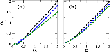
In Fig. 1, we present the parameter $\alpha_{0}$ of the PRBUM ensemble as a function of the parameter $\alpha$ of the initial PRBM ensemble. This result shows that the numerically found values of $\alpha_{0}$ depend on the parameters $\alpha$ and $b$ of the PRBM used in the first step of our algorithm. Moreover, even with the same set of $\alpha$ and $b$, the values of $\alpha_{0}$ for PRBUM-CUE differ from those for PRBUM-COE. For this reason, we still prefer to use the parameters $\alpha$ and $b$ to characterize our PRBUM. Figure 2 depicts the normalized density distribution of the eigenphases for both PRBUM-COE and PRBUM-CUE. Eigenphase $\theta$ of a unitary operator $U$ is defined in the following way:

$$U|\phi_{\lambda}\rangle=\exp(i\theta_{\lambda})|\phi_{\lambda}\rangle,$$ (3)

where $\{|\phi_{\lambda}\rangle\}$ is an eigenstate of $U$. The distribution is found to be uniform as in the CUE and COE cases. Here we show result only for $b=0.1$ with $\alpha=0.5$. For other values of $\alpha$, we also find similar uniform density. This result is important because it indicates that the PRBUM ensemble also satisfies Haar measure and our algorithm is very robust. As such, there is no need to carry out an unfolding procedure when we study the NNSD.

Figure 2: (Color online) Normalized distribution [denoted $\rho(\theta)$] of the eigenphases $\theta$ for (a) PRBUM-COE and for (b) PRBUM-CUE. Here the parameters $b=0.1$, $\alpha=0.5$. The matrix dimension $N=50$ and the ensemble size is 10000. Numerical results here indicate a uniform eigenphase density.

3 Fractal dimension analysis of PRBUM eigenvectors

The fractal statistics of PRBUM eigenvectors can be analyzed by the inverse participation ratio (IPR),

$$P_{2}^{(\lambda)}=\sum_{m}|\langle m|\phi_{\lambda}\rangle|^{4},$$ (4)

where $\lambda$ is the index for eigenstates $|\phi_{\lambda}\rangle$ and $\{|m\rangle\}$ are generic basis states. In our early study JJJ , it was found that for $\alpha=1.0$, the IPR scales anomalously (i.e., $D_{2}$ is fraction) with the Hilbert space dimension $N$, i.e.,

$$P_{2}^{(\lambda)}\sim N^{-D_{2}^{(\lambda)}},$$ (5)

where $D_{2}^{(\lambda)}$ is just the fractal dimension of a particular eigenstate $|\phi_{\lambda}\rangle$. Following the methodology in studies of the PRBM ensemble mirlin1 ; mirlin2 , it was further observed in Ref. JJJ that for sufficiently large $N$, the distribution of $\ln(P_{2}^{(\lambda)})$ for $\alpha=1.0$ displays evidence of being scale-invariant. This scale-invariance, which also suggests self-similarity, is valid upto a certain scale. We define $D_{2}$ in the non-critical regime where, at the thermodynamic limit, the system should be either in delocalized ($D_{2}=1.0$) or localized ($D_{2}=0.0$) regime. However, due to the bounded scale, some part of the delocalized or localized regime (close to the critical point) may show self-similarity like at the critical point with different fractional value of $D_{2}$.

Basically the technique of determining $D_{2}$ is following: due to the scale-invariance, the distribution function of $\ln(P_{2}^{(\lambda)})$ only shifts as $N$ varies. As such the spectral average of $\ln(P_{2}^{(\lambda)})$, denoted by $\langle\ln(P_{2})\rangle$, is linearly related to $\ln N$. The slope of the $\langle\ln(P_{2})\rangle$ vs $\ln N$ curve gives a single fractal dimension $D_{2}$ for the system. The scaling of the variance of $P_{2}^{(\lambda)}$ with $N$ is also studied in Ref. JJJ for $\alpha=1.0$, with features different from those observed in PRBM. We have also observed that conclusions drawn in Ref. JJJ based on PRBUM for $\alpha=1.0$ are also valid if we apply our analysis to a different random unitary matrix model that also aims to describe fractal and intermediate statistics in quantum mapping systems french ; jayendraun .

Figure 3: (Color online) The fractal dimension $D_{2}$ of the eigenvectors of PRBUM plotted as a function of $\alpha$, for $b=0.1({\bullet}),0.3(\blacktriangle)$, and $0.5(\blacksquare)$. For both (a) PRBUM-COE and (b) PRBUM-CUE, one may identify that the delocalization-localization transition occurs around $\alpha=1.0$.

The purpose of this section is twofold. First, we present further numerical evidence that like PRBM, the case of $\alpha=1.0$ is at least (if not exactly) close to the critical transition point of PRBUM. We do so by examining the transition of the fractal dimension $D_{2}$ as a function of $\alpha$ for various values of $b$. Second, we examine the dependence of the fractal dimension $D_{2}$ upon $b$. Note that since we are not in the thermodynamic limit, so the $D_{2}$ values only represent some self-similar properties within a certain scale.

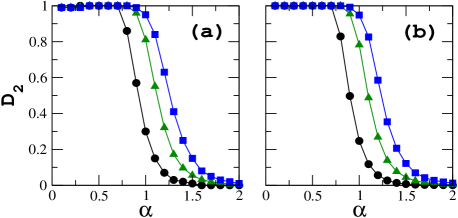
In Fig. 3, we show the dependence of the numerically obtained $D_{2}$ as a function of $\alpha$ for three different values of $b$, i.e., $b=0.1,0.3$ and $0.5$. Similar to Ref. JJJ , we have considered matrix sizes ranging from a few hundreds to a few thousands to extract the value of $D_{2}$. Left and right panels of Fig. 3 are for PRBUM-COE and PRBUM-CUE, respectively. For both cases, as the value of $\alpha$ scans through unity, we have the change from $D_{2}\sim 1.0$ to $D_{2}\sim 0.0$, which reflects the transition from extended states to localized states. This is always the case despite the big change in the values $b$ (see discussion below). In this sense, our PRBUM ensemble may be regarded as another unitary model of the Anderson transition AT_unitary . However, the delocalization-localization transition is not very sharp; eigenstates are fractal ($1.0>D_{2}>0.0$) for a somewhat wide range of values of $\alpha$ around $\alpha=1.0$. We will discuss more on this issue in the next section.

Figure 4: (Color online) The fractal dimension $D_{2}$ of the critical eigenstates of (a) PRBUM-COE and (b) PRBUM-CUE as a function of $b$. For the PRBUM-COE case, in the $b\ll 1$ regime $D_{2}$ varies linearly with $b$ as $D_{2}=3b$ (dashed line). In the regime $b\in[0.2,1.0]$, $D_{2}$ approximately follows $D_{2}=a-c/b$ (solid line) where the parameters $a\simeq 1.11$ and $c\simeq 0.10$. Finally, in the $b\gtrsim 1.0$ regime $D_{2}$ rapidly saturates at a value close to unity (dashed-dot line). For the PRBUM-CUE case, $D_{2}$ behaves qualitatively the same as in the PRBUM-COE case. However, in the $b\ll 1$ regime, $D_{2}$ does not exactly follow $D_{2}=3b$. In the $b\in[0.2,1.0]$ regime, $D_{2}$ again approximately follows $b$ as $D_{2}=a-c/b$ with $a\simeq 1.17$ and $c\simeq 0.12$. The same $D_{2}$ is also plotted as a function of $b_{0}$ for (c) PRBUM-COE and (d) PRBUM-CUE. There, for the PRBUM-COE case and for $b\in[0.01,0.2]$ and hence $b_{0}\in[0.2,0.8]$, $D_{2}\simeq 1.13b_{0}$ (dashed line). In the regime of intermediate $b$ values, we cannot fit $D_{2}$ vs $b_{0}$ curve by the function $D_{2}=a-c/b_{0}$. For even larger $b_{0}$ values, similar fast saturation of $D_{2}$ is observed. The PRBUM-CUE case behaves qualitatively the same.

In Fig. 4(a) and (b) we show how the fractal dimension $D_{2}$ of PRBUM eigenstates for $\alpha=1.0$ depends on $b$. For the PRBUM-COE case, in $b\ll 1$ regime, $D_{2}$ is found to change linearly with $b$, namely, $D_{2}=3b$ (dashed line in Fig. 4(a)). This feature is different from the parallel result from the PRBM ensemble at $\alpha=1.0$, which gives $D_{2}=2b$ mirlin2 . One may wonder if this difference is simply due to the difference between $b$ and $b_{0}$. So in Fig. 4(c), we also show how $D_{2}$ depends on $b_{0}$. Here we like to mention that, when $b$ varies from $0.01$ to $0.2$, correspondingly $b_{0}$ varies from $0.2$ to $0.8$. In this regime, we find $D_{2}\simeq 1.13b_{0}$ (dashed line in Fig. 4(c)), this expression is giving a proportionality constant far from two. For the PRBUM-CUE case, in the same regime, $D_{2}$ still varies linearly with $b$ (dashed line in Fig. 4(b)); but the proportionality constant is not an integer ($D_{2}\simeq 2.68b$). On the other hand, $D_{2}$ varies with $b_{0}$ as $D_{2}\simeq 2.22b_{0}$ (dashed line in Fig. 4(d)). By contrast, in the regime $b\in[0.2,1.0]$, $D_{2}$ approximately follows $b$ as $D_{2}=a-c/b$ (solid line in Fig. 4 (a) and (b)) where $a$ and $c$ are constants. We also find from our numerical fit that, for the PRBUM-COE case $a\simeq 1.11$ and $c\simeq 0.10$; whereas for the PRBUM-CUE case, $a\simeq 1.17$ and $c\simeq 0.12$. This behavior is qualitatively similar to the behavior observed in case of the PRBM ensemble. For PRBM in the same regime, $D_{2}=1-1/\beta\pi b$ where $\beta=1$ and $2$ for the orthogonal and unitary symmetries, respectively mirlin2 . Note also that we cannot get a nice fitting with the same form for the $D_{2}$ vs. $b_{0}$ curve. Furthermore, in the regime of $b\gtrsim 1$, $D_{2}$ is found to rapidly approach a constant value $1-\epsilon$, where $\epsilon\simeq 0.013$ for the PRBUM-COE case and $\epsilon\simeq 0.011$ for the PRBUM-CUE case (dashed-dot line in Fig. 4(a) and (b)). Similar fast saturation of $D_{2}$ to a constant value is also observed in $D_{2}$ vs. $b_{0}$ curve. Results in Fig. 4 also suggest that tuning the $b$ value from $b=0.1$ to $b=0.5$ as in Fig. 3 already covers a significant range.

4 Is $\alpha=1.0$ the transition point?

In the previous section, we have shown that the PRBUM delocalization-localization transition takes place somewhere around $\alpha=1.0$. The exact transition point is not determined. Numerically, similar results were also observed in the case of PRBM. However in the PRBM case, one can analytically determine the exact transition point by mapping the problem onto a nonlinear $\sigma$ model with nonlocal interactions prbm-pap . Because we do not have a good analytical tool for treating PRBUM, we need to rely on numerical investigations. So we now further investigate the transition point from a different perspective.

For PRBM, the ‘not so sharp transition’ was attributed to the fact that there exists a range of values of $\alpha$ around unity in which the eigenstates are fractal up to a characteristic length denoted by $\xi_{\text{frac}}$. This length is anomalously large as compared to the system size and it diverges around $\alpha=1.0$ anom_large_crit . Following the procedure given in Ref. anom_large_crit , we now calculate a different kind of fractal dimension $d_{2}$ of the eigenstates by employing standard box counting procedure through the expression

Figure 5: (Color online) Ensemble average of the fractal dimension $d_{2}$ is calculated using box counting procedure as a function of the system size $N$ for $\alpha=0.80,0.90,0.95,1.00,1.05,1.10$ and $1.20$ from top to bottom. Here we construct the ensemble by taking $1200$ to $300$ matrices for different Hilbert space dimensions. The results for PRBUM-COE and PRBUM-CUE are presented respectively in panel (a) and (b), with $b=0.1$.

Figure 6: Logarithm of the characteristic length $\xi_{\text{frac}}$ (determined from the results in Fig. 5) is plotted as a function of $\alpha$ for (a) PRBUM-COE and (b) PRBUM-CUE. At $\alpha\approx 1.0$, $\log(\xi_{\text{frac}})$ shows signs of divergence.

$$d_{2}\equiv\lim_{\delta\rightarrow 0}\frac{\ln[\chi_{2}(n)]}{\ln\delta}$$ (6)

where $\delta=n/N$ and $\chi_{2}(n)$ is the $2$nd moment of the probability density of the eigenstate in the boxes of size $n$. In the delocalized (metallic) regime, $d_{2}$ should approach towards $1$ from its fractional value as we increase the system size $N$. So in this regime, the slope of $d_{2}$ vs. $N$ curve is expected to be positive. On the other hand, in the localized regime, the limiting value of $d_{2}$ should be $0$, and consequently the slope of the $d_{2}$ vs. $N$ curve will be negative. This implies that there exists a critical value of $\alpha$ at which the slope will be zero. This particular value of $\alpha$ can be regarded as a more precise transition point and on that point $d_{2}$ will be independent of the system size (i.e. scale-invariance), at least for the system size we considered. The characteristic length $\xi_{\text{frac}}$ can be defined as an extrapolated system size for which $d_{2}=1.0$ and $0.0$ in the delocalized and the localized regime, respectively.

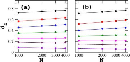
To proceed with this new angle we perform ensemble averages of $d_{2}$ over those eigenstates of a matrix that have IPR values close to the maximal IPR (thus reducing the fluctuations in $d_{2}$). Here we construct the ensemble by taking $1200$ to $300$ matrices depends on the Hilbert space dimension. In Fig. 5, we plot $d_{2}$ as a function of the system size $N$ for $\alpha=0.80,0.90,0.95,1.00,1.05,1.10$ and $1.20$ from top to bottom on a semi-logarithmic scale. The results therein can be regarded as a type of finite-size scaling analysis (quite different from other approaches, e.g., finite-size ). These curves are fitted very well by straight lines. We then determine $\log(\xi_{\text{frac}})$ as a function of $\alpha$ from these fitted straight lines. The results are presented in Fig. 6. For both panels in Fig. 6, the left (right) part of $\log(\xi_{\text{frac}})$ vs $\alpha$ curve shows the fitted results using $d_{2}=1$ ($d_{2}=0$). Similar to the PRBM ensemble case anom_large_crit , we can see that $\log(\xi_{\text{frac}})$ diverges around $\alpha=1.0$.

Figure 7: (Color online) The slope $\eta$ of $d_{2}$ vs. $\log(N)$ curves (as presented in Fig. 5) is plotted as a function of $\alpha$ for (a) PRBUM-COE and (b) PRBUM-CUE. These results are fitted with a linear function (solid line) which gives slope $p=0.76$ and intercept $q=0.72$ for the PRBUM-COE case. For the PRBUM-CUE case, the slope $p=0.73$ and the intercept $q=0.77$. In both panels, the horizontal line represents $\eta=0$ and the vertical line indicates $\alpha=1.0$.

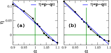
In Fig. 7, we plot the slope $\eta$ determined from the $d_{2}$ vs. $N$ curves in Fig. 5, for different values of $\alpha$. The presented results suggest that, at $\alpha=1.0$, $\eta$ is approximately equal to $0.05$. This slope is small, but not exactly zero. The slope reaches nearest to zero around $\alpha=1.05$. In this sense, $\alpha=1.05$ may be regarded as a more precise transition point for both PRBUM-COE and PRBUM-CUE cases (applies to $b=1.0$ as well). One may suspect that, instead of $\alpha=1.0$, $\alpha_{0}=1.0$ might be the precise transition point. However, according to Fig. 1, at $\alpha=1.05$, the parameter $\alpha_{0}$ is approximately equal to $0.95$. So we have to rule out this possibility. Another interesting observation from Fig. 7 is the following: around $\alpha=1.0$, the slope $\eta$ is essentially a linear function of $\alpha$. The corresponding linear fitting of the form $\eta=p-q\alpha$ gives $p\simeq 0.76$ and $q\simeq 0.72$ for the PRBUM-COE case, and $p\simeq 0.73$ and $q\simeq 0.77$ for the PRBUM-CUE case. In both cases, $p\approx q$. If we assume $p=q$ in the thermodynamic limit, then $\eta\simeq p(1-\alpha)$, which predicts that $\eta$ is zero only when $\alpha=1.0$. This hints that even here $\alpha=1.05$ seems to be the more precise critical point for $b=0.1$, the slight departure from $\alpha=1.0$ can be due to the finite size of our system. One can also use our PRBUM algorithm to argue in favor of $\alpha=1.0$ as the true transition point in the thermodynamics limit. That is, if $\alpha=1.0$ is not the transition point, then our algorithm would have to generate a critical PRBUM ensemble starting from a non-critical PRBM ensemble.

5 Statistics of PRBUM eigenvector components

Figure 8: (Color online) Typical eigenvector profile for PRBUM-COE [(a)-(c)] and PRBUM-CUE [(d)-(f)]. In (a) and (d) $\alpha=0.5$; in (b) and (e) $\alpha=1.0$, and in (c) and (f) $\alpha=1.5$. $b=0.1$ is fixed.

In this section we investigate the statistical properties of the eigenvector components of PRBUM. This is interesting because the parallel results for standard Dyson’s circular ensembles provide a good reference point for us. Figure 8 depicts the profile of some typical eigenvectors for PRBUM-COE and PRBUM-CUE, for three different values of $\alpha$, i.e., $\alpha=0.5,1.0,$ and $1.5$, and a fixed $b$ value. For $\alpha=0.5$ shown in Fig. 8(a) and Fig. 8(d), both PRBUM-COE and PRBUM-CUE give delocalized random eigenvectors, which is consistent with the observation that $D_{2}\sim 1$ for $\alpha=0.5$. Turning to Fig. 8(b) and Fig. 8(e) for the case of $\alpha=1.0$, the eigenvectors exhibit a quite sparse structure, but are not localized in any particular regime. The same property was observed in the PRBM ensemble prbm-pap . Finally, for the case of $\alpha=1.5$ shown in Fig. 8(c) and Fig. 8(f), it is seen that the eigenvectors are highly localized, which is consistent with the result of $D_{2}\sim 0$ seen in Fig. 3. In the following we discuss the statistics of the magnitude of PRBUM eigenvector components.

Figure 9: (Color online) Distribution function $P(z)$ vs $z$ for the eigenvector component statistics of PRBUM-COE, where $z=\ln[N|\langle m|\phi_{\lambda}\rangle|^{2}]$ and $N$ is the matrix size. Here $N=500$ and $b=0.1$. (a) $\alpha=0.1$, the solid line represents the standard COE distribution of Eq. (8). (b) Same as in (a) but with $\alpha=0.5$. (c) $\alpha=1.0$ (around the critical point). The central part of $P(z)$ follows closely a normal distribution (solid line) with mean value $\langle z\rangle\simeq-5.34$, and variance $\sigma_{z}\simeq 3.25$. Strong deviations from the normal distribution are seen for $|z|\gg 0$. (d) $\alpha=1.5$. An additional peak (location indicated by the vertical solid line) appears at $z=\ln N=\ln(500)\simeq 6.22$. This additional peak is due to the emergence of some most localized states.

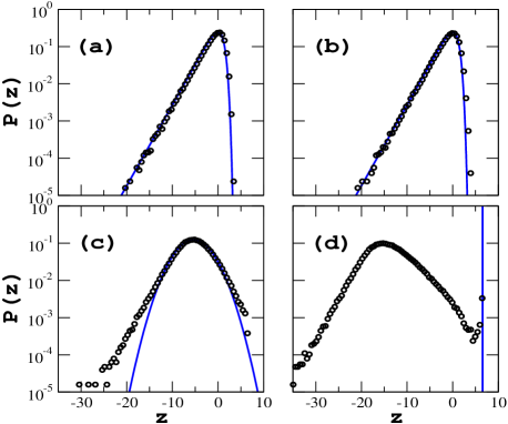
Figure 9 shows the distribution function of the magnitude squared of the eigenvector components for PRBUM-COE, considering an ensemble of $100$ matrices with $N=500$, for four different $\alpha$ values but with the $b$ value fixed at $b=0.1$. The results are plotted in terms of the probability distribution function $P(z)$, where $z\equiv\ln y\equiv\ln[N|\langle m|\phi_{\lambda}\rangle|^{2}]$. In the case of $\alpha=0.1$, because the associated fractal dimensional $D_{2}\sim 1.0$ (see Fig. 3), one expects $P(z)$ to follow Dyson’s standard COE distribution for eigenvector components. Because the COE distribution of $y$ is given by porter

$$p(y)=\frac{1}{\sqrt{2\pi y}}\exp\left(-\frac{y}{2}\right),$$ (7)

the COE distribution for $z$ is given by

$$P_{\text{COE}}(z)=\frac{1}{\sqrt{2\pi}}\exp\left[\frac{z-\exp(z)}{2}\right].$$ (8)

As seen in Fig. 9(a), the numerical result (open circle) follows Eq. (8) (solid line) remarkably well. The value of $\alpha$ is then increased to $\alpha=0.5$ in Fig. 9(b). It is found that $P(z)$ is still very close to $P_{\text{COE}}(z)$, with slight deviation at the right tail. This is consistent with our early observation that the $D_{2}$ value is still close to unity for $\alpha=0.5$. The case $\alpha=1.0$ is shown in Fig. 9(c), where $P(z)$ is seen to be significantly different from the COE distribution $P_{\text{COE}}(z)$. Indeed, the $P(z)$ for PRBUM-COE for this (at least) near-critical case is much broader than $P_{\text{COE}}(z)$, reflecting that the possibility of having very large or very small eigenvector components is much higher than in the conventional random matrix theory. The solid line in Fig. 9(c) represents a normal distribution, and it is seen that the central part of $P(z)$ is close to the normal distribution. Finally, Fig. 9(d) displays the result for $\alpha=1.5$, a value that yields $D_{2}\rightarrow 0$ as seen in Fig. 3. In this case, many eigenvectors are highly localized and as a result, one observes a much enhanced probability at large $z$. Indeed, because the most localized eigenvector has only one component with magnitude unity and all other components with magnitude zero, it is now possible to have a high probability at $z=\ln N$. The additional peak at $z=\ln 500\simeq 6.22$ in Fig. 9(d) indicates that some of the eigenstates are actually close to the most localized states. We have also checked that if $\alpha$ further increases, then this additional peak becomes more and more pronounced. At about $\alpha=10.0$ essentially all the eigenvectors become the most localized states.

Figure 10: (Color online) Same as in Fig. 9, but for PRBUM-CUE. (a) $\alpha=0.1$. The solid line represents the standard CUE distribution given in Eq. (10). (b) Same as (a) but for $\alpha=0.5$. (c) $\alpha=1.0$ (around the critical point). $P(z)$ follows closely a normal distribution (solid line) with mean $\langle z\rangle\simeq-5.93$ and variance $\sigma_{z}\simeq 2.95$. Strong deviations from the normal distribution are seen for $z\gg 0$. The left tail ($P(z)$ at $z\ll 0$) agrees with the normal distribution better than in the PRBUM-COE case. (d) $\alpha=1.5$. An additional peak (location indicated by the vertical solid line) appears at $z=\ln N=\ln(500)\simeq 6.22$. This additional peak is due to the emergence of some most localized states.

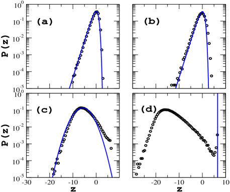
Let us now perform the same analysis for PRBUM-CUE and the results are presented in Fig. 10. Here the reference point is Dyson’s CUE statistics of the magnitude squared of eigenvector components porter , i.e.,

$$p(y)=\exp(-y),$$ (9)

which leads to

$$P_{\text{CUE}}(z)=\exp\left[z-\exp(z)\right].$$ (10)

As seen from Fig. 10(a), the numerical result for $\alpha=0.1$ agrees with $P_{\text{CUE}}(z)$ for the entire range of $z$. This again confirms that PRBUM essentially reduces to CUE for a sufficient small $\alpha$. In the case $\alpha=0.5$ shown in Fig. 10(b), $P(z)$ closely follows $P_{\text{CUE}}(z)$ with marginal deviation in the right tail. The case of $\alpha=1.0$ in the delocalization-localization transition regime is shown in Fig. 10(c), with features clearly different from that of $P_{\text{CUE}}(z)$. We have also compared the numerical result with a normal distribution [solid line in Fig. 10(c)]. Interestingly, the left part of $P(z)$ as well as its central part is seen to agree with the fitted normal distribution reasonably well, but clear deviation from the normal distribution is seen for $z\gg 0$. This feature is different from what is observed in the PRBUM-COE case [see Fig. 9(c)], where deviations from a normal distribution is also clearly seen in the left tail. The result for $\alpha=1.5$ is shown in Fig. 10(d). Similar to the PRBUM-COE case in Fig. 9(d), here again an additional peak emerges at $z=\ln(500)\simeq 6.22$, which is clear evidence that some states become the most localized states.

Summarizing this section, it is observed that when the delocalization-localization transition occurs, the distribution function $P(z)$ for PRBUM shows strong deviations from Dyson’s COE/CUE predictions. These deviations may be regarded as one main characteristic of the Anderson transition. Interestingly, in the case of PRBUM-CUE, both the central part and the left tail of $P(z)$ is close to a normal distribution, whereas in the case of PRBUM-COE, only the central part of $P(z)$ is close to a normal distribution.

6 Critical spectral behavior of PRBUM

In this section we investigate the manifestations of the delocalization-localization transition of PRBUM in its NNSD statistics. In the Anderson tight-binding model on a $3D$ cubic lattice, Braun et al. found that on the metal-insulator transition point, the NNSD depends on the boundary conditions of the cubic lattice braun1 . Upon averaging over different boundary conditions, it was discovered that the NNSD follows approximately the semi-Poisson distribution, i.e.,

$$P_{\text{sp}}(s)=4s\exp(-2s),$$ (11)

where $s\geq 0$ is the spacing between two neighboring levels. In the $s\rightarrow 0$ limit, $P_{\text{sp}}(s)\sim 4s$, which is a linear level repulsion property shared by Dyson’s COE statistics and many time-reversal symmetric dynamical systems with chaotic classical limits mehta ; haakebook . However, the proportionality constant in the linear level repulsion for $P_{\text{sp}}(s)\sim 4s$ is different from Dyson’s COE statistics $P_{\text{COE}}(s)\sim\frac{\pi}{2}s$. In the other limit $s\gg 0$, $P_{\text{sp}}(s)$ decays exponentially, i.e., $P_{\text{sp}}(s)\sim\exp(-2s)$, which is reminiscent of an uncorrelated energy spectrum of a regular quantum system whose NNSD follows the Poisson distribution $P_{\text{p}}(s)=\exp(-s)$. Hence in this second limit $P_{\text{sp}}(s)$ differs significantly from $P_{\text{COE}}(s)$ which decays to zero as $\exp(-\pi s^{2}/4)$. Therefore, the semi-Poisson distribution $P_{\text{sp}}(s)$ can be considered as an intermediate critical NNSD behavior. In Ref. braun2 , the NNSD of the PRBM ensemble was also studied. The finding is that the central part of the NNSD follows $P_{\text{sp}}(s)$ well, but non-negligible deviations from $P_{\text{sp}}(s)$ were observed for $s\rightarrow 0$ or for $s\gg 0$ regime. We are thus motivated to carry out similar NNSD studies for PRBUM in the Anderson transition regime and also use the semi-Poisson distribution as one of our diagnostic tools. Note also that, since Fig. 2 already confirms the uniform distribution of PRBUM eigenphases, we only need to introduce a simple re-scaling factor $N/2\pi$ to set the average level spacing at unity.

Figure 11: (Color online) The NNSD [denoted $P(s)$] of the eigenphases of PRBUM-COE (open circles) vs level spacing $s$, for four different values of $\alpha$. For the sake of comparison, the Wigner-Dyson distribution for COE (dashed line), the semi-Poisson distribution as given in Eq.(11) (solid line), and the Poisson distribution (dashed-dotted line) are all plotted together. (a) $\alpha=0.1$. (b) $\alpha=0.5$. (c) $\alpha=1.0$. (d) $\alpha=1.5$. An ensemble of 100 matrices with $N=1000$ is used for statistics. Results here should be connected with those in Fig. 9.

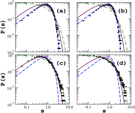
For the same four PRBUM-COE cases as in Fig. 9, Fig. 11 depicts the associated NNSD. In case of $\alpha=0.1$ in Fig. 11(a), the numerically obtained NNSD (denoted by $P(s)$ and represented by open circles) is in good agreement with the Wigner-Dyson statistics $P_{\text{COE}}(s)$ from the conventional random matrix theory (dashed line). For the sake of comparison, in all the four figure panels we have plotted the semi-Poisson distribution $P_{\text{sp}}(s)$ (solid line) as given in Eq. (11) as well as the Poisson distribution $P_{p}(s)$ (dashed-dotted line). The case of $\alpha=0.5$ in Fig. 11(b) is similar. Consider next the critical case in Fig. 11(c). Quite unexpectedly, $P(s)$ follows the semi-Poisson distribution $P_{\text{sp}}(s)$ very well in the small-$s$ regime. This agreement in the small-$s$ regime is absent in PRBM on the critical point. In the large-$s$ regime, deviations from the semi-Poisson distribution can be seen clearly in Fig. 11(c). Indeed, $P(s)$ in the large-$s$ regime is seen to lie between the semi-Poisson distribution and the Poisson distribution. This feature is also different from one case study of the $P(s)$ of PRBM braun2 . In particular, in Ref. braun2 the $P(s)$ for PRBM actually lies between $P_{\text{COE}}(s)$ and $P_{\text{sp}}(s)$, instead of between $P_{\text{sp}}(s)$ and $P_{\text{p}}(s)$. This difference can be explained as follows. For $b=1.0$ considered in Ref. braun2 , the fractal dimension of PRBM eigenstates is $D_{2}\simeq 0.66$; whereas here $b=0.1$ and $D_{2}\sim 0.28$. As such, the $D_{2}$ value in Ref. braun2 is closer to unity and the NNSD result is expected to be closer to the conventional random matrix theory. Furthermore, the much smaller $D_{2}$ value for our PRBUM considered here should imply more localized states, and hence the $P(s)$ is closer to the Poisson distribution. Consistent with this explanation, the case of $\alpha=1.5$ in Fig. 8(d) has $D_{2}\sim 0$, and the associated $P(s)$ indeed agrees well with the Poisson distribution (dashed-dot line).

Figure 12: (Color online) Same as in Fig. 11, but for PRBUM-CUE. Here the dashed line represents the Wigner-Dyson distribution for CUE, and the dotted line represents the generalized semi-Poisson distribution given in Eq. (12) with $\beta=2.0$. The dashed-dotted line is still for the Poisson distribution and and the solid line is still for the semi-Poisson distribution. An ensemble of 100 matrices with $N=1000$ is used for statistics. Results here should be compared with those in Fig. 10.

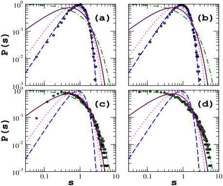
We next examine the NNSD for PRBUM-CUE in Fig. 12. The standard Wigner-Dyson distribution for CUE with quadratic level repulsion is now plotted as dashed lines in all the four panels. As expected, $P(s)$ in the cases of $\alpha=0.1$ and $\alpha=0.5$ in Fig. 12(a) and Fig. 12(b) agree with the standard result from random matrix theory. Similarly, Fig. 12(d) shows that $P(s)$ for PRBUM-CUE follows the Poisson distribution for $\alpha=1.5$, indicating that this $\alpha$ value is far beyond the delocalization-localization transition point. Much more interesting is the case of $\alpha=1.0$. Similar to the PRBUM-COE case, in the large-$s$ regime $P(s)$ is found to lie between the semi-Poisson distribution and the Poisson distribution. For the small-$s$ regime, since $P(s)$ in the PRBUM-COE case nicely follows a semi-Poisson distribution, one might naively expect that here, due to the breaking of time-reversal symmetry, the $P(s)$ should follow a generalized semi-Poisson distribution bogomolny with quadratic level repulsion. To check if this expectation is correct, in all the panels of Fig. 12 we have plotted an additional curve (dotted line) to represent a generalized semi-Poisson distribution $P_{\text{sp};\beta}(s)$ with $\beta=2$, i.e.,

$$P_{\text{sp};\beta}(s)=A_{\beta}s^{\beta}\exp[-(\beta+1)s],~{}~{}A_{\beta}=\frac{(\beta+1)^{\beta+1}}{\Gamma(\beta+1)}.$$ (12)

Note that $P_{\text{sp};\beta=1}(s)=P_{\text{sp}}(s)$. As seen in Fig. 12(c), in the small-$s$ regime, the $P(s)$ for PRBUM-CUE deviates from both $P_{\text{sp};\beta}(s)$ with $\beta=2$ and the semi-Poisson distribution $P_{\text{sp}}(s)$. This implies the possibility of anomalous level repulsion, namely, $P(s)\sim s^{\beta}$ with $\beta$ being a non-integer.

Figure 13: (Color online) The NNSD [denoted $P(s)$] and the integrated nearest neighbor spacing statistics [denoted $I(s)$] in the small-$s$ regime for both PRBUM-COE and PRBUM-CUE. In the top two panels, the numerical data (open circles) are fitted by $P(s)\sim s^{\beta}$. In the case of PRBUM-COE, $\beta\simeq 1.04$ (almost linear repulsion), whereas in the case of PRBUM-CUE, $\beta\simeq 1.73$ (signature of anomalous level repulsion). For the bottom two panels, $I(s)$ vs $s$ is fitted by $I(s)\sim s^{\beta^{\prime}}$, with $\beta^{\prime}\simeq 2.01$ for PRBUM-COE and $\beta^{\prime}\simeq 2.71$ for PRBUM-CUE, thereby further confirming the found $\beta$ values. To improve the statistics in the small-$s$ regime, an ensemble of 1000 matrices with $N=1000$ is used for our statistics.

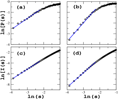
In order to investigate carefully the anomalous level repulsion for critical PRBUM-CUE in the small-$s$ regime, we show in Fig. 13 the $\ln[P(s)]$ vs. $\ln(s)$ plot in the small-$s$ regime ($s<0.36$) and then fit it using the function $P(s)\sim s^{\beta}$. To show the marked difference between PRBUM-CUE and PRBUM-COE around the critical point, this fitting is also performed for PRBUM-COE. We obtain $\beta\simeq 1.04$ for PRBUM-COE, which confirms the linear level repulsion observed earlier in Fig. 11. By contrast, for PRBUM-CUE, we find $\beta\simeq 1.73$, clear evidence of anomalous level repulsion. To improve the statistics in the small-$s$ regime, we increased the ensemble size by a factor of ten, i.e., now an ensemble of 1000 matrices with $N=1000$ is used for our statistics. We have further checked that the change in the $\beta$ values thus found numerically is negligible if we further increase the ensemble size by a factor of three. Thus, at least for the small-$s$ regime we considered, the level repulsion is found to be anomalous. In the bottom two panels of Fig. 13, the numerical fitting of the integrated nearest-neighbor spacing distribution, denoted by $I(s)$, is also presented. The fitting curve $I(s)\sim s^{\beta^{\prime}}$ yields $\beta^{\prime}\simeq 2.01$ for PRBUM-COE and $\beta^{\prime}\simeq 2.71$ for PRBUM-CUE [Note that, by definition of $I(s)$, $\beta^{\prime}=\beta+1$]. This further supports our earlier observation that $P(s)$ displays an anomalous level repulsion in the case of PRBUM-CUE.

7 Concluding remarks

The Hermitian PRBM ensemble has been studied extensively in the literature as a standard model for the Anderson transition. In terms of the power-law decay of the magnitude of the matrix elements from the diagonal, the unitary PRBUM ensemble is similar to PRBM (the generation of PRBUM is much more involved). This work showed that, statistics of PRBUM in the delocalization-localization transition regime can be different from their PRBM counterparts. Hence PRBUM is not a trivial unitary analog of the Hermitian PRBM ensemble. Somewhat consistent with this conclusion, we have observed that for a given set of $b$ and $\alpha$, the matrix elements of PRBUM as generated from our algorithm decay from the diagonal as a different power-law function [see Eq. (2) and Fig. 1, where $b_{0}$ and $\alpha_{0}$ can be appreciably different from $b$ and $\alpha$]. Given our detailed findings, we hope that PRBUM can capture some critical behavior of actual Floquet eigenstates in the delocalization-localization transition regime, by modeling system’s periodic unitary evolution matrix with power-law decaying matrix elements. Different choices of ensemble parameters can model a system in either insulating or metallic phase, and if the ensemble parameters are close to critical values, then fractal behavior of the Floquet eigenstates (within a certain scale) may be also modeled by PRBUM. One obvious advantage of PRBUM as compared with PRBM is that in performing the statistics all the eigenstates are treated under equal footing, rather than selecting certain energy windows as often done in PRBM studies. We also note that in our early study JJJ PRBUM can correctly model how the variance of $D_{2}$ of Floquet eigenstates (in a double-kicked top model) scales with the system size but PRBM cannot.

In summary, we have numerically studied the statistical properties of PRBUM in the delocalization-localization regime and have compared them with PRBM and the standard random matrix theory when feasible. The dependence of the fractal dimension of PRBUM eigenvectors upon ensemble parameters is used to examine where the delocalization-localization transition point is, within some uncertainty due to finite-size effects. For cases very close to the transition point, the central part of the PRBUM eigenvector-component distribution function is close to a log-normal distribution and the tails (especially the PRBUM-COE case) show strong deviations from the log-normal distribution. We have also examined the NNSD of PRBUM and have compared the result with the semi-Poission distribution and a generalized semi-Poisson distribution. An anomalous level repulsion of PRBUM in the absence of time-reversal symmetry is also numerically found.

This work was supported by the Academic Research Fund Tier I, Ministry of Education, Singapore (grant No. R-144-000-276-112).

References

- (1) M. L. Mehta, Random Matrices, 3rd Ed. (Elsevier, San Diego, 2004).
- (2) C. E. Porter in Statistical Theories of Spectra : Fluctuations, edited by C. E. Porter (Academic, New York, 1965).
- (3) Mesoscopic Phenomena in Solids, edited by B. L. Altshuler et. al. (Elsevier, Amsterdam, 1991).
- (4) H. S. Camarda and P. D. Georgopulos, Phys. Rev. Lett. 50, 492 (1983).
- (5) See, for example, V. Plerou et. al., Phys. Rev. Lett. 83, 1471 (1999); L. Laloux et. al., Phys. Rev. Lett. 83, 1467 (1999).
- (6) M. S. Santhanam and P. K. Patra, Phys. Rev. E 64, 016102 (2001).
- (7) P. Seba, Phys. Rev. Lett. 91, 198104 (2003).
- (8) See for examples : S. N. Dorogovtsev et. al. Phys. Rev. E 68, 046109 (2003); J. N. Bandyopadhyay and S. Jalan, Phys. Rev. E 76, 026109 (2007); S. Jalan and J. N. Bandyopadhyay, Phys. Rev. E 76, 046107 (2007).
- (9) See, for example, P. Shukla, Phys. Rev. E 75, 051113 (2007); P. Shukla, Phys. Rev. Lett. 87, 194102 (2001).
- (10) F. Haake, Quantum Signatures of Chaos (Springer-Verlag, New York, 1992).
- (11) L. E. Reichl, The Transition to Chaos: Conservative Classical Systems and Quantum Manifestations (Springer-Verlag, New York, 1992).
- (12) O. Bohigas, M. J. Giannoni, and C. Schmit, Phys. Rev. Lett. 52, 1 (1984).
- (13) M. V. Berry and M. Tabor, Proc. R. Soc. A 356, 375 (1977).
- (14) P. W. Anderson, Phys. Rev. 109, 1492 (1958).
- (15) F. Evers and A. D. Mirlin, Rev. Mod. Phys. 80, 1355 (2008).
- (16) J. Billy et al., Nature (London) 453, 891 (2008).
- (17) G. Lemarié, H. Lignier, D. Delande, P. Szriftgiser, and J. C. Garreau, Phys. Rev. Lett. 105, 090601 (2010).
- (18) B. I. Shklovskii et al., Phys. Rev. B 47, 11487 (1993).
- (19) A. D. Mirlin et al., Phys. Rev. E 54, 3221 (1996).
- (20) P. G. Harper, Proc. of Phys. Soc. London, Sec. A 68, 874 (1955); 68, 879 (1955).
- (21) K. Drese and M. Holthaus, Phys. Rev. Lett. 78, 2932 (1997).
- (22) G. Casati, I. Guarneri, and D. L. Shepelyansky, Phys. Rev. Lett. 62, 345 (1989).
- (23) J. Wang and A. M. García-García, Phys. Rev. E 79, 036206 (2009); A. M. García-García and J. Wang, Phys. Rev. Lett. 94, 244102 (2005).
- (24) For example, T. Geisel, R. Ketzmerick, and G. Petschel, Phys. Rev. Lett. 67, 3635 (1991); R. Artuso, F. Borgonovi, I. Guarneri, L. Rebuzzini, and G. Casati, Phys. Rev. Lett. 69, 3302 (1992).
- (25) J. Wang and J. B. Gong, Phys. Rev. A 77, 031405(R) (2008); W. Lawton, A. S. Mouritzen, J. Wang, and J. B. Gong, J. Math. Phys. 50, 032103 (2009); J. Wang, A. S. Mouritzen, and J. B. Gong, J. Mod. Opt. 56, 722 (2009).
- (26) J. Wang and J. B. Gong, Phys. Rev. Lett. 102, 244102 (2009); Phys. Rev. E 81, 026204 (2010).
- (27) J. N. Bandyopadhyay, J. Wang, and J. B. Gong, Phys. Rev. E 81, 066212 (2010).
- (28) F. J. Dyson, J. Math. Phys. 3, 140 (1962).
- (29) K. C. Hegewisch and S. Tomsovic, EPL 97, 34002, (2012).
- (30) K. Źyczkowski and M. Kus, J. Phys. A 27, 4235 (1994).
- (31) F. Mezzadri, Notices of the AMS 54, 592 (2007).
- (32) Y. V. Fyodorov and A. D. Mirlin, Phys. Rev. B 51, 13403 (1995); F. Evers and A. D. Mirlin, Phys. Rev. Lett. 84, 3690 (2000).
- (33) A. D. Mirlin and F. Evers, Phys. Rev. B 62, 7920 (2000).
- (34) J. Martin, O. Giraud, and B. George, Phys. Rev. E 77, 035201(R) (2008).
- (35) J. N. Bandyopadhyay, unpublished.
- (36) E. Hamza, A. Joye, and G. Stolz, Lett. Math. Phys. 75, 255 (2006); Math. Phys. Anal. Geom. 12, 381 (2009).
- (37) E. Cuevas, V. Gasparian, and M. Ortunõ, Phys. Rev. Lett. 87, 056601 (2001).
- (38) K. Yakubo and M. Ono, Phys. Rev. B 58, 9767 (1998); A. Rodriguez, L. J. Vasquez, K. Slevin, and R. A. Römer, Phys. Rev. Lett. 105, 046403 (2010).
- (39) D. Braun, G. Montambaux, and M. Pascaud, Phys. Rev. Lett. 81, 1062 (1998).
- (40) I. Varga and D. Braun, Phys. Rev. B 61, 11859(R) (2000).
- (41) E. Bogomolny and C. Schmit, Phys. Rev. Lett. 93, 254102 (2002).