Seeded Graph Matching

Abstract

Given two graphs, the graph matching problem is to align the two vertex sets so as to minimize the number of adjacency disagreements between the two graphs. The seeded graph matching problem is the graph matching problem when we are first given a partial alignment that we are tasked with completing. In this article, we modify the state-of-the-art approximate graph matching algorithm “FAQ” of Vogelstein et al. (2015) to make it a fast approximate seeded graph matching algorithm, adapt its applicability to include graphs with differently sized vertex sets, and extend the algorithm so as to provide, for each individual vertex, a nomination list of likely matches. We demonstrate the effectiveness of our algorithm via simulation and real data experiments; indeed, knowledge of even a few seeds can be extremely effective when our seeded graph matching algorithm is used to recover a naturally existing alignment that is only partially observed.

Keywords: Hungarian Algorithm, Quadratic Assignment Problem (QAP), Vertex Alignment.

1 Introduction

It is increasingly common in many scientific disciplines to represent the complex interactions amongst data points via networks, and the statistical and scientific literature has seen a vast amount of work on the modeling and analysis of this burgeoning network data. Often when working simultaneously with multiple graphs, there is a need to register vertices to each other across networks. This data processing step, which is often referred to as graph matching, allows for the application of techniques that use the common, shared labels across networks as known parameters in subsequent inference. As such, the field of graph matching has been the subject of a vast amount of literature in many diverse fields such as pattern recognition [1, 2, 3], computer vision [4, 5, 6], social network analysis [7, 8], and neuroscience [9, 10], to name a few; see the following surveys for a comprehensive overview of the many recent results, advances, and applications of graph matching: “Thirty Years of Graph Matching in Pattern Recognition” by Conte et al (2004) [11], “Graph Matching and Learning in Pattern Recognition in the Last 10 Years” by Foggia et al (2014) [12], and “A Short Survey of Recent Advances in Graph Matching” by Yan et al (2016) [13].

Informally, given two graphs of the same order, the graph matching problem seeks a bijection between the vertex sets of the two graphs that best preserves the adjacency structure across networks. More formally, suppose we are given two graphs, $G_{1}$ and $G_{2}$, with respective vertex sets $V_{1}$ and $V_{2}$ such that $|V_{1}|=|V_{2}|$, where $|V|$ denotes the cardinality of $V$. For any bijective function $\phi:V_{1}\rightarrow V_{2}$, two vertices $u,v\in V_{1}$ are said to have an adjacency disagreement under $\phi$ if $u$ and $v$ are adjacent in $G_{1}$ but $\phi(u)$ and $\phi(v)$ are not adjacent in $G_{2}$, or vice versa. The graph matching problem has as its objective the minimization of the number of adjacency disagreements induced by $\phi$ over all bijective functions $\phi:V_{1}\rightarrow V_{2}$. In its most general form, the graph matching problem is equivalent to the NP-hard quadratic assignment problem [14]. In fact, even the simpler problem of deciding whether there exists a graph isomorphism, while shown to be of subexponential complexity in [15], is not known to be solvable in polynomial time and remains intractable, in general, for large networks. Indeed, there are no known efficient algorithms for graph matching in general, and the consensus is that none exist.

A natural question stemming from graph matching is: What if part of the matching is fixed? Exploration of this seeded graph matching problem is addressed in a number of settings. The authors of [16] and [17] incorporate constraints that enforce correspondences to be only between vertices of the same “type,” and more recent advances include: use in semisupervised learning, spectral clustering, and seed-selection processes (see [18, 19, 20] respectively), exploration of other methods for using seeds in graph matching (see [21, 22]), along with a few surveys covering seeded graph matching (see, for example, [12, 13]).

In the notation introduced above, the seeded graph matching problem can be formulated as follows. Suppose that we are also given subsets $W_{1}\subset V_{1}$, $W_{2}\subset V_{2}$ such that $|W_{1}|=|W_{2}|$, and a fixed bijection $\psi:W_{1}\rightarrow W_{2}$. The seeded graph matching problem is defined to be the problem of minimizing the number of adjacency disagreements induced by $\phi$ over all bijections $\phi:V_{1}\rightarrow V_{2}$ that are extensions of $\psi$ — that is, $\phi$ must agree with $\psi$ on $W_{1}$ (i.e., for all $u\in W_{1}$, $\phi(u)=\psi(u)$). The elements of $W_{1}$ and $W_{2}$ are called seeds and $\psi$ is called a seeding.

In many applications when considering two networks, there is a natural correspondence between the two vertex sets; for example, when looking at an email network and a social network with the same participants, we might say that a vertex in the email network corresponds to a vertex in the social network if the two represent the same participant. In this case, a goal of graph matching would be to recover this natural correspondence if it is unknown. We can therefore consider the seeded graph matching problem as an attempt to recover an underlying vertex correspondence when only a few of these correspondences (seeds with the seeding function) are known a priori. Knowledge of these seeds can yield a dramatic improvement in approximating the natural correspondence, as will be illustrated later in this article.

The purpose of this article is to modify the Fast Approximate Quadratic Assignment Problem (FAQ) graph matching algorithm of Vogelstein et al (2015) [23], so as to

1. Employ the use of seeds — we call this the Seeded Graph Matching Algorithm “SGM”, and

2. Adapt the use of the SGM algorithm to match graphs which have differently sized vertex sets, and

3. Extend the SGM algorithm to provide each vertex with a probability distribution over potential matches.

The modification of FAQ to use seeds (“1” above) was first introduced in the technical report which was an early version of this article. As such, this article has already been a stepping stone from which numerous articles have already been written, all citing this article, including [24, 25, 19, 26, 27, 9, 28, 29, 30].

The motivation for specifically extending the FAQ algorithm comes from the fact that the algorithm is both fast and accurate, and also has strong theoretical justification. Indeed, in Vogelstein et al. (2015) [23] it is shown that the FAQ algorithm is more accurate than the other graph matching algorithms with which it was compared on $94\%$ of the QAPLIB [31] benchmark problems considered. Also, FAQ was faster than the popular PATH algorithm introduced in [32, 33]. Furthermore, from a theoretical standpoint, it is shown in [29] that, under mild conditions, the FAQ algorithm asymptotically almost surely provides the optimal graph matching solution when solved exactly, in contrast to many of the existing alternative problem formulations/solutions.

As mentioned in “2” above, another purpose of this manuscript is to include an extension of graph matching to settings where the vertex sets differ in size; here the goal is to recover a correspondence between the vertices of the smaller graph and a subset of the vertices of the larger graph. Another purpose of this manuscript (“3” above) is to provide, for each vertex, a probability distribution over potential matches. This allows (among other things) for ranking of possible matches, rather than just providing a single proposed match. In particular, by providing each vertex with a ranked list of candidate matching vertices, a practitioner is given a principled means with which to search for the true match for a given vertex, namely, to search the rank list in decreasing likelihood of matching.

In particular, our SGM algorithm would be appropriate to use when two graphs are isomorphic and we seek the isomorphism, and also when two graphs are not isomorphic, and we seek the bijection between the their respective vertex sets that is “closest” to an isomorphism. Furthermore, by Contribution “2” listed above, SGM would be appropriate to use when the graphs have differently sized vertex sets, say $G_{1}$ has fewer vertices than $G_{2}$, and we seek the one-to-one injection from the vertex set of $G_{1}$ into the vertex set of $G_{2}$ which provides the “closest” isomorphic-to-$G_{1}$ induced subgraph of $G_{2}$. All of these tasks could be used to find a natural, underlying correspondence between the vertex sets. Also, by Contribution “3” listed above, SGM would be appropriate to use when we don’t just want a single bijection between the vertex sets, but seek backup, alternative possibilities for natural correspondence to each vertex.

The structure of this paper is as follows: In Section 1.1 we provide the mathematical framework and notation. In Section 2, we describe the graph matching algorithm FAQ of Vogelstein et al (2015) [23] and adapt it into our SGM algorithm for seeded graph matching. We then present an extension of the SGM algorithm for use on graphs having differently sized vertex sets in Section 2.5 and, in Section 2.6, we present a version of the SGM algorithm which outputs, for each pair of nodes in $V_{1}\times V_{2}$, a confidence of being a match across the two graphs. Following, in Section 3 we demonstrate the effectiveness of the SGM algorithm via three real data experiments, and in Section 4 we compare SGM to a seeded version of the PATH algorithm for graph matching. We conclude in Section 5 with a discussion of implications and future work.

1.1 Notation and Mathematical Framework

For simplicity, all graphs in this manuscript are simple; that is, the edges are undirected, and there are no loops or multiple edges. (However, of note to the reader, all of our results and algorithms can easily be extended to the matching of directed, multi-edged, and/or loopy graphs.) Let $n$ and $m$ be positive integers and $\mathfrak{n}=n+m$. For notational simplicity, let $G_{1}$ and $G_{2}$ be graphs with vertex sets $V_{1},V_{2}=\{1,2,\ldots,\mathfrak{n}\}$. We will take seed sets $W_{1},W_{2}=\{1,\ldots,m\}$ with seeding $\psi:W_{1}\rightarrow W_{2}$ as the identity function. (When $m=0$ we have the (unseeded) graph matching problem.) Let $A,B\in\mathbb{R}^{\mathfrak{n}\times\mathfrak{n}}$ be the adjacency matrices for $G_{1}$ and $G_{2}$, respectively; this means that for all $i,j\in\{1,2,\ldots,\mathfrak{n}\}$ it holds that $a_{ij}=1$ or $0$ according as vertices $i,j\in V_{1}$ are adjacent in $G_{1}$ or not, and $b_{ij}=1$ or $0$ according as $i,j\in V_{2}$ are adjacent in $G_{2}$ or not. It will be useful to let $A$ and $B$ be partitioned as

$$A=\left[\begin{array}[]{cc}A_{11}&A_{12}\\ A_{21}&A_{22}\end{array}\right]\ \ \ \ \ \ \ \ \ B=\left[\begin{array}[]{cc}B_{11}&B_{12}\\ B_{21}&B_{22}\end{array}\right]$$

where $A_{11},B_{11}\in\mathbb{R}^{m\times m}$, $A_{12},B_{12}\in\mathbb{R}^{m\times n}$, $A_{21},B_{21}\in\mathbb{R}^{n\times m}$, and $A_{22},B_{22}\in\mathbb{R}^{n\times n}$. The seeded graph matching problem can be expressed as

$$\min\limits_{P\in\Pi_{n}}\|A-(I_{m}\oplus P)B(I_{m}\oplus P)^{T}\|_{F}^{2},$$

where $\Pi_{n}$ denotes the set of $n\times n$ permutation matrices, $I_{m}$ is the $m$-by-$m$ identity matrix, $\oplus$ is the direct sum of matrices, and $\|\cdot\|_{F}$ is the Frobenius norm on matrices. For a given permutation matrix $P$, the corresponding bijection $\phi_{P}:\{1,2,\ldots,\mathfrak{n}\}\rightarrow\{1,2,\ldots,\mathfrak{n}\}$ is defined as, for all $i,j\in\{1,2,\ldots,\mathfrak{n}\}$, $\phi_{P}(i)=j$ precisely when $[I_{m}\oplus P]_{ij}=1$.

Often, the aim of graph matching is to uncover a natural underlying correspondence function $\Psi:V_{1}\to V_{2}$ between entities represented by $V_{1}$ and $V_{2}$. In order to model a setting where vertices in $G_{1}$ naturally correspond to vertices in $G_{2}$ via $\Psi$, in our simulations of Sections 2.3, 2.4, 2.5, and 2.6, we take $G_{1}$ and $G_{2}$ to be realizations from a $\rho$-correlated Stochastic Block Model, (or “SBM”). The SBM model is introduced in [34], and the $\rho$-SBM described below is used in [19].

Definition 1.

Suppose that we are given: number of vertices $\mathfrak{n}$, number of blocks $k\in\mathbb{Z}>0$, vertex set $V=\{1,2,\ldots,\mathfrak{n}\}$, edge probability matrix $\Lambda\in[0,1]^{k\times k}$, block membership function $b:V\to\{1,\ldots,k\},$ and correlation $\rho\in[0,1]$. Random graphs $G_{1}$ and $G_{2}$, each having vertex set $V$ with respective adjacency matrices $A$ and $B$, have a $\rho$-correlated Stochastic Block Model distribution with parameters $k,b,$ and $\Lambda$, denoted $(G_{1},G_{2})\sim\rho\text{-SBM}(k,b,\Lambda)$, if

1. Each of $G_{1}$ and $G_{2}$ is marginally distributed as a Stochastic Block Model with parameters $k,b,\Lambda$, denoted $G_{1},G_{2}\sim\text{SBM}(k,b,\Lambda)$. That is, for all $i<j\in\{1,\ldots,\mathfrak{n}\}$, $A_{ij}\stackrel{{\scriptstyle ind.}}{{\sim}}\text{Bernoulli}(\Lambda_{b(i),b(j)})$ and $B_{ij}\stackrel{{\scriptstyle ind.}}{{\sim}}\text{Bernoulli}(\Lambda_{b(i),b(j)})$;

2. For all $i<j$ and $k<\ell$, the random variables $A_{ij}$ and $B_{k\ell}$ have Pearson correlation coefficient $\rho$ if $i=k$ and $j=\ell$, and are otherwise collectively independent.

The last sentence in Definition 1 imbues $(G_{1},G_{2})$ with a natural vertex correspondence between graphs, the identity map. In this setting, $\rho=0$ implies that edge presence is independent across the two random graphs and $\rho=1$ implies that the two graphs are almost surely isomorphic via identity. Note that the $\rho$-correlated Erdős Rènyi Model “$\rho$-ER($p$)” of [25] is a special case of the $\rho$-SBM($k,b,\Lambda$) in which the number of blocks is effectively $k=1$, and the more general $\rho$-correlated Bernoulli random graph model “$\rho$-Bernoulli($\Lambda$)” of [29] is a special case of the $\rho$-SBM($k,b,\Lambda$) in which the number of blocks is $k=\mathfrak{n}$.

In addition to providing a rich model for exploring the effectiveness of our SGM algorithm in recovering an unknown underlying correspondence, sampling $(G_{1},G_{2})$ from the $\rho\text{-SBM}(k,b,\Lambda)$ model can be easily achieved. First, sample $G_{1}\sim\text{SBM}(k,b,\Lambda)$; then, conditioned on $G_{1}$, sample $G_{2}$ as follows: letting $A$ and $B$ denote the adjacency matrices for $G_{1}$ and $G_{2}$, respectively, independently sample, for $i<j$, the $ij$th element of $B$ via $B_{ij}\sim$Bernoulli$((1-\rho)\Lambda_{b(i),b(j)}+\rho A_{ij})$.

2 Seeded-FAQ for approximate seeded graph matching

Since the seeded graph matching problem is intractable, we seek an approximate solution that can be efficiently computed. To this end, in Section 2.1 we express the seeded graph matching problem as an optimization problem with integrality constraints, and then relax the integrality constraints by replacing them with nonnegativity constraints. In Section 2.2 we modify the FAQ algorithm of Vogelstein et al (2015) [23] into an algorithm called SGM that approximately solves the seeded graph matching problem; it first approximately solves the relaxed problem and then projects the solution to restore integrality. Following, in Section 2.5 we generalize SGM to include the matching of graphs on differently sized vertex sets, and in Section 2.6 we extend SGM to create for each vertex a probability distribution over likely matches.

2.1 The relaxation

Suppose $G_{1},G_{2}$ are graphs with respective adjacency matrices $A,B\in\mathbb{R}^{\mathfrak{n}\times\mathfrak{n}}$, as described in Section 1.1. As mentioned in Section 1.1, the seeded graph matching problem can be formulated as

$$\min\limits_{P\in\Pi_{n}}\|A-(I_{m}\oplus P)B(I_{m}\oplus P)^{T}\|_{F}^{2}.$$ (1)

Expanding, we have

$$\|A-(I_{m}\oplus P)B(I_{m}\oplus P)^{T}\|_{F}^{2}=\|A\|_{F}^{2}+\|B\|_{F}^{2}-2\cdot\textup{trace}A^{T}(I_{m}\oplus P)B(I_{m}\oplus P^{T}),$$ (2)

from which we see that this optimization problem is equivalent to

$$\max_{P\in\Pi_{n}}\textup{trace}\left(A^{T}(I_{m}\oplus P)B(I_{m}\oplus P^{T})\right).$$ (3)

To approximately solve the seeded graph matching problem it will be useful to first relax the feasible region from $\Pi_{n}$, the set of permutation matrices, to the set of $n\times n$ doubly stochastic matrices, $\mathcal{D}_{n}$; by the Birkhoff-Von Neumann Theorem, $\mathcal{D}_{n}$ is the convex hull of $\Pi_{n}$. Recall that a doubly stochastic matrix is a non-negative matrix such that all row sums and column sums equal $1$. Thus, the relaxed seeded graph matching problem becomes

$$\max_{P\in\mathcal{D}_{n}}\textup{trace}\left(A^{T}(I_{m}\oplus P)B(I_{m}\oplus P^{T})\right).$$ (4)

Indeed, this is a relaxation of seeded graph matching in the sense that if we were to add integrality constraints — that $P$ is integer-valued — then we would precisely return to the constraint that $P$ is a permutation matrix, hence we would have returned to the seeded graph matching problem. The relaxed problem formulated in Equation (4) is a quadratic program with an indefinite Hessian, and thus cannot be efficiently solved exactly. In the next session we will obtain an approximate solution using Frank-Wolfe methodology.

2.2 From FAQ to SGM

The SGM algorithm is a modification of the state-of-the-art graph matching algorithm, FAQ, of Vogelstein et al (2015) [23] to allow for the use of seeds. SGM first approximately solves the relaxed seeded graph matching problem — maximize $\textup{trace}\left(A^{T}(I_{m}\oplus P)B(I_{m}\oplus P^{T})\right)$ subject to $P$ being a doubly stochastic matrix — by using the Frank-Wolfe Method [35], an iterative procedure that involves successively solving linearizations of the quadratic objective function. These linearizations, it turns out, can be here cast as linear assignment problems that can be efficiently solved with the Hungarian Algorithm of [36]. At the conclusion of Frank-Wolfe, the doubly stochastic solution obtained is projected back to the set of permutation matrices; note that this projection step can again be cast as a linear assignment problem solvable via the Hungarian Algorithm.

We first briefly review the Frank-Wolfe Method before proceeding to apply it. The general kind of optimization problem for which the Frank-Wolfe Method is used is

$$\textup{(FWP) \ \ \ maximize}\ \ \ f(x)\ \textup{ such that }\ x\in S,$$ (5)

where $S$ is a polyhedral set (i.e., is described by linear constraints) in a Euclidean space, and the function $f:S\rightarrow\mathbb{R}$ is continuously differentiable. A starting point $x^{(0)}\in S$ is chosen in some fashion, perhaps arbitrarily. For $i=1,2,3,\ldots$, the following is done. The function $\tilde{f}^{(i-1)}:S\rightarrow\mathbb{R}$ is defined to be the first order (i.e., linear) approximation to $f$ at $x^{(i-1)}$ — that is, $\tilde{f}^{(i-1)}(x):=f(x^{(i-1)})+\nabla f(x^{(i-1)})^{T}(x-x^{(i-1)})$; then solve the linear program: maximize $\tilde{f}^{(i-1)}(x)$ such that $x\in S$. This can be done efficiently since $\tilde{f}^{(i-1)}(x)$ is a linear objective function with linear constraints, and note that, by ignoring additive constants, the objective function of this subproblem can be abbreviated as: maximize $\nabla f(x^{(i-1)})^{T}x$ such that $x\in S$. Given a solution $\tilde{x}^{(i-1)}\in S$ to this linear approximation, the point $x^{(i)}\in S$ is defined as the solution to: maximize $f(x)$ such that $x$ is on the line segment from $x^{(i-1)}$ to $\tilde{x}^{(i-1)}$ in $S$. This is a just a one dimensional optimization problem; in the case where $f$ is quadratic this can be exactly solved analytically. Go to the next $i$, and terminate this iterative procedure when the sequence of iterates $x^{(0)}$, $x^{(1)}$, $x^{(2)}$, …stops changing beyond a predefined threshold or develops a gradient close enough to zero.

We now describe how SGM employs the Frank-Wolfe Method to solve the relaxed seeded graph matching problem. The objective function to be maximized in Eq. (3) here is

$$f(P) = \textup{trace}\left(\left[\begin{array}[]{cc}A^{T}_{11}&A^{T}_{21}\\ A^{T}_{12}&A^{T}_{22}\end{array}\right]\left[\begin{array}[]{cc}I_{m}&0_{m\times n}\\ 0_{n\times m}&P\end{array}\right]\left[\begin{array}[]{cc}B_{11}&B_{12}\\ B_{21}&B_{22}\end{array}\right]\left[\begin{array}[]{cc}I_{m}&0_{m\times n}\\ 0_{n\times m}&P^{T}\end{array}\right]\right)$$

$$= \textup{trace}\left(\left[\begin{array}[]{cc}A^{T}_{11}&A^{T}_{21}\\ A^{T}_{12}&A^{T}_{22}\end{array}\right]\left[\begin{array}[]{cc}B_{11}&B_{12}P^{T}\\ PB_{21}&PB_{22}P^{T}\end{array}\right]\right)$$

$$= \textup{trace}(A_{11}^{T}B_{11})+\textup{trace}(A_{21}^{T}PB_{21})+\textup{trace}(A_{12}^{T}B_{12}P^{T})+\textup{trace}(A_{22}^{T}PB_{22}P^{T})$$

$$= \textup{trace}(A_{11}^{T}B_{11})+\textup{trace}(P^{T}A_{21}B_{21}^{T})+\textup{trace}(P^{T}A_{12}^{T}B_{12})+\textup{trace}(A_{22}^{T}PB_{22}P^{T})$$

which has gradient

$$\nabla f(P):=A_{21}B_{21}^{T}+A_{12}^{T}B_{12}+A_{22}PB_{22}^{T}+A_{22}^{T}PB_{22}.$$ (8)

We start the Frank-Wolfe Algorithm at the barycenter doubly stochastic matrix $\tilde{P}=\left(1/n\right)\vec{1}_{n}\vec{1}_{n}^{T}$, unless otherwise specified, where $\vec{1}_{n}$ denotes the $n$-vector of all $1$’s. In the next paragraph we describe a single step in the Frank-Wolfe algorithm. Such steps are repeated iteratively until the iterates empirically converge or a certain pre-selected, fixed bound (we use 20 iterations in our examples) on the number of iterations is reached.

Given any particular doubly stochastic matrix $\tilde{P}\in\mathbb{R}^{n\times n}$ at which the Frank-Wolfe algorithm currently resides, the Frank-Wolfe-step linearization involves maximizing $\textup{trace}(Q^{T}\nabla f(\tilde{P}))$ over all of the doubly stochastic matrices $Q\in\mathcal{D}_{n}$. This is precisely the linear assignment problem (since it is not hard to show that the optimal doubly stochastic $Q$ can in fact be selected to be a permutation matrix) and so the Hungarian Algorithm will in fact find the optimal $Q$, call it $\tilde{Q}$, in $O(n^{3})$ time, as shown in [37].

The next task in the Frank-Wolfe algorithm step will be maximizing the objective function over the line segment from $\tilde{P}$ to $\tilde{Q}$; i.e., maximizing $g(\alpha):=f(\alpha\tilde{P}+(1-\alpha)\tilde{Q})$ over $\alpha\in[0,1]$. Denote $c:=\textup{trace}(A^{T}_{22}\tilde{P}B_{22}\tilde{P}^{T})$ and $d:=\textup{trace}(A^{T}_{22}\tilde{P}B_{22}\tilde{Q}^{T}+A^{T}_{22}\tilde{Q}B_{22}\tilde{P}^{T})$ and $e:=\textup{trace}(A^{T}_{22}\tilde{Q}B_{22}\tilde{Q}^{T})$ and
$u:=\textup{trace}(\tilde{P}^{T}A_{21}B_{21}^{T}+\tilde{P}^{T}A_{12}^{T}B_{12})$ and $v:=\textup{trace}(\tilde{Q}^{T}A_{21}B_{21}^{T}+\tilde{Q}^{T}A_{12}^{T}B_{12})$. Then (ignoring the additive constant $\textup{trace}(A_{11}^{T}B_{11})$ without loss of generality, since it will not affect the maximization) we have $g(\alpha)=c\alpha^{2}+d\alpha(1-\alpha)+e(1-\alpha)^{2}+u\alpha+v(1-\alpha)$ which simplifies to $g(\alpha)=(c-d+e)\alpha^{2}+(d-2e+u-v)\alpha+(e+v)$. Setting the derivative of $g$ to zero yields potential critical point $\tilde{\alpha}:=\frac{-(d-2e+u-v)}{2(c-d+e)}$ (if indeed $0\leq\tilde{\alpha}\leq 1$); thus the next Frank-Wolfe algorithm iterate will either be $\tilde{P}$ (in which case the algorithm would halt) or $\tilde{Q}$ or $\tilde{\alpha}\tilde{P}+(1-\tilde{\alpha})\tilde{Q}$, and the objective functions can be compared to decide which of these three matrices will be the $\tilde{P}$ of the next Frank-Wolfe iterate.

At the termination of the Frank-Wolfe Algorithm, we have an approximate solution, say $\tilde{P}\in\mathcal{D}_{n}$, to the problem maximize $\textup{trace}(A^{T}(I_{m}\oplus P)B(I_{m}\oplus P^{T}))$ subject to $P\in\mathcal{D}_{n}$.

We then find the permutation matrix $\tilde{Q}$ which solves the optimization problem min $\|Q-\tilde{P}\|_{F}^{2}$ subject to $Q\in\Pi_{n}$, and finally $\phi_{\tilde{Q}}$ is our approximate solution to the seeded graph matching problem. This minimization of $\|Q-\tilde{P}\|_{F}^{2}$ is equivalent to maximizing $\textup{trace}(Q^{T}\tilde{P})$ subject to $Q\in\Pi_{n}$, where the latter is, again, a formulation of the linear assignment problem solvable with the Hungarian Algorithm [37].

See Algorithm 1 for pseudocode of SGM.

  Input: Graphs $G_{1},G_{2}$, each with vertex set $\{1,\ldots,m+n\}$, with respective adjacency matrices $A,B$, assuming vertices $\{1,\ldots,m\}$ are seeds.Initialize: Select $P^{(0)}\in\mathcal{D}_{n}$, which is $P^{(0)}:=\frac{1}{n}\vec{1}_{n}\vec{1}_{n}^{T}$ unless otherwise specified

  for $i=1,2,3,\ldots$, $\langle$while stopping criteria not met$\rangle$ do

     Step 1: Compute $\nabla f(P^{(i-1)})=A_{21}B_{21}^{T}+A_{12}^{T}B_{12}+A_{22}P^{(i-1)}B_{22}^{T}+A_{22}^{T}P^{(i-1)}B_{22}$;

     Step 2: Compute $Q^{(i-1)}\in\arg\max\textup{trace}(Q^{T}\nabla f(P^{(i-1)}))$ over $Q\in\mathcal{D}_{n}$ via the Hungarian Algorithm;

     Step 3: Compute step size $\alpha^{(i-1)}\in\arg\max f(\alpha P^{(i-1)}+(1-\alpha)Q^{(i-1)})$ over $\alpha\in[0,1]$;

     Step 4: Set next iterate $P^{(i)}:=\alpha^{(i-1)}P^{(i-1)}+(1-\alpha^{(i-1)})Q^{(i-1)}$;

  end for

  Step 5: Compute $\tilde{Q}\in\arg\max\textup{trace}(Q^{T}P^{(i)})$ over $Q\in\Pi_{n}$ via the Hungarian Algorithm;

  return $\phi_{\tilde{Q}}$.

Algorithm 1 SGM

2.3 Time and space complexity of SGM

Regarding the time complexity of the SGM algorithm, the primary computational expenses are the Hungarian algorithm, which runs in $O(n^{3})$ time [37], where $n$ is the number of non-seed vertices in the graphs, and matrix multiplication, which naively runs in $O(n^{3})$ time (assuming that the number of seeds $m$ is $O(n)$), although there are faster implementations of matrix multiplication [38]. Thus, given a pre-selected maximum number of Frank-Wolfe iterates, SGM approximately solves the graph matching problem in $O(n^{3})$ time.

Unless the number of seeds is excessive, they have little practical impact on SGM runtime, since the input to the Hungarian algorithm is an $n\times n$ matrix—regardless of the number of seeds—and, regarding matrix multiplication, matrices $A_{21}B_{21}^{T}$ and $A_{12}^{T}B_{12}$ can be computed just once at the beginning of the algorithm, and they are $n\times n$ matrices—regardless of the number of seeds—so the number of seeds has no subsequent impact on the runtime. Even the one computation of $A_{21}B_{21}^{T}$ and $A_{12}^{T}B_{12}$ requires relatively little time if there aren’t an excessive number of seeds. The runtime of SGM is thus basically a function of $n$ and the correlation of the graphs $G_{1}$ and $G_{2}$. For each number of non-seeds $n=150,300,\dots,900$, and each correlation value $\rho=0.3,0.8$, we ran the SGM algorithm on 25 random instantiations of the model used in Section 2.4, with $9$ seeds; three seeds randomly selected from each of the three blocks. The average runtimes are illustrated in Figure 1; the runtimes indeed appear to be approximately cubic in $n$. (Our computations were performed on Maryland Advanced Research Computing Center’s system (MARCC) using standard compute nodes with Intel Haswell dual socket 12-core processors @ 2.5GHz.)

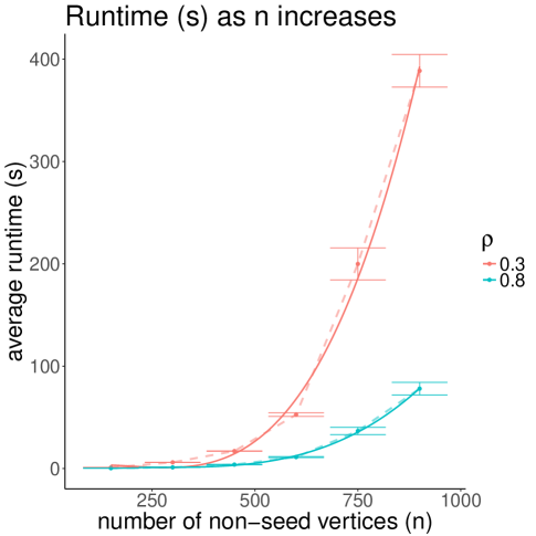
Figure 1: The average runtime (sec) plotted against the number of non-seed vertices $n$

The space demands of SGM are modest. Besides the obviously needed storage of $A$ and $B$ which, in general, requires $\Theta(n^{2})$ space, the Frank-Wolfe steps do not require any history beyond the current doubly stochastic matrix $\tilde{P}$ and its associated gradient (which is computed by matrix multiplication). The Hungarian Algorithm also requires just $O(n^{2})$ space, as does the subsequent one dimensional optimization (since there are three critical points to be tested, with a fixed number of matrix multiplications). Thus, the space requirements of SGM are just $O(n^{2})$, in total. (Note that even if the graphs are sparse, the gradients used in the Frank-Wolfe steps will not be sparse, in general, so that sparse implementations of the Hungarian Algorithm will not be helpful.)

2.4 Effectiveness of the SGM algorithm

Our main inference task is to recover an underlying, existing correspondence between the vertices of the two graphs —utilizing seeded graph matching, and we will soon focus on using the SGM algorithm for this purpose.

However, our first simulation experiment is instead narrowly focussed on the optimization task, which is to check if the SGM algorithm achieves the global optimum of the seeded graph matching problem that it approximates/tries to solve. As mentioned, there is no efficient algorithm for solving seeded graph matching, and SGM is an efficient algorithm, thus we have no hope of SGM consistently achieving the global optimum; indeed, in general, the most we can hope to obtain from SGM is a good approximate solution. However, we found that SGM does an excellent job of finding the global optimum for instances where we can compute the global optimum (with great effort!). Indeed, for small graphs we can compute the global optimum for seeded graph matching by expressing the problem as a linear integer programming problem, and then finding the exact solution using the discrete optimization solver GUROBI Optimizer [39]. We independently realized $50$ pairs of graphs $G_{1},G_{2}$ from a $.9$-SBM($3,b,\Lambda$) distribution with $\mathfrak{n}=30$ vertices, block assignment function $b$ such that each of the $k=3$ blocks has $10$ vertices, $m=2$ seeds discrete-uniformly randomly selected from the $30$ vertices, and

$$\Lambda=\begin{bmatrix}0.7&0.3&0.4\\ 0.3&0.7&0.3\\ 0.4&0.3&0.7\end{bmatrix}.$$ (9)

Running the SGM algorithm —as well as exactly solving seeded graph matching via GUROBI— on these $50$ pairs of graphs that we instantiated, we found that all $50$ were solved to global optimality by SGM. By contrast, when we repeated all of the above except without any seeds—in which case SGM is just FAQ—we found that only $23$ of the $50$ instantiations had FAQ achieving the global optimum.

Next, we return to the main inferential task, the estimation of an underlying correspondence. To demonstrate the effectiveness of the SGM algorithm, we independently realized $150$ pairs of graphs $G_{1},G_{2}$ for each value of $m=0,1,\ldots,20$ and each value of $\rho=0,0.1,0.2,\ldots,1$, on $\mathfrak{n}=n+m=300$ vertices from a $\rho$-SBM($k,b,\Lambda$) distribution, where $k=3$, $b$ is such that $\mathfrak{n}/3=100$ vertices belonged to each of the three blocks, and $\Lambda$ is as defined in Equation (9). The specific $m$ seeds used in each simulation were uniformly randomly selected from among the $\mathfrak{n}$ vertices.

For each pair of graphs, $G_{1},G_{2}$, we ran the SGM algorithm, and measured performance of the SGM algorithm in terms of the match ratio,

$$\delta:=\frac{|\{v\in V_{1}\backslash W_{1}:\phi(v)=\Psi(v)\}|}{n},$$ (10)

that is, the fraction of unseeded vertices of $G_{1}$ that are correctly matched. For any particular values of $m$ and $\rho$, let $\overline{\delta}$ denote the average match ratio taken over the 150 realizations.

For each $\rho=0,0.1,0.2,\ldots,1.0$, we plot in Figure 2 the average match ratio, $\overline{\delta}$, along with a confidence interval, as a function of the number of seeds, $m=0,1,\ldots,20$. (All confidence intervals used in this manuscript are of the form: mean $\pm$ twice the standard error, unless otherwise specified.) The expected number of vertices for which a discrete-uniformly randomly chosen bijection $V_{1}\rightarrow V_{2}$ agrees with $\Psi$ is $1$; thus, for a chance bijection, the mean of $\overline{\delta}$ would be $1/n=1/(\mathfrak{n}-m)$. As expected, $\overline{\delta}$ increases as $m$ increases and also as $\rho$ increases. Perfect performance when $\rho=1$ indicates that the SGM algorithm finds the isomorphism between graphs when it exists, while $\overline{\delta}\approx 1/n=$chance when $\rho=0$, since the natural alignment is then meaningless.

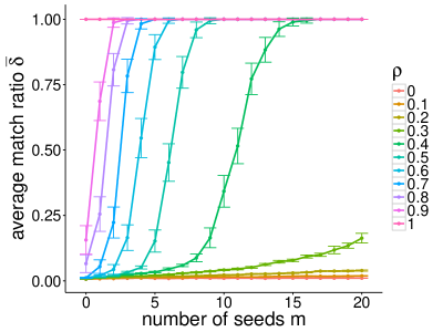
Figure 2: Average match ratio $\overline{\delta}\pm 2$s.e. as a function of the number of seeds $m$, for different correlation values $\rho$, in the $\rho$-SBM simulations of Section 2.4 on $\mathfrak{n}=300$ vertices.

2.5 Graph matching when the vertex sets are different sizes

Until this section, the vertex sets $V_{1}=\{1,2,\ldots,\mathfrak{n}\}$ and $V_{2}=\{1,2,\ldots,\mathfrak{n}\}$ have been assumed to be of the same cardinality as, indeed, there is assumed to be a natural correspondence between them in the form of a bijection $\Psi:V_{1}\rightarrow V_{2}$. For this section, suppose that $V_{1}=\{1,2,\ldots,\mathfrak{n}_{1}\}$ and $V_{2}=\{1,2,\ldots,\mathfrak{n}_{2}\}$ are such that $\mathfrak{n}_{1}<\mathfrak{n}_{2}$, and the underlying correspondence $\Psi:V_{1}\rightarrow V_{2}$ is merely injective (one-to-one), rather than bijective. We will use the expression “core vertices” for $V_{1}$ and its image through $\Psi$; the other $\mathfrak{n}_{2}-\mathfrak{n}_{1}$ vertices in $V_{2}$ will be called “extraneous vertices." As before, the seeds are taken as $W_{1},W_{2}=\{1,2,\ldots,m\}$ with the identity seeding function, for some $m<\mathfrak{n}_{1}$

The most straightforward way to treat this seeded graph matching setting is to pad $G_{1}$ in some fashion with additional vertices to bring the number of vertices associated with $G_{1}$ up to $\mathfrak{n}_{2}$, and then apply SGM as before. The vertices in $V_{2}$ matched to the padding are then identified as the extraneous vertices, and the remainder of the matching would approximate the natural correspondence $\Psi$ between $G_{1}$ and the matching subgraph of $G_{2}$. It would further seem that an innocuous choice of padding is to take the adjacency matrix $A$ for $G_{1}$ and append zeros to make the new adjacency matrix $A\oplus 0_{(\mathfrak{n}_{2}-\mathfrak{n}_{1})\times(\mathfrak{n}_{2}-\mathfrak{n}_{1})}$; this consists of adding $\mathfrak{n}_{2}-\mathfrak{n}_{1}$ isolated vertices to $G_{1}$.

Unfortunately, this choice is not innocuous. The effect of this padding scheme is to match $G_{1}$ to the best fitting subgraph of $G_{2}$, as opposed to the desired best fitting induced subgraph. Indeed, these isolated vertices of the padding will have an affinity to be matched to low-density subgraphs in $G_{2}$, even if these vertices in $G_{2}$ are core vertices. In this case, the correct correspondences for these $G_{2}$ vertices will not be correctly recovered by the matching. Indeed, in this manner the isolated vertices of the padding carry a lot of false signal—and are not merely the absence of signal that is desired to promote the (default) matching of the padded vertices in $G_{1}$ to the extraneous vertices of $G_{2}$.

Going back to the previous situation where $G_{1}$ and $G_{2}$ each have $\mathfrak{n}$ vertices and respective adjacency matrices $A,B$, define $\widetilde{A}:=2A-\vec{1}_{\mathfrak{n}}\vec{1}_{\mathfrak{n}}^{T}$ and $\widetilde{B}:=2B-\vec{1}_{\mathfrak{n}}\vec{1}_{\mathfrak{n}}^{T}$; these are effectively adjacency matrices, except that $1$ or $-1$ indicate adjacency or non-adjacency, respectively, instead of the usual $1$ or $0$. It is clear that substituting $\widetilde{A}$ and $\widetilde{B}$ in place of $A$ and $B$, respectively, in the seeded graph matching formulation of Equation (1) yields an equivalent optimization problem. It is then immediate that substituting $\widetilde{A}$ and $\widetilde{B}$ in place of $A$ and $B$, respectively, into the trace formulation of Equation (3) yields an equivalent optimization problem as well.

However, in our present setting where $G_{1}$ and $G_{2}$ respectively have $\mathfrak{n}_{1}$ and $\mathfrak{n}_{2}$ vertices and $\mathfrak{n}_{1}<\mathfrak{n}_{2}$, let us consider the effect of substituting $\widetilde{A}\oplus 0_{(\mathfrak{n}_{2}-\mathfrak{n}_{1})\times(\mathfrak{n}_{2}-\mathfrak{n}_{1})}$ and $\widetilde{B}$ in place of $A$ and $B$, respectively, in the seeded graph matching formulation in Equation (3). Indeed, for any particular permutation matrix $I_{m}\oplus P$ in that expression, consider the associated matching. The padded vertices in $G_{1}$ and the vertices which they are matched to in $G_{2}$ collectively add $0$ to the objective function, and the objective function is just $2$ times the difference between the number of edge agreements and the number of edge disagreements across the matching between the original vertices of $G_{1}$ and the vertices they are matched to in $G_{2}$. In summary, substituting $\widetilde{A}\oplus 0_{(\mathfrak{n}_{2}-\mathfrak{n}_{1})\times(\mathfrak{n}_{2}-\mathfrak{n}_{1})}$ and $\widetilde{B}$ in place of $A$ and $B$, respectively, in the seeded graph matching formulation in Equation (3) is equivalent to minimizing the number of edge disagreements under bijection $\phi$ from the vertices of $G_{1}$ to the vertices of an induced subgraph of $G_{2}$ with $\mathfrak{n}_{1}$ vertices, where the optimization variables are the possible $\mathfrak{n}_{1}$-vertex induced subgraphs of $G_{2}$ as well as the possible bijections between $G_{1}$ and the induced subgraph, also restricting that $\phi$ adheres to the seeding function for the seeds.

This formulation is ideal, in that the padding plays exactly the desired role. We therefore adopt this formulation for graph matching in the current setting where the number of vertices in $G_{1}$ and $G_{2}$ are different. The SGM algorithm applied to $\widetilde{A}\oplus 0_{(\mathfrak{n}_{2}-\mathfrak{n}_{1})\times(\mathfrak{n}_{2}-\mathfrak{n}_{1})}$ and $\widetilde{B}$ will be referred to as the adopted padding scheme, whereas applying SGM algorithm to $A\oplus 0_{(\mathfrak{n}_{2}-\mathfrak{n}_{1})\times(\mathfrak{n}_{2}-\mathfrak{n}_{1})}$ and $B$ will be referred to as the naïve padding scheme.

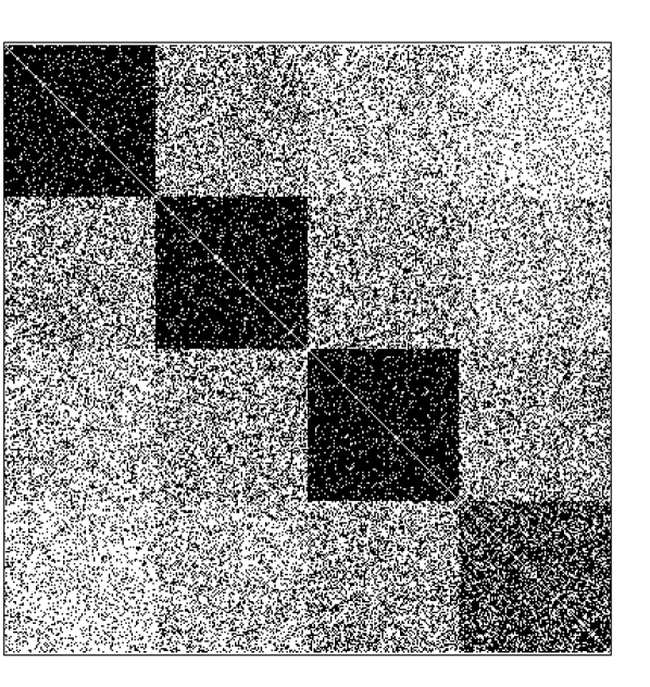
(a)

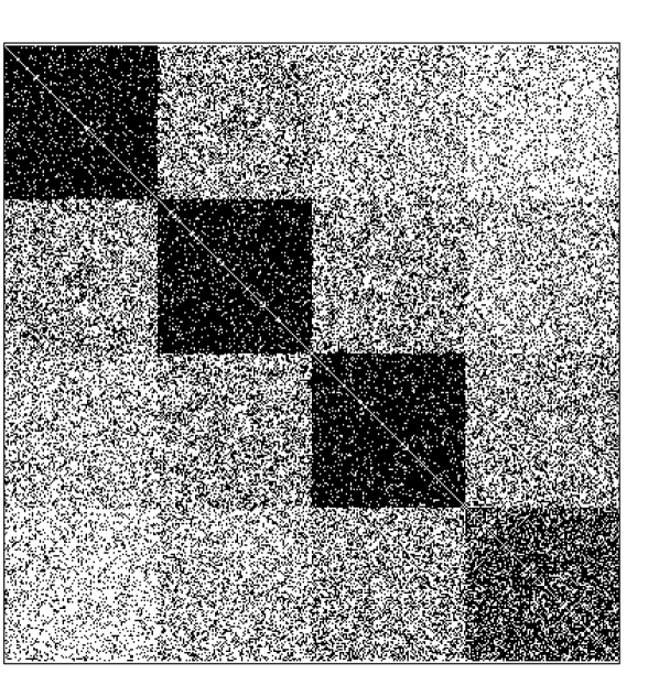
(b)

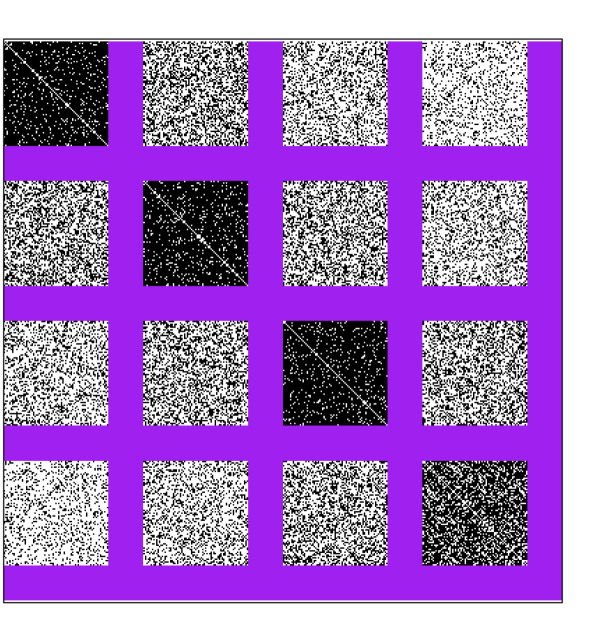
(c)

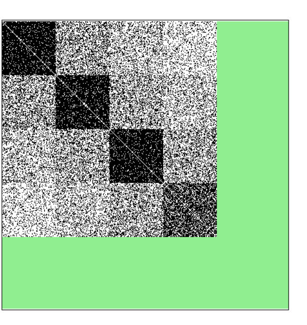
(d)

(e)

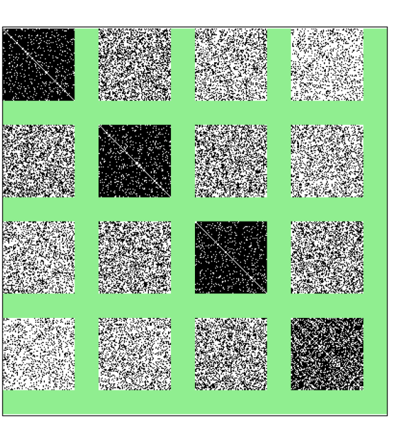
(f)

Figure 3: Section 2.5 illustration of naïve padding vs adopted padding:
a) Adjacency matrix for $G_{1}^{\prime}$; adjacency in black, nonadjacency in white. Four blocks of $100$ vertices each, $400$ vertices total, and the fourth block is less dense than the other three blocks.
b) Adjacency matrix for $G_{2}$; adjacency in black, nonadjacency in white. Four blocks of $100$ vertices each, $400$ vertices total, and the fourth block is less dense than the other three blocks.
c) Graph $G_{1}$ is obtained from $G_{1}^{\prime}$ by deleting $25$ vertices from each block (deleted vertices’ rows and columns in purple).
d) Adjacency matrix of $G_{1}$ (which has $300$ vertices) is (consolidated to) the upper left corner, then padding is added ($100$ green rows and columns at bottom and right).
e) Naïve padding; black, white, green in all these figures have respective values $1,0,0$. Pictured here is the adjacency matrix of padded-$G_{1}$, permuted by SGM to match $G_{2}$. Padded vertices were incorrectly paired to the fourth block in $G_{2}$, which has $75$ core vertices.
f) Adopted padding; black, white, green in all these figures have respective values $1,-1,0$. Pictured here is the adjacency matrix of padded-$G_{1}$, permuted by SGM to match $G_{2}$. SGM recovered the correct correspondences; padding was matched to the extraneous vertices.

To pictorially demonstrate the stark difference between these two padding schemes, we realized two graphs, $G_{1}^{\prime}$ and $G_{2}$, each having $400$ vertices, from a $0.5$-$SBM(4,b,\Lambda)$, where $b$ assigns $100$ vertices to each of the $k=4$ blocks, and

$$\Lambda=\begin{bmatrix}.9&.4&.3&.2\\ .4&.9&.4&.3\\ .3&.4&.9&.4\\ .2&.3&.4&.7\\ \end{bmatrix}.$$

Note that the fourth block is less dense than the other three blocks. The adjacency matrices of $G_{1}^{\prime}$ and $G_{2}$ are respectively pictured in Figures 3(a), 3(b). We obtained $G_{1}$ from $G_{1}^{\prime}$ by deleting $25$ uniformly randomly chosen vertices from each block of $G_{1}^{\prime}$; in Figure 3(c) the deleted vertices from $G_{1}^{\prime}$ are in purple. In Figure 3(d) the adjacency matrix of $G_{1}$ is in the upper left corner, and the padding is pictured in green. After selecting $10$ vertices uniformly at random from $G_{1}$ to be seeds, we applied the naïve padding scheme (wherein black, white, green in these figures have respective values $1,0,0$), as well as the adopted padding scheme (wherein black, white, green in these figures have respective values $1,-1,0$). In Figure 3(e), we see that the naïve padding scheme maps the padding of $G_{1}$ to the fourth block of $G_{2}$, even though $75$ of the vertices in the fourth block of $G_{2}$ are core vertices, not extraneous vertices. By contrast, in Figure 3(f) we see that the adopted padding scheme preserves the common community structure between $G_{1}$ and $G_{2}$, and the padding of $G_{1}$ is mapped to the extraneous vertices of $G_{2}$. Indeed, henceforth, we proceed to use the adopted padding scheme and call it Padded SGM; see Algorithm 2 for pseudocode.

  Input: Graphs $G_{1}$ and $G_{2}$ with respective vertex sets $\{1,\ldots,\mathfrak{n}_{1}\}$ and $\{1,\ldots,\mathfrak{n}_{2}\}$ and with respective adjacency matrices $A$ and $B$, assuming vertices $\{1,2,\ldots,m\}$ are seeds and assuming $\mathfrak{n}_{1}<\mathfrak{n}_{2}$

  Step 1: Compute $\tilde{A}:=2A-J_{\mathfrak{n}_{1}}$ and $\tilde{B}:=2B-J_{\mathfrak{n}_{2}}$;

  Step 2: Apply SGM Algorithm 1 to $\tilde{A}\oplus 0_{(\mathfrak{n}_{2}-\mathfrak{n}_{1})\times(\mathfrak{n}_{2}-\mathfrak{n}_{1})}$ and $\tilde{B}$ to obtain $\phi_{\hat{P}}$;

  return $\hat{\phi}_{r}$, the restriction of $\phi_{\hat{P}}$ to the vertices of $G_{1}$.

Algorithm 2 Padded SGM

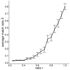
Figure 4: The average match ratio $\overline{\delta}$ plotted against the ratio $r=|V_{1}|/|V_{2}|=\mathfrak{n}_{1}/300$ for the simulation experiment in Section 2.5.

We next proceed to utilize Algorithm 2 Padded SGM when matching graphs on differently sized vertex sets. For each value of $r=0.25,0.30,\ldots,1$, we realized $300$ pairs of graphs $G_{1}^{\prime}$ and $G_{2}$ from a $0.7$-SBM($3,b,\Lambda$), where there are $300$ vertices evenly divided among the three blocks and where $\Lambda$ is given in Equation (9). $G_{1}$ is created by deleting vertices in $G_{1}^{\prime}$ in such a way that $G_{1}$ has $r\cdot 300$ vertices and an equal number of vertices in each block. In Figure 4, we apply Algorithm 2 to $G_{1}$ and $G_{2}$ using a randomly selected seed set of size $m=3$, and plot the mean (with confidence interval) of the average match ratio $\overline{\delta}$ against the ratio $r=\mathfrak{n}_{1}/\mathfrak{n}_{2}$. We note that in the small $r$ settings, Padded SGM poorly recovers the true correspondence between the smaller graph and the core of the larger network.

While this seems an indictment on our padding approach, we have observed that the matching obtained via Algorithm 2 can be better in terms of the objective function being evaluated than the true permutation in low $r$ settings. In these cases, graph matching methods are not suited for finding the true correspondence. Understanding this phenomena further is the subject of future research.

2.6 SoftSGM

As mentioned, seeded graph matching is an intractable problem. Thus, because the SGM algorithm is an efficient algorithm, SGM will not in general find the global optimal solution; indeed, the realistic goal of SGM is to find a local optimum that is not too far from the global optimal solution. Ironically, this shortcoming has a very profitable silver lining, as we next explain.

Even if we could compute the global optimal solution for seeded graph matching, there is still a not-insignificant chance that the global optimal solution is not equal to the natural correspondence function $\Psi$. In light of this, it may be quite helpful for a practitioner to have available several other near-optimal seeded graph matchings that would provide alternative possibilities, just in case the practitioner happens to learn through other means that the global optimal match—or a single highly-touted local optimal match—for a particular vertex is actually mistaken. It would be even more valuable to be able to create, for each vertex in one of the graphs, a ranked list of the vertices in the other graph, ranked by a confidence of being a match. This can be achieved through sampling local optima near the seeded graph matching global optimum, and then creating rankings based on the fraction of time in the sample that pairs of vertices are matched via a local optimum in the sample.

  Input: Graphs $G_{1},G_{2}$ each with vertex set $\{1,2,\ldots,m+n\}$, assuming vertices $\{1,2,\ldots,m\}$ are seeds$R\in\mathbb{N};$ number of restarts of SGM algorithm,$\gamma\in[0,1];$ random initialization step size

  for $i=1:R$ do

     Step 1: Select $Q_{i}$ uniformly at random from the set of $n\times n$ permutation matrices;

     Step 2: Realize $\beta_{i}$ from a Uniform($0,\gamma$);

     Step 3: $P^{(0)}_{i}:=\beta_{i}Q_{i}+(1-\beta_{i})\frac{1}{n}\vec{1}_{n}\vec{1}_{n}^{T};$

     Step 4: Apply SGM Algorithm 1 to $G_{1},G_{2}$ initialized at $P^{(0)}_{i}$ to obtain $\phi_{\hat{P}}$

     Step 5: Set $P_{i}:=\hat{P}$;

  end for

  Step 6: Set $T:=I_{m}\oplus\left(\frac{1}{R}\sum_{i=1}^{R}P_{i}\right)$.

  return $T$

Algorithm 3 SoftSGM

Specifically, in our setting of Section 1.1, given graphs $G_{1}$ and $G_{2}$ each with vertex set $V=\{1,2,\ldots,\mathfrak{n}\}$, the Soft Match SGM Algorithm (or SoftSGM) consists of running SGM repeatedly on $G_{1}$,$G_{2}$ from randomly sampled starting doubly stochastic matrices $P^{(0)}\in{\mathcal{D}}_{n}$ (where $n$ is the number of non-seeds), with $R$ denoting the number of such “restarts." Indeed, precisely because SGM will not, in general, solve the seeded graph matching problem to global optimality, we will typically obtain a sample of seeded graph matching approximate solutions, many of which being different from each other. For each $i,j\in V$, we will define $T_{ij}$ to be the number of sample instances in which vertex $i$ in $G_{1}$ was matched to vertex $j$ in $G_{2}$, divided by ($R$) the total number of sample instances; this fraction will serve as a confidence for the pair $i,j$ being a match, and these values create, for each vertex in $G_{1}$, a probability distribution over possible matches. For each vertex in $G_{1}$, ordering the vertices of $G_{2}$ by decreasing match probability then creates a ranked list of possible matches to the vertices of $G_{2}$. See Algorithm 3 for pseudocode of the SoftSGM algorithm.

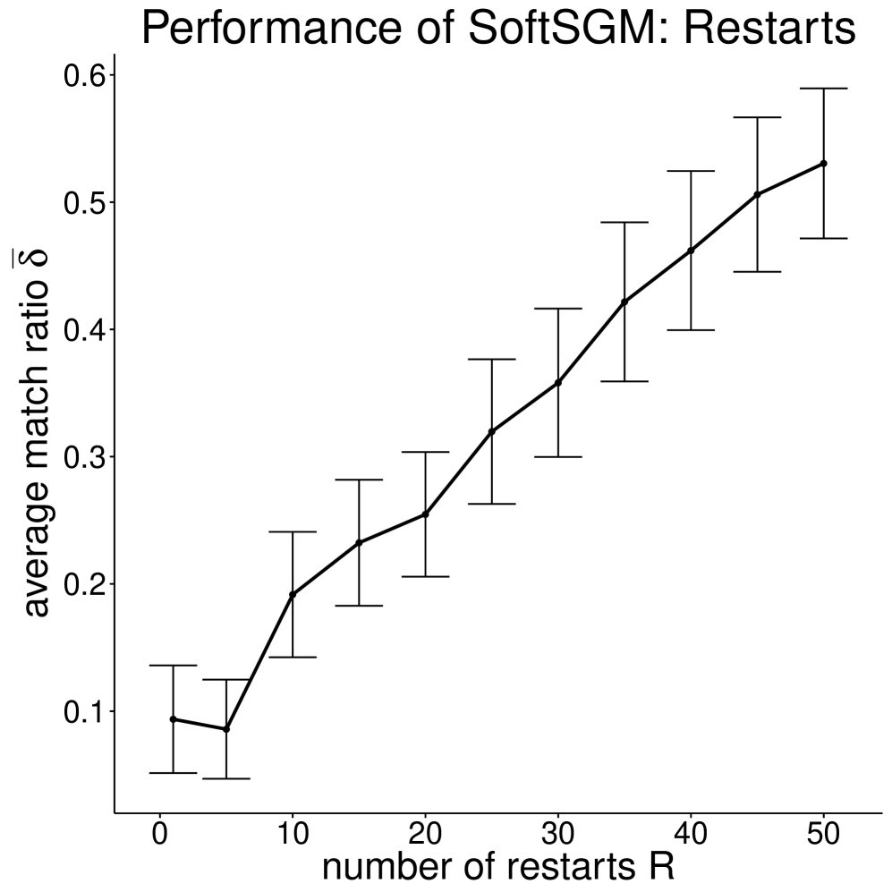
(a) $m=3$ seeds, depth $K=1$, correlation $\rho=0.6$, varying number of restarts $R$

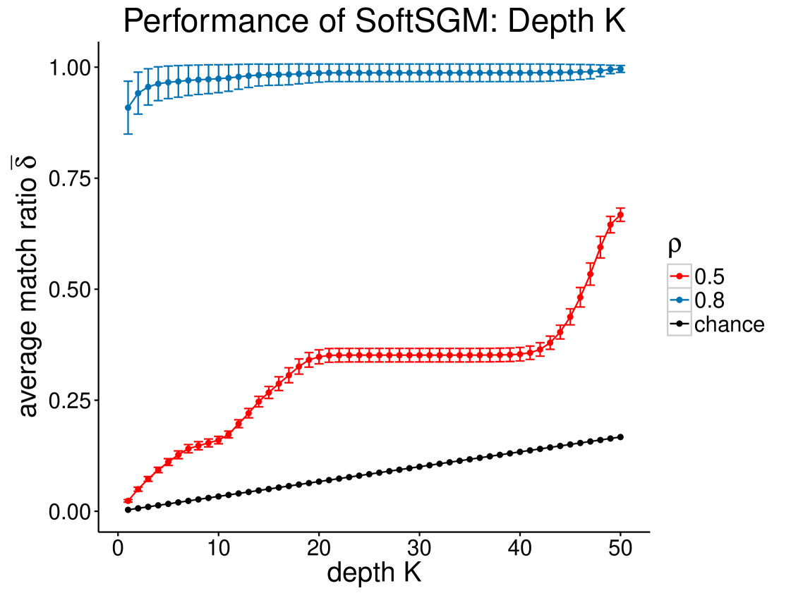
(b) $m=0$ seeds, number of restarts $R=50$, varying depth $K$, correlation $\rho=0.5$ (red), $\rho=0.8$ (blue)

Figure 5: SoftSGM simulations; effects of number of restarts $R$ and depth $K$ on average match ratio $\overline{\delta}$.

As a first experiment, we independently realized $50$ pairs of graphs $G_{1}$,$G_{2}$ from a $.7$-SBM($3,b,\Lambda$) distribution with $\mathfrak{n}=30$ vertices, block assignment function $b$ such that each of the $k=3$ blocks has $10$ vertices, $m=4$ seeds discrete-uniformly randomly selected from the $30$ vertices, and $\Lambda$ as defined in Equation (9). As mentioned before, for such small graphs we can compute the global optimum for seeded graph matching by expressing it as a linear integer programming problem, and then solving it exactly with the very powerful software package GUROBI Optimizer. Among all of the $50\cdot 30=1500$ vertices involved, all but two were matched (through global optimum from GUROBI) to their correct corresponding vertex. However, even the two remaining vertices that were not correctly matched had their corresponding vertex appear in second place in their respective ranked lists provided by SoftSGM with $R=50$ restarts. In summary, even optimal graph matching might not match a vertex to its corresponding vertex, and it is useful for a practitioner to have the ranked list provided by SoftSGM as a recourse. In the next experiments, the sizes of the graphs are larger, and computing the global minimum seeded graph match solution is not remotely practical.

Since SoftSGM provides each vertex with a ranked list of possible matches (rather than a single proposed matched vertex), we need to tweak the definition of “match ratio” when we want to measure the effectiveness of SoftSGM. Let $K\in\mathbb{N}$ be fixed; $K$ will be called the match ratio depth. In a single SoftSGM simulation, each vertex $i$ in $G_{1}$ is called successfully matched at depth $K$ if its corresponding vertex $\Psi(i)$ is one of the top $K$ vertices in the ranked list associated with $i$. The match ratio $\delta$ for the simulation is defined to be the fraction of the non-seed vertices of $G_{1}$ which are successfully matched at depth $K$. If multiple simulations are done, then the average match ratio $\overline{\delta}$ is defined to be the average of the match ratios over all of the simulations.

To demonstrate how the number of restarts, $R$, impacts the SoftSGM algorithm, for each $R=1,5,10,\ldots,50$, we independently realize $100$ pairs of graphs from $0.6$-SBM($3,b,\Lambda$) where there are $\mathfrak{n}=300$ vertices divided evenly into $3$ blocks, with $\Lambda$ given in Equation (9). We then apply Algorithm 3, SoftSGM, to each pair of graphs using $m=3$ uniformly randomly selected seeds, and using depth $K=1$. We plot the average match ratio $\overline{\delta}$ against the number of restarts $R$ in Figure 5(a). Note that increasing $R$ yields dramatic improvement. Of course, when $R=1$ the SoftSGM algorithm is just implementing Algorithm 1, since $K=1$ here.

Next, for correlation values $\rho=0.5$ and $\rho=0.8$ we apply the SoftSGM algorithm with $R=50$ restarts and no seeds to $50$ pairs of graphs independently realized from $\rho-SBM(3,b,\Lambda)$ where the $\mathfrak{n}=300$ vertices are evenly divided into $3$ blocks and $\Lambda$ is as given in Equation (9). In Figure 5(b) we plot, for each of $\rho=0.5$ (red curve) and $\rho=0.8$ (blue curve), the average match ratio $\overline{\delta}$ as a function of the depth $K$. This experiment points to the utility of SoftSGM in the limited seeding regime: while SGM alone may not recover the true correspondences, SoftSGM can greatly increase precision at even modest depth, allowing practitioners the chance to identify the correct correspondences without having to search the entire vertex set.

3 Real-Data Demonstrations

Thus far we have seen the applicability of the SGM algorithm in simulated examples involving graphs realized from a $\rho$-correlated stochastic block model. We now illustrate performance of the SGM algorithm on three real-data network pairs.

3.1 Wikipedia

Wikipedia is an online editable encyclopedia with (as of April 2017) 40 million articles (more than 5.3 million articles in English) in 293 languages. A collection of $\mathfrak{n}=1382$ English articles were collected by crawling the (directed) 2-neighborhood of the document “Algebraic Geometry” using hyperlinks to traverse from one English article to another. The vertices in this network are the webpages, with an edge adjoining one vertex to the next if the first webpage contains a hyperlink to the second. This first graph was made into a simple undirected graph by symmetrizing its adjacency matrix. In Wikipedia, inter-language links between articles of the same topic in different languages are available; thus, there is a one-to-one correspondence between the vertices of this English Wikipedia subgraph and associated vertices of the French Wikipedia graph. Corresponding articles in French were collected and their intra-language hyperlink structure yielded a second graph (not necessarily connected) which was also symmetrized. The English Wikipedia subgraph is denoted $G_{2}$ and the French Wikipedia subgraph induced by the correspondents of the English Wikipedia articles is denoted $G_{1}$; thus $G_{1}$ and $G_{2}$ both have 1382 vertices representing webpages, and each webpage in the English graph has a naturally corresponding webpage in the French graph.

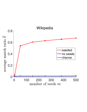
Figure 6: Average match ratio $\overline{\delta}$ as a function of number of seeds $m$ for the the Wikipedia graph; SGM is red, SGM with no seeds (seeds deleted) is blue, chance is black.

We perform $100$ independent replicates of the following. For each value of $m=0,5,50,150,250,382,500$, we discrete-uniformly randomly select $m$ seeds and use these seeds for seeded graph matching of the French and English Wikipedia subgraphs $G_{1}$ and $G_{2}$ using the SGM algorithm. Figure 6 depicts, in red, the average match ratio $\overline{\delta}$ (along with one standard error) as a function of the number of seeds $m$ and, in black, the expected average match ratio of chance (i.e. if vertices were paired uniformly at random), which is $1/(1382-m)$. We see dramatic performance improvement from incorporating just a few seeds: with no seeds $\overline{\delta}\approx 1/100$ (chance is $1/1382$), while with just $m=50$ seeds $\overline{\delta}>1/2$ (chance is $1/1332$). The blue curve in Figure 6 shows the average match ratio $\overline{\delta}$ for the unseeded problem on $\mathfrak{n}-m$ vertices (i.e. with the selected $m$ seeds removed from the two graphs and then applying SGM with no seeds). While the problem becomes smaller as $m$ increases, performance does not improve appreciably. Of note, when using $m=50$ seeds and using the Padded SGM algorithm to match the English network with the largest connected component of the French network (which has 1323 vertices), the match ratio was approximately 0.203.

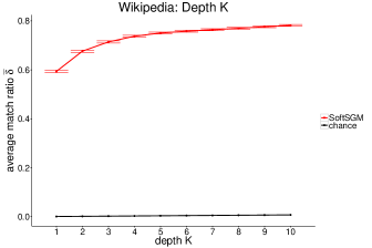
Figure 7: SoftSGM applied to French and English Wikipedia graphs. Average match ratio $\overline{\delta}$ at depth $K$ plotted using $m=40$ seeds and $R=25$ restarts. Chance is plotted in black.

The next experiment consists of discrete-uniformly randomly selecting $m=40$ seeds in $G_{1},G_{2}$ and applying Algorithm 3: SoftSGM using $R=25$ restarts. We did $25$ independent realizations of this experiment, and Figure 7 shows the average match ratio vs depth $K$ for $K=1,2,\ldots,10$. Note the improvement brought about by having the ranked list rather than just a single match for each vertex. In Figure 7, plotted in black is $K/(1382-40)$ for each value of $K$, which is the expected average match ratio of chance at depth $K$ (i.e. if the vertices were ordered by uniformly random permutation).

3.2 Enron

As reported in [40], “Enron Corporation was an American energy, commodities, and services company. Before its bankruptcy on December 2, 2001, Enron was one of the world’s major electricity, natural gas, communications, and pulp and paper companies, with claimed revenues of nearly $101 billion during 2000. Fortune named Enron America’s Most Innovative Company for six consecutive years. At the end of 2001, it was revealed that its reported financial condition was sustained by institutionalized, systematic, and creatively planned accounting fraud, known since as the Enron scandal. Enron has since become a well-known example of willful corporate fraud and corruption. The scandal also brought into question the accounting practices and activities of many corporations in the United States and was a factor in the enactment of the Sarbanes-Oxley Act of 2002. The scandal also affected the greater business world by causing the dissolution of the Arthur Andersen accounting firm.”

In the wake of the Enron Scandal, the Justice Department released a vast collection of email messages which have been posted online for academic use; since privacy constraints usually keep large collections of email out of reach, this data set is both unique and valuable to the research community [41]. The Enron email corpus consists of messages amongst $\mathfrak{n}=184$ employees of the Enron Corporation. Publicly available emails are used to compute a time series of graphs $\{G_{t}:t=1,\ldots,T\}$ where each graph represents one week of emails in which a node represents an email address and an edge represents an email sent between the two addresses during the given week. An important inference task is to identify “chatter” anomalies — small groups of actors whose activity amongst themselves increases significantly for some week $t$ — since this could potentially indicate conspiratorial activity amongst the actors. Previous work has identified such an anomaly at week $t=132$ (see [42]).

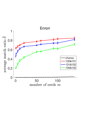
Figure 8: For each pair of graphs from $\{G_{t}:t=130,131,132\}$, the average match ratio $\overline{\delta}$ is plotted against the number of seeds $m$.

The Enron email graphs for consecutive weeks $t=130,131,132$ are matched, one pair at a time, using SGM, for each of $100$ randomly chosen seed sets of size $m$, for each of $m=0,1,5,10,20,50,60,$ $90,100,140$. Figure 8 plots, for each pair of graphs, the average match ratio, $\overline{\delta}$, along with one standard error, against the number of seeds $m$. (Chance is plotted in black.) The results are consistent with the finding reported in [42]; indeed, the average match ratio $\overline{\delta}$ is much higher between the graphs for weeks $t=130,131$, where there was no significant change, compared to matching across the change between the graphs for weeks $t=131,132$ and between the graphs for weeks $t=130,132$. Investigation shows that the difference in performance is largely attributable to the vertices participating in the anomaly, as reported in [42].

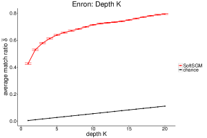
Figure 9: SoftSGM applied to $G_{130}$ and $G_{132}$. Average match ratio $\overline{\delta}$ at depth $K$ plotted using $m=5$ seeds and $R=50$ restarts. Chance is plotted in black.

Next, we do $250$ independent replicates of the following experiment. SoftSGM is performed on $G_{130},G_{132}$ with $m=5$ discrete-uniformly randomly chosen seeds and $R=50$ restarts. Figure 9 plots the average match ratio $\overline{\delta}$ against depth $K=1,2,\ldots,20$. Note that SGM — without restarts — had average match ratio $\overline{\delta}\approx 0.65$ when using $m=140$ seeds, but with $R=50$ restarts and depth $K=20$ the average match ratio is $\overline{\delta}\approx 0.80$ with only $m=5$ seeds.

3.3 C. elegans

C. elegans is a roundworm that has been extensively studied (see for example [43, 44, 45, 46]). We consider $\mathfrak{n}=279$ neurons in its simple nervous system, and the connections have been fully mapped in [46]; this mapping was a very important milestone in connectomics. There are two types of connections between neurons: chemical synapses and electrical synapses. We denote by $G_{1}$ and $G_{2}$ the graphs for which vertices represent neurons and edges represent electrical synapses and chemical synapses, respectively. While these graphs are often weighted and directed, for simplicity and uniformity with our other examples we take $G_{1}$ and $G_{2}$ as unweighted and undirected.

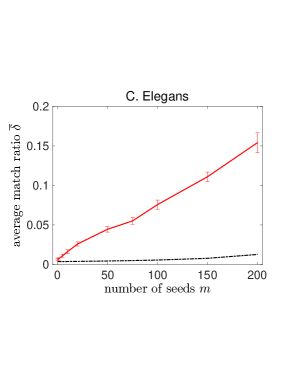
Figure 10: The average match ratio $\overline{\delta}$ plotted (in red) against number of seeds $m$ when matching the Electrical and Chemical connectivity graphs of C. elegans nervous system. (Chance is in black.)

For each $m=0,1,5,10,20,50,75,100,150,200$, we discrete-uniformly randomly select $100$ sets of $m$ seeds from the vertex set and, for each set of seeds in turn, we apply Algorithm 1: SGM to the C. elegans connectivity graphs. In Figure 10 we plot the average match ratio $\overline{\delta}$ and one standard error (red) against the number of seeds $m$. (Chance is plotted in black.) Using Padded SGM to match the chemical synapse network with the largest connected component of the electrical synapse network (which has $248$ vertices), the match ratio was approximately $0.028$ using $m=50$ seeds.

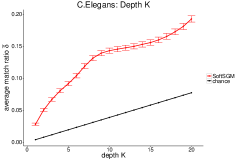
(a) Using Algorithm 3: SoftSGM with $m=20$ seeds and $R=50$ restarts for increasing $K$.

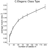
(b) Matching classes (inter-, motor, and sensory neuron) using Algorithm 1: SGM with $m$ seeds.

Figure 11: Matching the chemical and electrical networks of the C. elegans worm and plotting performance in terms of the average match ratio $\overline{\delta}$.

Next, we do $150$ independent replicates of the following experiment. Algorithm 3: SoftSGM is used to match the chemical and electrical networks using $m=20$ seeds and $R=50$ restarts. Figure 11(a) plots the average match ratio $\overline{\delta}$ against depth $K=1,2,\ldots,20$. While only approximately $16\%$ of the vertices can be correctly matched across the two networks even when using $m=200$ seeds (that is, more than $2/3$ of the correspondences are already known), nearly $20\%$ of the vertices can be correctly matched at depth $K=20$ when using only $m=20$ seeds.

Each of the neurons in C. elegans is classified as being either a motor neuron, interneuron, or a sensory neuron. For our next experiment we explore what proportion of the C. elegans vertices/neurons are matched by SGM to a vertex/neuron from the same class (ie., a motor neuron to a motor neuron, etc.). For each $m=0,1,5,10,25,50,75,100,150,200$, we discrete-uniformly randomly generate $100$ sets of $m$ seeds and, for each of these seed sets, we apply SGM to $G_{1}$, $G_{2}$. In this context, we consider a vertex to be correctly matched if it is matched to a vertex with the same class, and average match ratio $\overline{\delta}$ is define accordingly. In Figure 11(b) we plot $\overline{\delta}$ as a function of the number of seeds. While SGM performs relatively poorly in recovering the exact correspondence between neurons, it performs significantly better in recovering neural classes across networks. This suggests that the correlation across networks is not at the vertex level, rather at the neuronal class level, with neurons of the same type behaving similarly across network modalities.

4 Comparing SGM to seeded PATH on QAPLIB

As mentioned in Section 1, the PATH Algorithm [32] is a popular graph matching algorithm that is used in practice. The algorithm consists of considering a sequence of formulations of the underlying problem, starting with a convex formulation, and ending at a concave formulation, and the sequence of intermediate formulations traverse a “path” along the convex combination of the initial and final formulation. Approximate solutions to one formulation serve as the starting point for the next formulation, and Frank-Wolfe methodology is used on each formulation.

We converted the PATH algorithm to a seeded version, which we call sPATH, by fixing the alignment variables that correspond to the seeds so that they always reflect the seed correspondences, and the fixed values of these variables are then propagated through the algorithm.

In this section we compare SGM to sPATH on test problems from QAPLIB, a library of $137$ quadratic assignment problem instances [31]. Sixteen of these benchmark quadratic assignment problem instances were deemed particularly challenging, and were therefore used in [23], [32], [29] to compare the performance of graph matching algorithms. For fifteen of the sixteen we were able to access the optimal permutation, and not just the optimal objective function value; of course, for seeding we want this optimal permutation. Note that the quadratic assignment problem is precisely the optimization problem in Eq. (3), except that the maximization is, instead, minimization, and the matrices $A$ and $B$ are not necessarily adjacency matrices, but can have any real values as entries. The orders of the matrices in these fifteen problem instances range from $12$ to $40$. Of course, modifying the algorithms from maximization to minimization is trivially accomplished by appropriate negations.

For each of the fifteen benchmark quadratic assignment problem instances, and for each value of $m=1,2,3,4$, we did $30$ independent experiments of randomly selecting $m$ seeds, and we compared the average (over the thirty experiments) objective function values of SGM to sPATH and to the optimal solution, see Table 1 for these results. On these benchmarks, SGM was more effective than sPATH.

The PATH algorithm code we accessed [32] was written in C++, and we seeded it directly in its native C++, writing the adjustments into the original code, whereas our SGM algorithm is written in R. (Also, while SGM was run on a laptop with Intel Core i5 @ 1.6 GHz, sPATH was run on the MARCC computer with specs as given in subsection 2.3.) The average runtimes for the experiments on the larger benchmarks were on the order of $0.01$ seconds for SGM and $0.14$ seconds for PATH. Because the runtimes for sPATH are an order of magnitude greater than for SGM (and are indeed so, more generally), sPATH is not comparable more broadly to SGM, and we therefore do not include more comparison.

QAP	OPT	$m=1$		$m=2$		$m=3$		$m=4$
		SGM	sPATH	SGM	sPATH	SGM	sPATH	SGM	sPATH
chr12c	11156	18770	31858	16298	30889	16221	27031	14504	25073
chr15a	9896	15813	49522	16280	42959	15861	35591	14399	32041
chr15c	9504	18230	45144	15649	40329	15494	36909	14027	35654
chr20b	2298	3555	9411	3585	8991	3540	8091	3556	7521
chr22b	6194	8359	14075	8184	13503	8021	13126	7673	12475
esc16b	292	293	308	295	304	294	301	293	301
rou12	235528	250799	285085	242999	276292	236993	268722	236432	264059
rou15	354210	369198	449821	361721	439908	357969	415076	356537	402067
rou20	725522	748128	863811	753645	886876	746137	855938	743474	850498
tai15a	388214	403314	463836	402760	461114	398765	449411	396544	438072
tai17a	491812	518678	590697	506259	596524	506159	575686	502410	563565
tai20a	703482	736797	855532	739771	852671	735472	850778	716565	828659
tai30a	1818146	1888526	2141265	1878886	2123362	1874521	2119654	1865151	2109946
tai35a	2422002	2515301	2876351	2505556	2838981	2504548	2812018	2493860	2800284
tai40a	3139370	3255807	3716363	3261394	3662562	3246184	3630483	3249476	3611428

Table 1: Average objective function from minimization via SGM and sPATH (as well as the optimal solution) on 15 benchmark examples of the QAPLIB library, with $m=1,2,3,4$ seeds.

5 Discussion

Many graph inference tasks involve multiple graphs consisting of corresponding vertex sets. These tasks are more easily accomplished if we know the correspondence between the vertices in the different graphs, but these correspondences might be hidden from us. Data fusion based on such a correspondence, if it can be (at least approximately) recovered, will result in data representation that reveals hidden relationships between graph vertices, providing a more complete worldview.

In this manuscript we modify the (theoretically principled and computationally tractable) graph matching FAQ algorithm of Vogelstein et al (2015) [23] to obtain what we call the SGM algorithm and its variants, which

1. Incorporate the use of seeds,

2. Can match graphs of different orders (i.e., are differently sized), and

3. Can provide a soft matching which assigns —to each pair of vertices across the two graphs— a value representing our confidence that the pair correspond.

We demonstrated the effectiveness of the SGM algorithm and its variants via simulations and three real data experiments. In particular, seeding can provide a dramatic increase in the success of recovering underlying vertex correspondence. Also, soft matching provides each vertex with a ranked list of potential correspondents instead of a single proposed correspondent, which leaves the practitioner with recourse in the event of discovery (by other means) that a proposed correspondent is not correct.

In practice, identifying seeds may be costly. Thus, it will be important to understand the cost-benefit trade-off between inference without correspondence vs inference performed subsequent to seed discovery and utilization. This paper provides the foundation for that analysis. Note that the value of a few seeds leads to the demand for an active learning methodology to identify the most cost-effective vertices to use as seeds, for example see [20].

Obvious extensions to this work include: (a) the case where the correspondence may be many-to-many; and (b) the case where the seeds themselves are soft/errorful; this means that we know that it is likely (but not certain) that various pairs of vertices correspond. Each of these extensions can be addressed within the framework presented here.

Also, there are more general notions of closeness between graphs, such as graph edit distance. See [47] for analysis and a successful algorithmic approach for this form of graph matching. It would be profitable to consider ways to seed this algorithm.

In conclusion, we contend that the methodology presented herein forms the foundation for improving performance in myriad graph inference applications for which there exists a partially known-or-discoverable correspondence between the vertices of various graphs.

References

- [1] Y. Lu, K. Huang, and C.-L. Liu, “A fast projected fixed-point algorithm for large graph matching,” Pattern Recognition, vol. 60, pp. 971–982, 2016.
- [2] K. Riesen and M. Ferrer, “Predicting the correctness of node assignments in bipartite graph matching,” Pattern Recognition Letters, vol. 69, pp. 8–14, 2016.
- [3] J. Lerouge, Z. Abu-Aisheh, R. Raveaux, P. Héroux, and S. Adam, “New binary linear programming formulation to compute the graph edit distance,” Pattern Recognition, vol. 72, pp. 254–265, 2017.
- [4] J. Sang and C. Xu, “Robust face-name graph matching for movie character identification,” IEEE Transactions on Multimedia, vol. 14, no. 3, pp. 586–596, 2012.
- [5] A. Egozi, Y. Keller, and H. Guterman, “A probabilistic approach to spectral graph matching,” IEEE Transactions on Pattern Analysis and Machine Intelligence, vol. 35, no. 1, pp. 18–27, 2013.
- [6] S. Iodice and A. Petrosino, “Salient feature based graph matching for person re-identification,” Pattern Recognition, vol. 48, no. 4, pp. 1074–1085, 2015.
- [7] P. Pedarsani and M. Grossglauser, “On the privacy of anonymized networks,” in Proceedings of the 17th ACM SIGKDD international conference on Knowledge discovery and data mining, pp. 1235–1243, ACM, 2011.
- [8] L. Yartseva and M. Grossglauser, “On the performance of percolation graph matching,” in Proceedings of the first ACM conference on Online social networks, pp. 119–130, ACM, 2013.
- [9] L. Chen, J. T. Vogelstein, V. Lyzinski, and C. E. Priebe, “A joint graph inference case study: The C.Elegans chemical and electrical connectomes,” in Worm, vol. 5, p. e1142041, Taylor & Francis, 2016.
- [10] F. Yang and F. Kruggel, “A graph matching approach for labeling brain sulci using location, orientation, and shape,” Neurocomputing, vol. 73, no. 1-3, pp. 179–190, 2009.
- [11] D. Conte, P. Foggia, C. Sansone, and M. Vento, “Thirty years of graph matching in pattern recognition,” International Journal of Pattern Recognition and Artificial Intelligence, vol. 18, no. 3, pp. 265–298, 2004.
- [12] P. Foggia, G. Perncannella, and M. Vento, “Graph matching and learning in pattern recognition in the last 10 years,” Internation Journal of Pattern Recognition and Artificial Intelligence, vol. 28, no. 1, 2014.
- [13] J. Yan, X.-C. Yin, W. Lin, C. Deng, H. Zha, and X. Yang, “A short survey of recent advances in graph matching,” in Proceedings of the 2016 ACM on International Conference on Multimedia Retrieval, pp. 167–174, ACM, 2016.
- [14] S. Sahni and T. Gonzalez, “P-complete approximation problems,” Journal of the ACM (JACM), vol. 23, no. 3, pp. 555–565, 1976.
- [15] L. Babai, “Graph isomorphism in quasipolynomial time,” arXiv preprint arXiv:1512.03547, 2016.
- [16] M. Zaslavskiy, F. Bach, and J.-P. Vert, “Global alignment of protein–protein interaction networks by graph matching methods,” Bioinformatics, vol. 25, no. 12, pp. 1259–1267, 2009.
- [17] C. Fraikin and P. Van Dooren, “Graph matching with type constraints on nodes and edges,” in Dagstuhl Seminar Proceedings, (Dagstuhl, Germany), Schloss Dagstuhl-Leibniz-Zentrum für Informatik, 2007.
- [18] J. Ham, D. D. Lee, and L. K. Saul, “Semisupervised alignment of manifolds.,” in AISTATS, pp. 120–127, 2005.
- [19] V. Lyzinski, D. L. Sussman, D. E. Fishkind, H. Pao, L. Chen, J. T. Vogelstein, Y. Park, and C. E. Priebe, “Spectral clustering for divide-and-conquer graph matching,” Parallel Computing, vol. 47, pp. 70–87, 2015.
- [20] L. Li and W. M. Campbell, “Matching community structure across online social networks,” Network NIPS, 2015.
- [21] N. Hu, R. M. Rustamov, and L. Guibas, “Graph matching with anchor nodes: A learning approach,” pp. 2906–2913, 2013.
- [22] E. Kazemi, S. H. Hamed, and M. Grossglauser, “Growing a graph matching from a handful of seeds,” Proceedings of the VLDB Endowment, vol. 8, no. 10, pp. 1010–1021, 2015.
- [23] J. T. Vogelstein, J. M. Conroy, V. Lyzinski, L. J. Podrazik, S. G. Kratzer, E. T. Harley, D. E. Fishkind, R. J. Vogelstein, and C. E. Priebe, “Fast approximate quadratic programming for graph matching,” PLOS one, vol. 10, no. 4, p. e0121002, 2015.
- [24] V. Lyzinski, S. Adali, J. T. Vogelstein, Y. Park, and C. E. Priebe, “Seeded graph matching via joint optimization of fidelity and commensurability,” arXiv preprint arxiv:1401.3813, 2014.
- [25] V. Lyzinski, D. Fishkind, and C. Priebe, “Seeded graph matching for correlated Erdős-Rènyi graphs,” Journal of Machine Learning Research, vol. 15, pp. 3693–3720, 2014.
- [26] V. Lyzinski, D. L. Sussman, M. Tang, A. Athreya, and C. E. Priebe, “Perfect clustering for stochastic blockmodel graphs via adjacency spectral embedding,” Electronic Journal of Statistics, vol. 8, no. 2, pp. 2905–2922, 2014.
- [27] D. E. Fishkind, V. Lyzinski, H. Pao, L. Chen, and C. E. Priebe, “Vertex nomination schemes for membership prediction,” The Annals of Applied Statistics, vol. 9, no. 3, pp. 1510–1532, 2015.
- [28] V. Lyzinski, “Information recovery in shuffled graphs via graph matching,” arXiv preprint arXiv:1605.02315, 2016.
- [29] V. Lyzinski, D. E. Fishkind, M. Fiori, J. T. Vogelstein, C. E. Priebe, and G. Sapiro, “Graph matching: Relax at your own risk,” IEEE Transactions on Pattern Analysis and Machine Intelligence, vol. 38, pp. 60–73, Jan 2016.
- [30] V. Lyzinski, K. Levin, D. E. Fishkind, and C. E. Priebe, “On the consistency of the likelihood maximization vertex nomination scheme: Bridging the gap between maximum likelihood estimation and graph matching,” Journal of Machine Learning Research, vol. 17, no. 179, pp. 1–34, 2016.
- [31] R. E. Burkard, S. E. Karisch, and F. Rendl, “Qaplib–a quadratic assignment problem library,” Journal of Global optimization, vol. 10, no. 4, pp. 391–403, 1997.
- [32] M. Zaslavskiy, F. Bach, and J.-P. Vert, “A path following algorithm for the graph matching problem,” IEEE Transactions on Pattern Analysis and Machine Intelligence, vol. 31, no. 12, pp. 2227–2242, 2009.
- [33] Z.-Y. Liu, H. Qiao, and L. Xu, “An extended path following algorithm for graph-matching problem,” Pattern Analysis and Machine Intelligence, IEEE Transactions on, vol. 34, no. 7, pp. 1451–1456, 2012.
- [34] P. W. Holland, K. B. Laskey, and S. Leinhardt, “Stochastic blockmodels: First steps,” Social Networks, vol. 5, no. 2, pp. 109–137, 1983.
- [35] M. Frank and P. Wolfe, “An algorithm for quadratic programming,” Naval Research Logistics Quarterly, vol. 3, pp. 95–110, 1956.
- [36] H. W. Kuhn, “The hungarian method for the assignment problem,” Naval Research Logistics Quarterly, vol. 2, pp. 83–97, 1955.
- [37] R. Burkard, M. Dell’Amico, and S. Marello, Assignment Problems: Revised Reprint. Philadelphia: Sociaty for Industrial and Applied Mathematics (SIAM), 2012.
- [38] D. Coppersmith and S. Winograd, “Matrix multiplication via arithmetic progressions,” Journal of Symbolic Computation, vol. 9, pp. 251–280, 1990.
- [39] I. Gurobi Optimization, “Gurobi optimizer reference manual,” 2016.
- [40] Wikipedia, “Enron,” Wikipedia: The Free Encyclopedia, 2017. Online; accessed: 31-March-2017.
- [41] J. Markoff, “Armies of expensive lawyers, replaced by cheaper software,” The New York Times, p. A1, March 2011.
- [42] C. E. Priebe, J. M. Conroy, D. J. Marchette, and Y. Park, “Scan statistics on enron graphs,” Computational & Mathematical Organization Theory, vol. 11, no. 3, pp. 229–247, 2005.
- [43] S. Lall, D. Grün, A. Krek, K. Chen, Y.-L. Wang, C. N. Dewey, P. Sood, T. Colombo, N. Bray, P. MacMenamin, et al., “A genome-wide map of conserved microRNA targets in c. elegans,” Current biology, vol. 16, no. 5, pp. 460–471, 2006.
- [44] R. Singh, J. Xu, and B. Berger, “Global alignment of multiple protein interaction networks with application to functional orthology detection,” Proceedings of the National Academy of Sciences, vol. 105, no. 35, pp. 12763–12768, 2008.
- [45] A. Valouev, J. Ichikawa, T. Tonthat, J. Stuart, S. Ranade, H. Peckham, K. Zeng, J. A. Malek, G. Costa, K. McKernan, et al., “A high-resolution, nucleosome position map of c. elegans reveals a lack of universal sequence-dictated positioning,” Genome research, vol. 18, no. 7, pp. 1051–1063, 2008.
- [46] L. R. Varshney, B. L. Chen, E. Paniagua, D. H. Hall, and D. B. Chklovskii, “Structural properties of the Caenorhabditis Elegans neuronal network,” PLoS Computational Biology, vol. 7, no. 2, 2011.
- [47] S. Bougleux, L. Brun, V. Carletti, P. Foggia, B. Gaüzère, and M. Vento, “Graph edit distance as a quadratic assignment problem,” Pattern Recognition Letters, vol. 87, pp. 38–46, 2017.