Correlation between Ultra-high Energy Cosmic Rays and Active Galactic Nuclei from Fermi Large Area Telescope

Abstract

We study the possibility that the $\gamma$-ray loud active galactic nuclei (AGN) are the sources of ultra-high energy cosmic rays (UHECR), through the correlation analysis of their locations and the arrival directions of UHECR. We use the $\gamma$-ray loud AGN with $d\leq\,100\,{\rm Mpc}$ from the second Fermi Large Area Telescope AGN catalog and the UHECR data with $E\geq\,55\,{\rm EeV}$ observed by Pierre Auger Observatory. The distribution of arrival directions expected from the $\gamma$-ray loud AGN is compared with that of the observed UHECR using the correlational angular distance distribution and the Kolmogorov-Smirnov test. We conclude that the hypothesis that the $\gamma$-ray loud AGN are the dominant sources of UHECR is disfavored unless there is a large smearing effect due to the intergalactic magnetic fields.

I Introduction

The origin of ultra-high energy cosmic rays (UHECR), whose energies are above $1\,{\rm EeV}(=10^{18}\,{\rm eV})$, has been searched for many years; however, it is still in vague. In the search for the origin of UHECR, the Greisen-Zatsepin-Kuzmin (GZK) suppression Greisen:1966jv ; Zatsepin:1966jv plays an important role. This suppression tells us that the sources of UHECR with energies above the GZK cutoff, $E_{\rm GZK}\sim 40\,{\rm EeV}$, should be located within the GZK radius, $r_{\rm GZK}\sim 100\,{\rm Mpc}$, because the UHECR coming from beyond the GZK radius cannot reach us by loosing energies as consequences of the interactions between cosmic microwave background photons. The recent observations Abbasi:2007sv ; Abraham:2010mj ; Tsunesada:2011mp support the GZK suppression, thus we can focus on the source candidates lying within $\sim 100\,{\rm Mpc}$.

For the possible sources of UHECR, several kinds of astrophysical objects have been proposed, such as $\gamma$-ray bursts, radio galaxies, and active galactic nuclei (AGN) Hillas:1985is ; Waxman:1995dg ; Vietri:1995hs ; Rachen:1992pg ; Halzen:1997hw ; Milgrom:1995um ; Waxman:1995vg ; Stanev:1996qc which are known to be able to accelerate UHECR enough. To verify that these astrophysical objects could be the sources of UHECR, it is worthwhile to compare the arrival directions of UHECR and the positions of source candidates using statistical tests. Although many statistical studies for correlation have been done Torres:2002bb ; Singh:2003xr ; Gorbunov:2004bs ; Abbasi:2005qy ; Abbasi:2008md ; Cronin:2007zz ; :2010zzj ; Kim:2010zb ; Kim:2012en , the origin of UHECR is not confirmed yet.

In our previous work Kim:2010zb ; Kim:2012en , we examined the AGN model, where UHECR with energies above a certain energy cutoff are generated from the AGN lying within a certain distance cut. We used AGN listed in Véron-Cetty and Véron (VCV) catalog VCV:12 ; VCV:13 and the UHECR data observed by Pierre Auger Observatory (PAO) Cronin:2007zz ; :2010zzj . By statistical test methods, we concluded that the whole AGN listed in VCV catalog cannot be the true sources of UHECR and pointed out that a certain subset of listed AGN could be the true sources of UHECR. Some subsets of AGN, which have the counterpart in X-ray or $\gamma$-ray bands have been tested for the possibility that they are responsible for UHECR :2010zzj ; Harari:2008zp ; George:2008zd ; Nemmen:2010bp ; Jiang:2010yc . In the case of the correlation with AGN detected in hard X-ray band, it is found that the fractional excess of pairs relative to the isotropic expectation :2010zzj . In the case of AGN detected in $\gamma$-ray band, a marginal correlation is found when we consider the small angular separations only, but the strong correlation is found when we consider the angular separations up to $20^{\circ}$ Nemmen:2010bp .

This paper focuses on the statistical tests for the correlation of UHECR with certain subsets of AGN, especially $\gamma$-ray loud AGN because $\gamma$-ray loud AGN have sufficient power to accelerate UHECR. In Section II, the source models of UHECR which assume that UHECR with $E\geq E_{c}$ come from AGN with $d\leq d_{c}$ which are emitting strong $\gamma$-rays is presented. Based on the $\gamma$-ray loud AGN model we construct, we create the mock arrival directions of UHECR by Monte-Carlo simulation. In Section III, we describe the UHECR data and the $\gamma$-ray loud AGN data we use in our analysis. We use 2010 PAO data :2010zzj for observed UHECR data and the second catalog of AGN detected by the Fermi Large Area Telescope (LAT) Fermi:2011bg for the $\gamma$-ray loud AGN data. To test the correlation between the observed UHECR and the $\gamma$-ray loud AGN, the methods which can compare the distribution of observed UHECR arrival direction and that of the mock UHECR arrival direction expected from the source model are needed to be established. The brief descriptions of our test methods are provided in Section IV. The results of statistical tests are given in Section V and the discussion and the conclusion follow in Section VI.

II Source model of UHECR

Several astrophysical objects are know to be able to accelerate CR up to ultra-high energy. Among them, AGN are the most popular objects since the strong correlation was claimed by PAO Cronin:2007zz . However, its updated analysis results and other studies exclude the hypothesis that the whole set of AGN is responsible for the UHECR :2010zzj ; Abbasi:2008md ; Kim:2010zb ; Kim:2012en . In our previous work Kim:2012en , using PAO UHECR having energies above $55\,{\rm EeV}$ :2010zzj and AGN within $100\,{\rm Mpc}$ listed in the 13th edition of VCV catalog VCV:13 , we concluded that we can reject the hypothesis that the whole AGN within $100\,{\rm Mpc}$ are the real sources of UHECR. Also, we tested the possibility that the subset of AGN is responsible for UHECR; we took AGN within arbitrary distance band as source candidates and found a good correlation for AGN within $60-80\,{\rm Mpc}$. However, we do not have a reasonable physical explanation for distance grouping. This motivates us to try the subclass of AGN with proper physical properties appropriate for UHECR acceleration.

In this paper, we study the hypotheses that AGN emitting strong $\gamma$-ray are the sources of UHECR, based on the theoretical study in Ref. Dermer:2010iz . Dermer et al. calculated the emissivity of non-thermal radiation from AGN using the first Fermi LAT AGN catalog (1LAC) Fermi:2010ge to confirm that they have sufficient power to accelerate UHECR. In the Fermi acceleration mechanism using colliding shell model, they found that some of AGN listed in 1LAC have enough power to accelerate UHECR. (See the Figure 3. in Dermer:2010iz .) Therefore, we set up the $\gamma$-ray loud AGN model for the UHECR source in the same way as our AGN model introduced in our previous work Kim:2012en .

When UHECR propagate through the universe, UHECR undergo deflection of its trajectory by intergalactic magnetic fields. These phenomena are embedded in the simulation for the mock UHECR expected from the AGN model to compare with observed UHECR by introducing the smearing angle parameter ($\theta_{s}$) and by restricting the distance of the source ($d_{c}$) and the energy of observed UHECR ($E_{c}$) following the GZK suppression.

We study two versions of $\gamma$-ray loud AGN models in this paper. The first one assumes that UHECR with energies $E\geq E_{c}$ come from AGN which are emitting strong $\gamma$-rays with distance $d\leq d_{c}$, and the second one assumes that among the $\gamma$-ray loud AGN those having TeV or very high energies $\gamma$-ray emission are responsible for the UHECR. The same constraints of UHECR energy and AGN distance are applied to these models. We call the first one the $\gamma$-ray loud AGN model, and the second one the TeV $\gamma$-ray AGN model.

The UHECR flux in the simulation for these two models are described below. The expected UHECR flux at a given arrival direction $\hat{\bf r}$ is composed of the $\gamma$-ray loud AGN contribution and the isotropic background contribution

$$F(\hat{\bf r})=F_{\rm AGN}(\hat{\bf r})+F_{\rm ISO},$$ (1)

where $F_{\rm AGN}(\hat{\bf r})$ is the distribution of all AGN within the distance cut and $F_{\rm ISO}$ the contribution of isotropic background from the outside of distance cut $d_{c}$. That is, a certain fraction of UHECR is coming from AGN and the remaining fraction of them is originated from the isotropic background. We introduce the AGN fraction parameter $f_{A}$ as

$$f_{A}=\frac{\overline{F}_{\rm AGN}}{\overline{F}_{\rm AGN}+F_{\rm ISO}},$$ (2)

where $\overline{F}_{\rm AGN}=(4\pi)^{-1}\int F_{\rm AGN}(\hat{\bf r})d\Omega$ is the average AGN-contributed flux.

In the next step, we consider two approaches for $F_{\rm AGN}(\hat{\bf r})$ because the relation between UHECR flux and AGN property is not established yet. The UHECR flux from all AGN can be written as

$$F_{\rm AGN}(\hat{\bf r})\propto\sum_{j\in{\rm AGN}}\frac{L_{j}}{4\pi d_{j}^{2}}\cdot\exp\left[-\left(\theta_{j}(\hat{\bf r})/\theta_{sj}\right)^{2}\right]\,,\\$$ (3)

where $L_{j}$ is the UHECR luminosity, $d_{i}$ is the distance, $\theta_{j}(\hat{\bf r})=\cos^{-1}(\hat{\bf r}\cdot\hat{\bf r}^{\prime}_{j})$ is the angle between the direction $\hat{\bf r}$ and the $j$-th AGN, $\theta_{sj}$ is the smearing angle of the $j$-th AGN. The first approach assumes that all AGN have the same UHECR luminosity, $L_{j}=L$, and the same smearing angle, $\theta_{sj}=\theta_{s}$. The second approach assumes that the UHECR flux contributed by AGN is proportional to the $\gamma$-ray flux of AGN.

$$F_{\rm AGN}(\hat{\bf r})\propto\sum_{j\in{\rm AGN}}F_{\gamma,j}\cdot\exp\left[-\left(\theta_{j}(\hat{\bf r})/\theta_{sj}\right)^{2}\right]\,,\\$$ (4)

where $F_{\gamma,j}$ is the photon flux of AGN detected by Fermi LAT in the $1-100\,{\rm GeV}$ energy band. Although the normalization is needed for the accurate expression of Eq. (3) and (4), we neglect it because we are not concerned with the total flux of UHECR in the test.

We have two free parameters in our model for the simulation, the smearing angle $\theta_{s}$ and the AGN fraction $f_{A}$. For the fiducial values of $\theta_{s}$ and $f_{A}$, we take $\theta_{s}=6^{\circ}$ Kashti:2008bw and $f_{A}=0.7$ Koers:2008ba .

In the last step for realizing the mock UHECR in the simulation, we need to consider the exposure function reflecting the efficiency of the detector. The geometric efficiency of the detector depends on the location of the experimental site and the zenith angle cut. Then, the exposure function $h(\delta)$ is given by Sommers:2000us

$$h(\delta)=\frac{1}{\pi}\left[\sin\alpha_{m}\cos\lambda\cos\delta+\alpha_{m}\sin\lambda\sin\delta\right],$$ (5)

where $\lambda$ is the latitude of the detector array, $\theta_{m}$ is the zenith angle cut, and

$$\alpha_{m}=\left\{\begin{array}[]{ll}0,&\hbox{for\ }\xi>1,\\ \pi,&\hbox{for\ }\xi<-1,\\ \cos^{-1}\xi,&\hbox{otherwise}\end{array}\right.\ \hbox{with}\ \xi=\frac{\cos\theta_{m}-\sin\lambda\sin\delta}{\cos\lambda\cos\delta}.$$

The latitude of the PAO site is $\lambda=-35.20^{\circ}$ and the zenith angle cut of the released data is $\theta_{m}=60^{\circ}$.

III Description of the data

We get the information on the $\gamma$-ray loud AGN from the second catalog of Fermi LAT AGN (2LAC) published in 2011 Fermi:2011bg . The 2LAC includes the AGN information collected by the Fermi LAT for two years. It contains 1017 $\gamma$-ray sources located at high galactic latitude ($|b|>10^{\circ}$) as the low galactic latitude region is masked by the galactic plane.That region is excluded because the low galactic latitude region is too noisy to be investigated due to diffuse radio emission, interloping galactic point sources, and heavy optical extinction. There are 886 AGN samples, which are called clean AGN, categorized by the condition that the sole AGN is associated with the $\gamma$-ray source and has the association probability $P$ is larger than $0.8$.

In the $\gamma$-ray loud AGN model, we pick up the distance cut $d_{c}=100\,{\rm Mpc}$ corresponding to the redshift $z\sim 0.024$. (We use $h=0.70$, $\Omega_{m}=0.27$, and $\Omega_{\Lambda}=0.73$ to convert the redshift to the distance.) Then, only 8 AGN among the clean AGN are picked up as UHECR source candidates. For the TeV AGN model, we use the list of TeV AGN detected by the Fermi LAT. There are 34 TeV AGN among the clean AGN and only 3 TeV AGN are used for the source candidate after the distance cut. (See the Table 9 in Fermi:2011bg .) In the Table 1, we list 8 source candidate AGN within $100\,{\rm Mpc}$, which are detected in $\gamma$-ray range, and the TeV AGN are marked using TeV flag, Y.

We use PAO 2010 data :2010zzj for the observed UHECR data, which were collected by the surface detector from 2004-01-01 to 2009-12-31. It includes 69 events in the declination band $\delta=-90^{\circ}\textrm{--}24.8^{\circ}$ in the equatorial coordinates and having energies above $55\,{\rm EeV}$. Among them, we use only 57 PAO UHECR to avoid the galactic plane region $|b|<10^{\circ}$ as mentioned above. Fig. 1 shows the distributions of the arrival directions of PAO data and $\gamma$-ray loud AGN detected by Fermi LAT in the galactic coordinates using the Hammer projection.

Name	$l$	$b$	$z$	$F_{\gamma}$	TeV flag	class
Centaurus A	309.52	19.42	0.0008	$3.03\times 10^{-9}$	Y	Radio Galaxy
NGC 0253	97.37	-87.96	0.0010	$6.2\times 10^{-10}$	N	Starburst Galaxy
M82	141.41	40.57	0.0012	$1.02\times 10^{-9}$	N	Starburst Galaxy
M87	283.78	74.49	0.0036	$1.73\times 10^{-9}$	Y	Radio Galaxy
NGC 1068	172.10	-51.93	0.0042	$5.1\times 10^{-10}$	N	Starburst Galaxy
Fornax A	240.16	-56.69	0.0050	$5.3\times 10^{-10}$	N	Radio Galaxy
NGC 6814	29.35	-16.01	0.0052	$6.8\times 10^{-10}$	N	Unidentified
NGC 1275	150.58	-13.26	0.018	$1.88\times 10^{-8}$	Y	Radio Galaxy

Table 1: The 8 clean $\gamma$-ray loud AGN within $100\,{\rm Mpc}$. $l$: galactic longitude (degrees), $b$: galactic latitude (degrees), $z$: redshift, $F_{\gamma}$: photon flux (${\rm photon/cm^{2}/s}$), TeV flag: TeV AGN, class: optical class

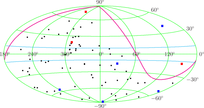
Figure 1: Distributions of 8 Fermi LAT AGN within $100\,{\rm Mpc}$ (blue and red squares) and 57 PAO UHECR (black bullets) in galactic coordinate using the Hammer projection. The red squares represent $\gamma$-ray emitting AGN in TeV band. The magenta line means a boundary of PAO field of view and the cyan lines represent the border of the low latitude region ($|b|<10^{\circ}$).

IV Statistical test method

To compare the arrival direction distribution expected from the model and that of the observed data, we need the method by which we can represent the characteristic of the distribution of arrival direction and apply the statistical test easily. We proposed some comparison methods in the previous paper Kim:2010zb ; Kim:2012en . In this analysis, we take the correlational angular distance distribution (CADD) method which is most appropriate for the test of the correlation between point sources and UHECR. CADD is the distribution of the angular distances between all pairs of the point source and UHECR arrival directions:

$$\hbox{CADD : }\left\{\theta_{ij^{\prime}}\equiv\arccos\,(\,\hat{\bf r}_{i}\cdot\hat{\bf r}^{\prime}_{j}\,)\;|\;i=1,\dots,N;\;j=1,\dots,M\right\},$$ (6)

where $\hat{\bf r}_{i}$ are the UHECR arrival directions, $\hat{\bf r}^{\prime}_{j}$ are the point source directions, and $N$ and $M$ are their total numbers, respectively. Now, we get two CADDs to compare: ${\rm CADD_{O}}$ from the observed UHECR and the $\gamma$-ray loud AGN, and ${\rm CADD_{M}}$ from the mock UHECR of the model under consideration and the same $\gamma$-ray loud AGN. The total number of the data in CADD is $N_{\rm CADD}=NM$, which means that the number of data in CADD are larger than the sampling number N.

By comparing ${\rm CADD_{O}}$ and ${\rm CADD_{M}}$, we can test whether our models are suitable to describe the observation. There are several statistical test methods which can prove that two distributions are different or not. One of the widely used statistical test methods is Kolmogorov-Smirnov (KS) test. It uses the KS statistic, which is the maximum absolute difference ($D_{\rm KS}$) between two cumulative probability distributions (CPD), CPD of the observed ${\rm CADD_{O}}$, $S_{O}(x)$, and that of the theoretically expected ${\rm CADD_{M}}$, $S_{M}(x)$,

$$D_{\rm KS}=\max_{x}\left|S_{O}(x)-S_{M}(x)\right|.$$ (7)

Once we calculate the KS statistic, we can get the probability that two different distributions come from the same population through the Monte-Carlo simulation. To get ${\rm CADD_{M}}$ accurately, we generates $10^{5}$ mock UHECR data. To obtain the probability distribution of the KS statistic $D_{\rm KS}$, we generate $10^{5}$ $D_{\rm KS}$ for a given model. Thus our probability estimation is reliable up to roughly $10^{-4}$.

V Results

In this work, we test 4 models for the UHECR sources: 1) the $\gamma$-ray loud AGN model with UHECR flux proportional to the inverse square of the distance, 2) the $\gamma$-ray loud AGN model with UHECR flux proportional to the $\gamma$-ray flux of AGN, 3) the TeV AGN model with UHECR flux proportional to the inverse square of the distance, and 4) the TeV AGN model with UHECR flux proportional to the $\gamma$-ray flux of AGN. From now on, we call them $\gamma$-d model, $\gamma$-f model, T-d model, and T-f model, respectively.

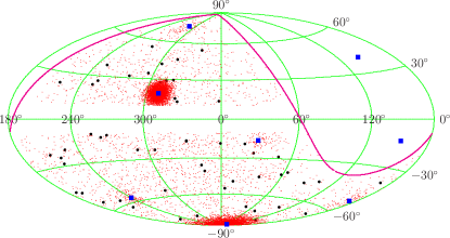
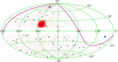
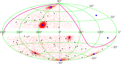
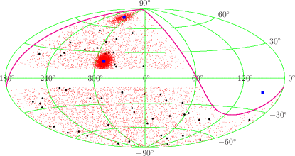
Figure 2: Distributions of the mock UHECR with smearing angle $\theta_{s}=6^{\circ}$ and AGN fraction $f_{A}=1$ (upper panels) and that of the mock UHECR with AGN fraction $f_{A}=0.7$ (lower panels). Left panels are for the $\gamma$-ray loud AGN model and right panels are for the TeV AGN model. The red dots are the mock UHECR generated by each AGN model and other marks are same with Fig. 1.

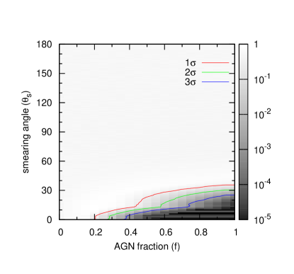
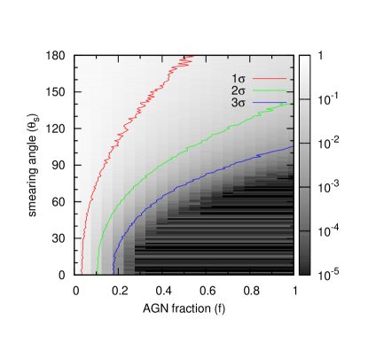
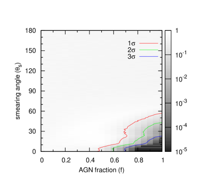
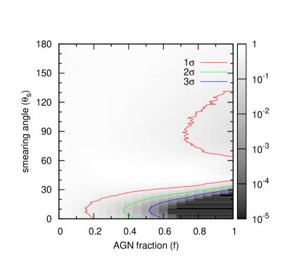
Figure 3: Probability dependencies on the AGN fraction ($f_{A}$) and the smearing angle $\theta_{s}$. The left panel is for $\gamma$-ray loud AGN model and the right panel is for TeV AGN model. The black gradient color means the probability and the solid lines represent the contour plot for $1\sigma$ (red), $2\sigma$ (green), and $3\sigma$ (blue).

Fig. 2 shows the distributions of the mock UHECR of 4 models with the smearing angle $\theta_{s}=6^{\circ}$ and the AGN fraction $f_{A}=0.7$. The two left panels are for the $\gamma$-ray loud AGN model, i.e., $\gamma$-d model (upper panel) and $\gamma$-f model (lower panel), and the two right panels are for the TeV AGN model, i.e., T-d model (upper panel) and T-f model (lower panel). The blue squares mark the locations of $\gamma$-ray loud AGN and the red dots represent mock UHECR generated from the source models. The mock UHECR concentrated near the AGN are generated from the source AGN and the uniformly distributed mock UHECR com from the isotropic background.

In Fig. 2, we can see the distinguished features depending on the source models we assumed. There are 6 $\gamma$-ray loud AGN in the field of view of PAO ($\gamma$-d model and $\gamma$-f model), and there are 2 TeV AGN among them (T-d model and T-f model). Also, we can see the difference in the mock UHECR distributions due to the difference in UHECR flux modeling. For the $\gamma$-d model, Cen A and NGC 0253 are the dominant sources because they are close to us. In contrast, for the $\gamma$-f model, 6 AGN contribute rather equally to the generation of mock UHECR. For the T-d model, Cen A is a dominant source, but Cen A and M87 share the proportion to generate the mock UHECR in the T-f model.

In Fig. 3, the probability of each model as a function of the AGN fraction from 0 to 1 and the smearing angle from $0^{\circ}$ to $180^{\circ}$ is given. The black gradient color represents the probability that the arrival direction distribution of the PAO UHECR comes from the given AGN source model. The red, green, and blue contours represent $1\sigma$, $2\sigma$, and $3\sigma$ probability lines.

First, let us compare the results of the $\gamma$-ray loud AGN models and TeV AGN models with UHECR flux proportional to the inverse square of the distance. Because the set of TeV AGN is a subset of $\gamma$-ray loud AGN, the principal difference between two models is the number of source AGN. It brings a significant difference in the results, which is shown in the upper panels in Fig. 3 ($\gamma$-d model and T-d model). As a rule of thumb, we choose the $3\sigma$ probability as a criterion for ruling out the model. The critical value of the AGN fraction is $f_{A,c}\sim 0.4$ and the critical value of the smearing angle is $\theta_{s,c}\sim 25^{\circ}$ for the $\gamma$-ray loud AGN model. Decreasing the AGN fraction from the critical value or increasing the smearing angle from the critical value increases the probability. In comparison, for the TeV model, the critical value of the AGN fraction is $f_{A,c}\sim 0.2$ and the critical value of the smearing angle is $\theta_{s,c}\sim 110^{\circ}$. We can deduce that it is hard to describe the observed UHECR distribution from T-d model.

Next, let us compare the results of two models with the same source AGN but with different UHECR flux models: the model which assumes that UHECR flux is proportional to the inverse square of the distance of source AGN and the model which assumes that UHECR flux is proportional to the $\gamma$-ray flux of source AGN. When we compare $\gamma$-d model to $\gamma$-f model, the critical values of the AGN fraction and the smearing angle are $f_{A,c}\sim 0.4$ and $\theta_{s,c}\sim 25^{\circ}$ for the $\gamma$-d model, and the critical values of the AGN fraction and the smearing angle are $f_{A,c}\sim 0.7$ and $\theta_{s,c}\sim 20^{\circ}$ for the $\gamma$-f model. We can exclude the AGN models in the cases having the parameters within the critical values (blue line). There is no crucial distinction between the different UHECR flux models for the $\gamma$-ray loud AGN models.

However, when we compare T-d model to T-f model, the different UHECR flux models result in the meaningful distinction. In the T-d model, Cen A is a dominant source to generate the mock UHECR, thus they are clustered around Cen A. Nevertheless, there is no significant difference among Cen A, M87, and NGC 1275 to produce the mock UHECR in the T-f model, thus the mock UHECR are clustered not only around Cen A but also around M87 and NGC 1275. This is the reason why the probability is increased dramatically as the smearing angle increases in the T-f model. The proportion of the mock UHECR produced by NGC 1275 which is located outside of the field of view increases as the smearing angle increases. Therefore, the clustered feature of the T-d model is quite different from the T-f model and the small number of source cause the clear discrepancy.

In short, we find that the source models assuming $\gamma$-ray loud AGN are responsible for UHECR ($\gamma$-d model and $\gamma$-f model) are more plausible than the source models assuming AGN having higher energy are responsible for UHECR (T-d model and T-f model). Also, which flux model is appropriate for describing the UHECR flux is not conclusive yet. This seems worthwhile to continue to study. At this stage, we can state the critical values that the null hypotheses are rejected. The critical regions are inside the $3\sigma$ contours. For the $\gamma$-d model, the critical values of the AGN fraction and the smearing angle are $f_{A,c}\sim 0.4$ and $\theta_{s,c}\sim 25^{\circ}$, and for the $\gamma$-f model, the critical values of the AGN fraction and the smearing angle are $f_{A,c}\sim 0.7$ and $\theta_{s,c}\sim 20^{\circ}$. The critical values are $f_{A,c}\sim 0.2$ and $\theta_{s,c}\sim 110^{\circ}$ in the case of the T-d model and the critical values are $f_{A,c}\sim 0.6$ and $\theta_{s,c}\sim 30^{\circ}$ in the case of the T-f model. That is, the $\gamma$-ray loud AGN dominance models with small smearing angle are excluded.

VI Discussion and Conclusion

The purpose of this work was to test the possibility of a subclass of AGN which emit strong $\gamma$-rays as the source of UHECR. We cannot confirm that the source model using $\gamma$-ray loud AGN is better than the source model using whole AGN in explaining the distribution of arrival direction of UHECR. Compared to the results of our previous work Kim:2012en , which assumes that whole AGN in the VCV catalog are the source of UHECR, the contour of $1\sigma$ is changed and the overall probability distribution for each hypothesis is higher than the previous results. (See the probability plot for the $\gamma$-d model and the left panel of Fig. 7 in Kim:2012en .) However, we cannot tell $\gamma$-ray loud AGN model describes the observation well definitely because the higher probabilities mean that the simulated distribution by models are consistent with the observed distribution only.

Nemmen et al. Nemmen:2010bp investigate the correlation of UHECR with $\gamma$-ray loud AGN using the first 27 PAO data and 1LAC. Since the data set and the constraints used in our work and those used in their work are different, we need to compare the results carefully. To test cross-correlation between PAO and 1LAC, they count the cumulative number of correlated UHECR as a function of angular distance from the 1LAC sources located within $200\,{\rm Mpc}$. They find that the angular distance $\psi\approx 17^{\circ}$ which minimizes the probability that the observed distribution would be the isotropic one. Although we pointed out that this method is not suitable to test the cross-correlation directly because it focuses on the deviation from isotropy rather than the direct correlation in the previous paper Kim:2010zb , the result is consistent with our results that $\gamma$-ray loud AGN dominance models having small smearing angle could be rejected.

The study of arrival direction of UHECR and its source could be one way of estimating the magnitude of the intervening magnetic fields or identifying the primary particle. If it is true that the $\gamma$-ray loud AGN could be the source of UHECR, the large smearing angle may imply the large deflections by intervening magnetic field. Interestingly, the larger deflection angles than traditional prediction ones are estimated by Ryu et al. Ryu et al. (2010), also. These may support the measurements of the shower maximum by PAO Abraham:2010yv — the primary particle is presumed to be heavy nuclei. In addition, the results by Dermer et al. Dermer:2010iz show that heavy nuclei are more likely to be accelerated to ultra-high energy in AGN. Taken together, it is possible that the primary particle would be heavy nuclei.

In summary, we tested the possibility that the $\gamma$-ray emitting AGN are the sources of UHECR. We took two sub-classes of AGN. One is the set of AGN emitting strong $\gamma$-rays observed by Fermi LAT and the other one is the subset of the former having $\gamma$-rays in TeV band. For the UHECR flux, we considered two possibilities: UHECR flux is proportional to the inverse square of the distance times the luminosity of its source and UHECR flux is proportional to the photon flux of AGN. We used UHECR with $E>55{\rm EeV}$ and based on GZK suppression, we restricted AGN to be within $d_{c}=100\,{\rm Mpc}$. Also, we introduced two free parameters in the simulation to produce the mock UHECR, AGN fraction $f_{A}$ and smearing angle $\theta_{s}$ so that we could manipulated the contribution of the source candidate and the deflection by intervening magnetic fields. To compare the distributions of observed UHECR to that of the mock UHECR, we adopted CADD which is suitable to test cross-correlation between UHECR and sources. The probabilities for 4 models calculated by KS test using CADD tells us that TeV AGN model with UHECR flux proportional to the inverse square of the distance is not appropriate to depict the observation. Rather, TeV AGN model with UHECR flux proportional to the photon flux is more plausible to describe the observation. In the cases of $\gamma$-ray loud AGN models, the effects of different flux models was not significant. If we reject the AGN models having the parameters within the $3\sigma$ contour, the critical values are $f_{A,t}\sim 0.4$ and $\theta_{s,t}\sim 25^{\circ}$ for the the $\gamma$-ray loud AGN models with UHECR flux proportional to the inverse square of the distance, and the critical values are $f_{A,t}\sim 0.7$ and $\theta_{s,t}\sim 20^{\circ}$ for the the $\gamma$-ray loud AGN models with UHECR flux proportional to the $\gamma$-ray flux. This means that the models having large isotropic background with $\gamma$-ray loud AGN or the $\gamma$-ray loud AGN dominance models with large deflection by the intervening magnetic fields make them possible to describe the observed UHECR. At this stage, it is hard to confirm that $\gamma$-ray loud AGN are the source of UHECR.

References

- (1) K. Greisen, Phys. Rev. Lett. 16, 748 (1966).
- (2) G. T. Zatsepin and V. A. Kuzmin, JETP Lett. 4, 78 (1966).
- (3) R. U. Abbasi et al. [The HiRes Collaboration], Phys. Rev. Lett. 100, 101101 (2008).
- (4) J. Abraham et al. [The Pierre Auger Collaboration], Phys. Lett. B 685, 239 (2010).
- (5) Y. Tsunesada [for the Telescope Array Collaboration], [arXiv:1111.2507 [astro-ph.HE]].
- (6) A. M. Hillas, Ann. Rev. Astron. Astrophys. 22, 425 (1984).
- (7) E. Waxman, Astrophys. J. 452, L1 (1995).
- (8) M. Vietri, Astrophys. J. 453, 883 (1995).
- (9) J. P. Rachen and P. L. Biermann, Astron. Astrophys. 272, 161 (1993).
- (10) F. Halzen and E. Zas, Astrophys. J. 488, 669 (1997).
- (11) M. Milgrom and V. Usov, Astrophys. J. 449, L37 (1995)
- (12) E. Waxman, Phys. Rev. Lett. 75, 386 (1995)
- (13) T. Stanev, R. K. Schaefer and A. A. Watson, Astropart. Phys. 5, 75 (1996)
- (14) D. F. Torres, E. Boldt, T. Hamilton and M. Loewenstein, Phys. Rev. D 66, 023001 (2002).
- (15) S. Singh, C. P. Ma and J. Arons, Phys. Rev. D 69, 063003 (2004).
- (16) D. S. Gorbunov, P. G. Tinyakov, I. I. Tkachev and S. V. Troitsky, JETP Lett. 80, 145 (2004).
- (17) R. U. Abbasi et al. [HiRes Collaboration], Astrophys. J. 636, 680 (2006).
- (18) R. U. Abbasi et al., Astropart. Phys. 30, 175 (2008).
- (19) J. Abraham et al. [Pierre Auger Collaboration], Science 318, 938 (2007).
- (20) P. Abreu et al. [Pierre Auger Collaboration], Astropart. Phys. 34, 314 (2010).
- (21) H. B. Kim and J. Kim, JCAP 1103, 006 (2011).
- (22) H. B. Kim and J. Kim, arXiv:1203.0386 [astro-ph.HE].
- (23) M.-P. Véron-Cetty and P. Véron, Astron. Astrophys. 455, 773 (2006).
- (24) M.-P. Véron-Cetty and P. Véron, Astron. Astrophys. 518, A10 (2010).
- (25) D. Harari, S. Mollerach and E. Roulet, Mon. Not. Roy. Astron. Soc. 394, 916 (2009).
- (26) M. R. George et al. Mon. Not. Roy. Astron. Soc. 388, L59 (2008).
- (27) R. S. Nemmen, C. Bonatto and T. Storchi-Bergmann, Astrophys. J. 722, 281 (2010).
- (28) Y. Y. Jiang et al. Astrophys. J. 719, 459 (2010).
- (29) The Fermi-LAT Collaboration, Astrophys. J. 743, 171 (2011).
- (30) C. D. Dermer and S. Razzaque, Astrophys. J. 724, 1366 (2010).
- (31) The Fermi-LAT Collaboration, Astrophys. J. 715, 429 (2010)
- (32) T. Kashti and E. Waxman, JCAP, 0805, 006 (2008)
- (33) H. B. J. Koers and P. Tinyakov, JCAP, 0904, 003 (2009)
- (34) P. Sommers, Astropart. Phys. 14, 271 (2001)
- (35) M, A. Stephens, J. Royal Stat. Soc. B, 32, 115 (1970)
- Ryu et al. (2010) D. Ryu, S. Das, and H. Kang, ApJ, 710, 1422 (2010)
- (37) J. Abraham et al. [Pierre Auger Collaboration], Phys. Rev. Lett. 104, 091101 (2010)