Simulating lattice spin models on GPUs

Abstract

Lattice spin models are useful for studying critical phenomena and allow the extraction of equilibrium and dynamical properties. Simulations of such systems are usually based on Monte Carlo (MC) techniques and the main difficulty often being the large computational effort needed when approaching critical points. In this work it is shown how such simulations can be accelerated with the use of NVIDIA Graphics Processing Units (GPUs) using the CUDA programming architecture. We have developed two different algorithms for lattice spin models, the first useful for equilibrium properties near a second order phase transition point and the second for dynamical slowing down near a glass transition. The algorithms are based on parallel MC techniques and speedups from 70 to 150 fold over conventional single-threaded computer codes are obtained using consumer-grade hardware.

I Introduction

In most common cases, computer programs are written serially: to solve a problem, an algorithm is constructed and implemented as a serial stream of coded instructions. These instructions are executed on a Central Processing Unit (CPU) on one computer. Momentarily disregarding specific cases for which modern CPU hardware is optimized, only one instruction may be executed at a time; on its termination, the next instruction begins its execution. On the other hand, parallel computing involves the simultaneous use of multiple computational resources. In recent years, massively parallel computing has become a valuable tool, mainly due to the rapid development of the Graphics Processing Unit (GPU), a highly parallel, multi-threaded, many core processor. However, due to the specialized nature of the hardware, the technical difficulties involved in GPU programming for scientific use stymied progress in the direction of using GPUs as general-purpose parallel computing devices. This situation has begun to change more recently, as NVIDIA introduced $\text{CUDA}^{\text{TM}}$, a general purpose parallel computing architecture with a new parallel programming model and instruction set architecture (similar technology is also available from ATI but was not studied by us). CUDA comes with a software environment that allows developers to use C (C++, CUDA FORTRAN, OpenCL, and DirectCompute are now also supported NVIDIA CUDA^TM (2010, http://www.nvidia.com/object/cuda_develop.html (accessed 7/2010)) for program development, exposing an application programming interface and language extensions that allow access to the GPU without specialized assembler or graphics-oriented interfaces. Nowadays, there are quite a few scientific applications that are running on GPUs; this includes quantum chemistry applications Ufimtsev and Martinez (2008, 2009), quantum Monte Carlo simulations Anderson et al. (2007); Meredith et al. (2009), molecular dynamicsvan Meel et al. (2007); Stone et al. (2007); Anderson et al. (2008); Davis et al. (2009); Friedrichs et al. (2009); Genovese et al. (2009); Dematt$\grave{{e}}$ and Prandi (2010); Eastman and Pande (2010), hydrodynamics Bernaschi et al. (2010), classical Monte Carlo simulations Lee et al. (2009); Preis et al. (2009); Block et al. (2010), and stochastic processes Juba and Varshney (2008); Januszewski and Kostur (2010); Balijepalli et al. (2010).

In this work we revisit the problem of parallel Monte Carlo simulations of lattice spin models on GPUs. Two generic model systems were considered:

1. The two-dimensional (2D) Ising model Onsager (1944) serves as a prototype model for describing critical phenomena and equilibrium phase transitions. Numerical analysis of critical phenomena is based on computer simulations combined with finite size scaling techniques Newman and Barkema (1999). Near the critical point, these simulations require large-scale computations and long averaging, while current GPU algorithms are limited to small lattice sizes Preis et al. (2009) or to spin $\frac{1}{2}$ systems Block et al. (2010). Thus, in three-dimensions (3D), the solution of lattice spin models still remains a challenge in statistical physics.

2. The North-East model Reiter et al. (1992) serves as a prototype for describing the slowing down of glassy systems. The computational challenge here is mainly to describe correlations and fluctuations on very long timescales, as the system approaches the glass temperature (concentration) Reiter et al. (1992). As far as we know, simulations of facilitated models on GPUs have not been explored so far, but their applications on CPU has been discussed extensively Garrahan and Chandler (2003); Jack et al. (2006); Garrahan et al. (2007); Chandler and Garrahan (2010).

We develop two new algorithms useful to simulate these lattice spin models. For certain conditions, we obtain speedups of two orders of magnitude in comparison with serial CPU simulations. We would like to note that in many GPU applications, speedups are reported in Gflops, while in the present work, we report speedups of the actual running time of the full simulation. The latter provides a realistic estimate of the performance of the algorithms.
The paper is organized as follows: Section II comprises a brief introduction to GPUs and summarizes their main features. Section III contains a short overview of lattice spin models and the algorithms developed. Section IV includes a short discussion of the random number generator used in this work. Section V presents the results and the comparisons between CPU and GPU performance. Finally, Section VI concludes.

II GPU architecture

In order to understand GPU programming we provide a sketch of NVIDIA’s GPU device architecture. This is important for the development of the algorithms reported below, and in particular for understanding the logic and limitations behind our approach. By now three generations of GPUs have been released by NVIDIA (G$80$, GT$200$ and the latest architecture codename “Fermi”). In table 1 we highlight the main features and differences between generations.

II.1 Hardware specifications

On a GPU device one finds a number of Scalar Multiprocessors (SMs). Each multiprocessor contains $8/32$ (architecture dependent) Scalar Processor cores (SPs), a Multi-threaded Instruction Unit (MTIU), special function units for transcendental numbers and the execution of transcendental instructions such as sine, cosine, reciprocal, and square root, $32$-bit registers and the shared memory space. In general, unlike a CPU, a GPU is specialized for compute-intensive, highly parallel computation - exactly the task graphics rendering requires - and is therefore designed such that more transistors are devoted to data processing rather than data caching and flow control. This is schematically illustrated in figure 1, and makes GPUs less general-purpose but highly effective for data-parallel computation with high arithmetic intensity. Specifically, they are optimized for computations where the same instructions are executed on different data elements (often called Single Instruction Multiple Data, or SIMD) and where the ratio of arithmetic operations to memory operations is high. This puts a heavy restriction on the types of computations that optimally utilize the GPU, but in cases where the architecture is suitable to the task at hand it speeds up the calculations significantly.

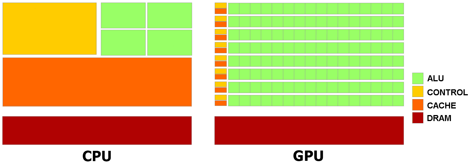
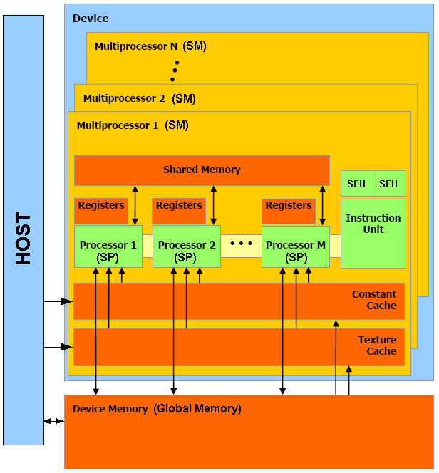
Figure 1: (a) A schematic delineation that illustrates the ratio of transistors devoted to data processing (ALUs) to those of data caching and flow control in CPUs and GPUs. This is a manifestation of the different philosophies between the “all purpose” CPU to the “dedicated purpose” GPU. (b) A visual hardware model that describes the memory architecture and hierarchy of a GPU device. (Courtesy of NVIDIA).

II.2 Memory architecture

NVIDIA’s GPU memory model is highly hierarchical and is divided into several layers:

Registers:

The fastest form of memory on the GPU. Usually automatic variables declared in a kernel reside in registers, which provide very fast access.

Local Memory:

Local memory is a memory abstraction that implies “local” in the scope of each thread. It is not an actual hardware component of the SM. In fact, local memory resides in device memory allocated by the compiler and delivers the same performance as any other global memory region.

Shared memory:

Can be as fast as a register when there are no bank conflicts or when reading from the same address. It is located on the SM and is accessible by any thread of the block from which it was created. It has the lifetime of the block (which will be defined in the next subsection).

Global memory:

Potentially about $400-600$ times slower than register or shared memory. This module is accessible by all threads and blocks. Data transfers from and to the GPU are done from global memory.

Constant memory:

Constant memory is read only from kernels and is hardware optimized for the case when all threads read the same location(i.e. it is cached). If threads read from multiple locations, the accesses are serialized.

Texture memory:

Graphics processors provide texture memory to accelerate frequently performed operations. The texture memory space is cached. The texture cache is optimized for $2\mbox{D}$ spatial locality, so threads of the same warp that read texture addresses that are close together will achieve best performance. Constant and texture memory reside in device memory.

II.3 CUDA programing model

As has been mentioned, CUDA includes a software environment that allows developers to develop applications mostly in the C programming language. C for CUDA extends C by allowing the programmer to define C functions (kernels) that, when called, are executed $N$ times in parallel by $N$ different CUDA threads on the GPU scalar processors. Before invoking a kernel, the programmer needs to define the number of threads ($N$) to be created. Moreover the programmer needs to decide into how many blocks these threads will be divided. When the kernel is invoked, blocks are distributed evenly to the different multiprocessors (hereby, having $p$ multiprocessors, requires a minimum of $p$ blocks to achieve $100\%$ utilization of the GPU). The blocks might be $1$, $2$ or $3$ dimensional with up to $512$ threads per block. Blocks are organized into a $1$ or $2$ dimensional grid containing up to $65,535$ blocks in each dimension. Each of the threads within a block that execute a kernel is given a unique thread ID. To differentiate between two threads from two different blocks, each of the blocks is given a unique ID as well. Threads within a block can cooperate among themselves by sharing data through shared memory. Synchronizing thread execution is possible within a block, but different blocks execute independently. Threads belonging to different blocks can execute on different multiprocessors and must exchange data through the global memory. There is no efficient way to synchronize block execution, that is, in which order or on which multiprocessor they will be processed, thus, an efficient algorithm should avoid communication between blocks as much as possible.
Much of the challenge in developing an efficient GPU algorithm involves determining an efficient mapping between computational tasks and the grid/block/thread hierarchy. The multiprocessor maps each thread to one scalar processor, and each thread executes independently with its own instruction address and register state. The multiprocessor SIMT (Single Instruction Multiple Threads) unit creates, manages, schedules, and executes threads in groups of $32$ called warps. When a multiprocessor is given one or more thread blocks to execute, it splits them into warps that get scheduled by the SIMT unit. The SIMT unit selects a warp that is ready to execute and issues the next instruction to the active threads of the warp. A warp executes one common instruction at a time, so full efficiency is realized when all threads of a warp agree on their execution path (on the G$80$ and GT$200$ architectures, it takes 4 clock cycles for a warp to execute, while on the Fermi architecture it takes only one clock cycle). If threads of a warp diverge via a data dependent conditional branch, the warp serially executes each branch path taken, disabling threads that are not on that path. When all paths terminate, the threads converge back to the same execution path. Branch divergence occurs only within a warp: different warps execute independently regardless of whether they are executing common or disjointed code paths. More information can be found in Ref.NVIDIA CUDA^TM (2010, http://www.nvidia.com/object/cuda_develop.html (accessed 7/2010).

	G80	GT200	Fermi
Maximum number of multiprocessors	16	30	16
Scalar cores per multiprocessor	8	8	32
Double precision capability	none	30 FMA ops/clock	256 FMA ops/clock
Special function units	2	2	4
Warp schedulers per multiprocessor	1	1	2
Shared memory	16 KB	16 KB	48 KB
Concurrent kernels	1	1	Up to 16

Table 1: Summary of NVIDIA’s different architectures

III Lattice spin models

We consider a general lattice model of spins that are placed on a square lattice of dimensions $d=1,2,3...$. The spins may be of any dimension and may acquire continuous or discrete values. In the applications reported below, we focus, for simplicity, on the case where the spins at lattice site $i$ take discrete values of $s_{i}=\pm 1$, but this can be easily extended to any spin dimension and value. The interactions between the spins is given by the Hamiltonian:

$$H=\sum_{i\neq j}J_{ij}s_{i}s_{j}+\sum_{i}B_{i}s_{i}.$$ (1)

In the above equation, the first sum is usually carried over nearest neighbors only (which we will denote $\langle ij\rangle$). $J_{ij}$ is the interaction parameter and may be constant, discrete or continuous and $B_{i}$ is an external field. The above Hamiltonian can be used to study equilibrium properties as in the Ising model and spin glass models (Edwards-Anderson model Edwards and Anderson (1975), Sherrington-Kirkpatrick model Sherrington and Kirkpatrick (1975), random orthogonal model Marinari et al. (1994) etc.), or the dynamic behavior as in facilitated spin models (Fredrickson and Andersen Fredrickson and Andersen (1984), Jackle-Eisinger north-east model Jäckle and Eisinger (1991); Reiter et al. (1992), etc.). Simulations of such systems are based on Monte Carlo techniques Landau and Binder (2000). In most CPU implementations, the algorithms for equilibrium or dynamic simulations do not differ significantly. However, as will become clear below, they become very different when implemented on a GPU. Though the implementations described below are for two simple cases, the extension of our approach to the spin glass models mentioned above or to other facilitated spin models is straightforward.

III.1 Monte Carlo simulation of the 2D Ising model

The simplest $2\mbox{D}$ Ising model Newman and Barkema (1999) describes$N$ magnetic dipoles (or spins) placed on a $2\mbox{D}$ square lattice with one spin per cell. We limit the discussion to the spin $\frac{1}{2}$ case, where each spin has only two possible orientations, “up”and “down”. Each spin interacts with its nearest neighbors only, with a fixed interaction strength. In the absence of an external magnetic field, the Hamiltonian is given by

$$H=-J\sum_{\langle ij\rangle}s_{i}s_{j},$$ (2)

where $\langle ij\rangle$ represents a sum over nearest neighbors and $J$ determines the energy scale. Monte Carlo simulation techniques based on the Metropolis algorithm Metropolis et al. (1953) are perhaps the most popular route to obtain the thermodynamic properties of this model. In a CPU implementation of the Metropolis algorithm, a spin is selected at random and an attempt to flip the spin is accepted with the Metropolis probability $P_{acc}=\min[1,\exp(-\Delta H/T)]$, where $T$ is the temperature in units of energy. In the GPU algorithm developed here, we will take advantage of the fact that spins interact only with their nearest neighbors, and thus the problem can be divided into non-interacting domains. The generalization to the case of finite interacting regions is straightforward. The algorithm is as follows:

1. Randomly initialize the lattice (this is done on the CPU).

2. Copy lattice to the GPU.

3. Divide the lattice into $Q$ sub-lattices, each with $P$ spins.

4. A grid of $Q$ thread-blocks is formed. Every thread-block contains $\frac{P}{4}$ threads.

5. Every block copies a sub-lattice including its boundaries from the global memory to the shared memory. To avoid bank conflicts and save precious shared memory space, the short data type was used to form the lattice (figure 2).

6. Within the block, every thread is in charge of $4$ spin sites (a sub block of $2\times 2$). At first all red spins are updated (figure 3), i.e. all threads are active. Once a thread finished updating the red spin it continues to update its blue spin (figure 3). Since no native block synchronization exists, before updating the remaining spins, we make sure that all blocks finished the first two steps. This is done by recopying the data from the shared memory (boundaries excluded) on to the global memory and ending the kernel.

7. Relaunch the kernel with the configuration generated in the previous step. Redo steps $5$ and $6$, only this time the green and white spins are being updated (figure 3).

8. Recopy data to global memory.

This completes one Monte Carlo step (or one lattice sweep). In our implementation we chose sub-lattices of $32\times 32$ in size and blocks of $256$ threads, as this choice turned out to be the most efficient. Using more threads does in fact reduce the time it takes the block to copy a sub-lattice to the shared memory, but then the ratio of arithmetic operations to memory operations is low and performance is poor. To obtain thermodynamic average properties, we use the fact the CPU and GPU can work in parallel and the lattice is copied from the device to the host from time to time, so averages can be calculated on the CPU while the GPU continues to sweep the lattice. We note in passing that similar algorithms have been proposed by Tobias et al. Preis et al. (2009) and Blocket al..Block et al. (2010) The former approach is restricted to lattices with up to $1024\times 1024$ spins in 2D (assuming spins are stored as integer data type), whereas the algorithm presented in this work is applicable to larger systems, is designed for coalesced global memory access and avoids bank conflicts, all of which makes better use of the GPU architecture. The limit of system size in our approach is related to the size of the global memory on the GPU, which is typically on the order of $1-4\mbox{GB}$. This amounts to maximum system sizes of $20,000\times 20,000$ - $40,000\times 40,000$ spins. The algorithm of Block et al. Block et al. (2010) is applicable to much larger systems and deals with the issue of multi-GPU programming, but is currently restricted to spin $\frac{1}{2}$ systems while the algorithm presented in this work is suitable for the more generalized Potts modelWu (1982) and gives approximately the same speedups in comparison to an equivalent CPU code.

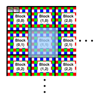
Figure 2: Illustration of the algorithm for an Ising model implemented on a GPU device. Every block handles a sub lattice. Every thread is assigned $4$ spin sites according to its ID and block. In order to improve memory access each block copies its sub-lattice on to shared memory. Since a spin needs its 4 nearest neighbors to update, extra boundary sites are copied as well (blueish square).

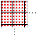
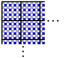
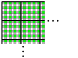
Figure 3: As native block synchronization is not available on a GPU, one must end the kernel in order to achieve it. This is only necessary after the red and blue spin where updated (as can be clearly seen, they do not interact) and before moving on to the green and white spins, which in turn do interact with the aforementioned updated red and blue spins.

To acquire the correct thermodynamic equilibrium state, the chosen set of Monte Carlo moves must satisfy either detailed balance or the weaker balance condition. On the CPU detailed balance is rigorously satisfied when randomly selecting a spin within the Metropolis algorithm. For the GPU, however, the approach we developed breaks detailed balance and only balance is satisfied Manousiouthakis and Deem (1999); Ren and Orkoulas (2006). This is a sufficient condition to ensure that the algorithm describes the correct Boltzmann distribution.

III.2 The North-East model

The North-East model is based on the Ising model Hamiltonian with special constraints that are used to model facilitated dynamics Fredrickson and Andersen (1984); Nakanishi and Takano (1986); Reiter et al. (1992). The Hamiltonian is given by:

$$H=J\sum_{\left\langle i,j\right\rangle}s_{i}s_{j}+B\sum_{i}s_{i},$$ (3)

where $s_{i}$, $J$, $B$ and $\langle ij\rangle$ are described above. What makes this model different from the previous one is a constraint imposed on the transition probability to flip a spin. This probably is zero unless the spin’s upper (north) and right (east) neighbors point “up”. In the latter case, one accepts a flip with the same Metropolis probability given by $P_{acc}=\min[1,\exp(-\Delta H/T)]$. Thus, the thermodynamics of the model are the same as the Ising model, but the Monte Carlo dynamics generated by the above rule is quite different. In most applications reported in the literature one takes $J=0$. For $J\neq 0$ the dynamics generated by this model are richer and show an interesting re-entrant transition Geissler and Reichman (2005). When $J=0$ the thermodynamics are trivial and the coupling between neighboring spins depends only on the aforementioned dynamical constraint. The lattice is initialized so spins point “up” with the probability $c$, which is also the equilibrium density of spins pointing “up”, and can be expressed as $c=\frac{1}{z}e^{-1/T}$, where the partition function is $z=e^{1/T}+e^{-1/T}$ and $T$ is the unit-less temperature. Due to the dynamical constraints, if $c$ is too low, one finds domains of spins that are stuck. For a high values of $c$ on the other hand, all spins are flippable. As a consequence, there is a critical concentration $c^{*}$ below which the system is not ergodic. This transition from ergodic to non-ergodic behavior is modeled by the spin-spin autocorrelation function

$$\Phi(t)=\sum_{i}\frac{\left\langle s_{i}(t)\cdot s_{i}(0)\right\rangle-\left\langle s_{i}\right\rangle^{2}}{1-\left\langle s_{i}\right\rangle^{2}},$$ (4)

where $\langle s_{i}\rangle=2c-1$ is the average spin polarization and $s_{i}(t)$ is the spin polarization at Monte Carlo step $t$ for site $i$. We expect the function to decay to zero for an initial concentration $c>c^{*}$ and to decay to a finite value $f$ (which is the fraction of spins that are stuck) for $c<c^{*}.$ The CPU implementation of the North-East model is identical to that described for the Ising model, with the additional constraint for the flipping probability.
The GPU implementation for this model, similar as it may seem to the Ising model, is a bit cannier. We found out that applying the checkerboard algorithm (described in subsection III.1) does not yield the same relaxation dynamics as the serial CPU implementation. This is understandable, since this model imitates a diffusion process: for a spin to be able to change its configuration it is necessary that its north and east neighbors point up. If they do not, they in turn will also need their neighbors to point up to be able and change their configuration. Equilibration takes place by an up spin diffusion from “north-east” to “south-west”. By sequentially (instead of randomly) sweeping the lattice we change the dynamics of this process. Such being the case, the corrected algorithm we developed is:

1. Initialize the lattice so spins point up with probability $c$ (on the CPU).

2. Copy lattice to the GPU.

3. Divide the lattice into $Q$ sub-lattices, each with $P$ spins.

4. A grid of $Q$ thread-blocks is formed. Every thread-block contains $\frac{P}{4}$ threads.

5. Blocks then randomly pick a sub-lattice (figure 4) in such a way that two different blocks cannot pick the same sub-lattice. Every block copies a sub-lattice including its boundaries from the global memory to the shared memory.

6. Within each block, $\lambda$ threads concurrently pick $\lambda$ spins from the sub-lattice randomly and update them. $\lambda$ is chosen to be a small fraction of $P$.

7. Synchronize the block.

8. Reiterate steps $6-7$ $q$ times, such that $q\cdot\lambda=\frac{P}{2}$.

9. Copy back data from shared memory to global memory (to allow block synchronization).

10. Relaunch the kernel with the same configuration and redo steps $5-8$.

11. Recopy data to global memory.

This completes one lattice sweep. Again we use the fact the CPU and GPU can work in parallel, and the lattice is copied from the device to the host from time to time to store the spin’s configuration for the computation of the autocorrelation function.
The algorithm presented here does not preserve detailed balance nor the weaker balance condition, but since we are interested in its dynamics the given algorithm is correct. One should note that in order to obtain the correct dynamics an initialization of the parameter $\lambda$ is needed. It is obvious that in the limit where $Q=\lambda=1$ the algorithm is in fact serial and preserves detailed balance (results for this limit are given by the black line in figure 5). We can now use this result as a reference, and increase the number of threads and blocks that are working in parallel. There is an upper limit above which the results will diverge from the desired reference and the dynamics will no longer be correctly reproduced. Once $\lambda$ has been evaluated, the simulation can be performed. In figure 5 we provide a consistent test on the value of $\lambda$ for the North-East model at $c=0.42$.

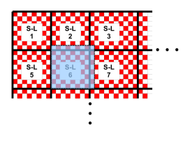
Figure 4: Although the figure above looks similar to the Ising model implementation, in this case Sub-lattices and spins are chosen randomly. This preserves the dynamical behavior in comparison to CPU algorithms. Note that when copying the data to the shared memory, only the upper and right boundaries are necessary.

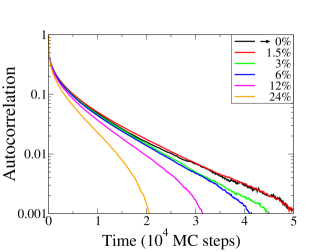
Figure 5: Convergence tests of the parameter $\lambda$ for the North-East model at $c=0.42$. The solid black line represents the reference value, which was obtained by running the simulation on a single thread - single block. This result is identical to the serial CPU result. The best performence is achieved for sub-lattices of $32\times 32$ spins and for $\lambda=16$ threads, i.e., attempts to flip only $\sim 1.5\%\approx\frac{16}{32\times 32}$ of the spins inside a sub-lattice. One can see that for higher values of $\lambda$, the correlation diverges from the correct result.

It is possible to write an algorithm that maintains the weaker balance condition and at the same time preserve the dynamical relaxation of the model. The drawback of such an algorithm, however, is that it is $\approx 2.5\times$ slower then the one presented above. The only changes are in steps $6-9$:

1. Within each block, $\lambda$ threads concurrently pick $\lambda$ red spins (figure 4) from the sub-lattice randomly and update them. $\lambda$ is chosen to be a small fraction of $P$.

2. Synchronize the block and pick $\lambda$ white spins from the sub-lattice randomly and update them.

3. Copy back data from shared memory to global memory (to allow block synchronization).

4. Relaunch the kernel with the same configuration and redo steps $6-8$ three more times (this will complete one MC step).

IV Pseudo random numbers generation

Monte Carlo simulations rely heavily on the availability of random or pseudo-random numbers. In this work, random numbers were used to determine whether spin flips are accepted or rejected, in accordance with the Metropolis algorithm. As is widely known, the use of a poor quality PRNG (Pseudo Random Numbers Generator) may lead to inaccurate simulations.Ferrenberg et al. (1992) In the course of this work three different PRNGs were utilized:

1. L’Ecuyer with Bays-Durham shuffle and added safeguards.Press et al. (1992) This PRNG has a long period ($2\times 10^{18}$) and is easy to implement on a CPU. Unfortunately, porting it to GPUs causes a dramatic decrease in performance: this is mostly due to the fact that the implementation of this algorithm requires too many registers.

2. The "minimal" random number generator of Park and Miller.Press et al. (1992) This PRNG has a period of $2\times 10^{9}$ and is portable to GPUs. In practice, however, it proved to work poorly and the GPU simulation results were in poor agreement with reference values obtained with better PRNGs.

3. Linear Congruential Random Number Generator (LCRNG).Press et al. (1992) This PRNG has a period of $10^{6}-10^{9}$ and provided good results even for very long runs. The LCRNG algorithm is very easy to port to the GPU and has the advantage of being very fast, requiring only a few operations per call.

In our implementations (section III), each thread used a separate LCRNG, creating its own sequence of pseudo-random numbers with a unique seed. The sequence (of thread $i$) is created as follows:

$$x_{j+1}^{Th_{i}}=\left(a\cdot x_{j}^{Th_{i}}+c\right)\mbox{{mod}}\ m$$ (5)

$$x_{j+1}^{Th_{i}}=\mbox{abs}\left(\frac{x_{j+1}^{Th_{i}}}{2^{31}}\right)$$ (6)

An appropriate choice of the coefficients is responsible for the quality of the LCRNG. We used Press et al. (1992) $a=1,664,525$ , $c=1,013,904,223$ and $m=2^{32}$. The different seeds were created per thread according to

$$x_{0}^{Th_{i+1}}=\left(16807\cdot x_{0}^{Th_{i}}\right)\mbox{{mod}}\ m$$ (7)

with $x_{0}^{Th_{0}}=1$. Similar PRNGs were used for other GPU applications.Preis et al. (2009); Block et al. (2010)

V Results

For comparison, CPU codes were executed on a PC with Intel Core2 Duo E7400 @ $2.8G\mathrm{Hz}$ processor, Intel RaisinCity motherboard with Intel G41 chipset and Kingstone $2\mathrm{GB},\,800\mathrm{MHz}$ RAM (only a single core was used for the calculations). The operating system was CENTOS. Codes were compiled with Intel C++ compiler (ICC) using all optimizations provided for best performance. Speedups reported here are given in terms of the complete application running time (from initialization till results are processed), rather than Gflops or spin updates per second. This choice is important, as it most closely describes the “real” gain in practical simulations by the use of a GPU rather than a CPU.

V.1 Ising model

In order to verify the GPU implementation, we compared values of magnetization, energy and heat capacity as a function of temperature (temperature was taken in energy units) between GPU and CPU versions. In figure 6 results from a $128\times 128$ spin lattice are presented. We find the results to clearly agree. In terms of acceleration we achieved a $15\times$ factor for lattices with $512\times 512$ spins on the GT $9600$ GPU (G$80$ architecture). Implementing the same code on the new GTX $480$ GPU, we achieved a factor of $150\times$. This factor reduces to $2\times$ for small lattices ($32\times 32$). The reason for this is that in small problems it becomes harder to hide memory access latencies, because there are not enough threads to execute between memory access operations. A theoretical analysis of our implementation shows that the GPU reaches full occupancy (a useful tool to check this is the “CUDA GPU Occupancy Calculator” which can be freely downloaded from Ref.Occ ). The $10$ fold factor obtained by the GTX $480$ in comparison with the GT $9600$ is easily understood when taking into consideration that the GTX $480$ has$15$ SMs instead of $8$ (on the GT $9600$), $4$ blocks can be active simultaneously instead of $3$ and a warp executes in one clock cycle instead of $4$. Thus the relative speedup is $\frac{15}{8}\cdot\frac{4}{3}\cdot\frac{4}{1}=10$. From figure 8 it is obvious that the GPU reaches full occupancy only for lattices bigger than $128\times 128$. Note also that near the critical temperature, the fluctuations and noise increase. Since the present work is not concerned with determining the critical behavior, we have used the same number of Monte Carlo sweeps for all temperatures. Estimation of the critical behavior requires much longer runs, and perhaps also larger systems. In this respect, the GPU approach developed here provides the means to increase numerical accuracy by more than one order of magnitude (noise scales with the square root of the number of MC steps), either by increasing the system size or by simulating longer Monte Carlo runs.

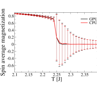
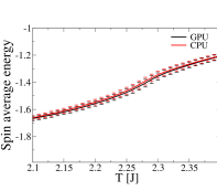
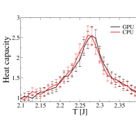
Figure 6: Comparison between the Monte Carlo simulation done on a CPU and on a GPU for a $128\times 128$ spin lattice. The temperature was stepwise reduced by $0.01$ from $T=2.4$ to $T=2.1$. The critical temperature for this model is $T_{c}=2/\log(1+\sqrt{2})$. At each temperature, $2\times 10^{7}$ sweeps through the lattice were performed, during which $10,000$ different measurement were taken (after reaching equilibrium). In (a) we show the average spin magnetization, in (b) the average spin energy and in (c) the heat capacity.

V.2 North-East model

The North-East model has a critical concentration $c^{*}\approx 0.3$, below which the dynamics break ergodicity. In figure 7 we show the results for spin-spin autocorrelation function for different concentrations above the critical value. Two lattice sizes were studied. Similar to the previous case, we find that the GPU results agree well with the CPU results, indicating that the proposed algorithm reproduces the correct dynamics. This is not trivial and depends on the value chosen for $\lambda$. Moreover, as pointed out above, the algorithm used for the Ising model fails to produce correct relaxation times. As the system approached the critical concentration the dynamics become sluggish and the autocorrelation function decays slowly to zero.

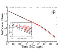
(a) $c=0.32$, Time$=10^{8}$

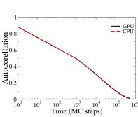
(b) $c=0.37$, Time$=10^{6}$

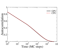
(c) $c=0.42$, Time$=10^{5}$

Figure 7: Comparison between spin-spin autocorrelation functions calculated from simulations done on a CPU and on a GPU for spin lattices of different sizes and different initial concentrations. Results were obtained by averaging the autocorrelation functions of $30$ different initial realization for every concentration. (a) Results for a $128\times 128$ spin lattice. As can be seen for low concentrations approaching $c^{*}$, relaxation time is very long (longer than the time we were willing to wait for the CPU results). Furthermore, at this concentration, more than 30 trajectory are required to average the autocorrelation function. (b) and (c) Results obtained from $512\times 512$ spin lattices.

In figure 8 we compare the running times between the CPU and two GPU architectures. We achieved a $2\times$ factor on the GT $9600$ GPU and a $\approx 70\times$ speedup running the same code on the new GTX $480$ GPU. This factor reduces to $8\times$ for smaller lattices ($128\times 128$ and less). The GPU acceleration is nearly two orders of magnitude, implying that one can simulate the system closer to the critical density. This is important, since the behavior of relaxation near the critical density is not necessarily universal, and thus extrapolations are often tricky.

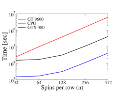
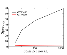
Figure 8: (a) Processing times for the 2D Ising model. Times are shown as a function of the number of spins $n$ per row which is related to the system size by $N=n^{2}$. A maximum acceleration factor of $15$ was achieved (on the GT 9600GPU). We believe a higher value can be obtained for larger lattices. (b) Speedups of two different GPU cards versus the CPU serial implementation for the North-East model. Again times are shown as a function of the number of spins $n$ per row.

VI Conclusions and Summary

We have developed algorithms to simulate lattice spin models on consumer-grade GPUs. Two prototype models have been considered: The Ising model describing critical phenomena at equilibrium and the North-East model describing glassy dynamics. We showed that for equilibrium properties of lattice models an impressive speedup of $150\times$ can be achieved. To simulate the dynamics of such models, a more sophisticated approach was developed in order to preserve the dynamical rules and outcome. Our algorithm for the dynamic model reaches a $\approx 70\times$ factor in comparison to the serial CPU implementation for large system sizes. Though the algorithms were performed on specific models, we feel they can be easily extended to a larger class of similar systems.
Since the gain in computational power embodied by these results is in some cases two orders of magnitude, while the required GPU hardware is priced similarly to a CPU and can often be added to existing systems, the algorithms are certainly of interest. On the other hand, taking full advantage of it still requires savvy knowledge of the device and its capabilities and limitations, and the development of specific numerical algorithms. As the advantages of this useful technology become clear and knowledge about its implementation continues to build up and spread, we hope it will become more accessible to a wide variety of computationally-minded scientists.

VII Acknowledgments

We would like to thank Prof. Sivan Toledo for discussions. This work was supported by the Israel Science Foundation (grant no. 283/07). GC is grateful to the Azrieli Foundation for the award of an Azrieli Fellowship. ER thanks the Miller Institute for Basic Research in Science at UC Berkeley for partial financial support via a Visiting Miller Professorship.

References

- NVIDIA CUDATM (2010, http://www.nvidia.com/object/cuda_develop.html (accessed 7/2010) NVIDIA CUDATM, Compute Unified Device Architecture Programming Guide Version 3.0; 2010, http://www.nvidia.com/object/cuda_develop.html (accessed 7/2010).
- Ufimtsev and Martinez (2008) Ufimtsev, I. S.; Martinez, T. J. CiSE 2008, 10, 26–34.
- Ufimtsev and Martinez (2009) Ufimtsev, I. S.; Martinez, T. J. J. Chem. Theory Comput. 2009, 5, 2619 – 2628.
- Anderson et al. (2007) Anderson, A. G.; III, W. A. G.; Schröder, P. Comput. Phys. 2007, 177, 298 – 306.
- Meredith et al. (2009) Meredith, J. S.; Alvarez, G.; Maier, T. A.; Schulthess, T. C.; Vetter, J. S. Parallel Computing 2009, 35, 151 – 163, Revolutionary Technologies for Acceleration of Emerging Petascale Applications.
- van Meel et al. (2007) van Meel, J. A.; Arnold, A.; Frenkel, D.; Portegies Zwart, S. F.; Belleman, R. G. 2007, 259–266.
- Stone et al. (2007) Stone, J. E.; Phillips, J. C.; Freddolino, P. L.; Hardy, D. J.; Trabuco, L. G.; Schulten, K. J. Comput. Chem. 2007, 28, 2618–2640.
- Anderson et al. (2008) Anderson, J. A.; Lorenz, C. D.; Travesset, A. J. Comput. Phys. 2008, 227, 5342 – 5359.
- Davis et al. (2009) Davis, J.; Ozsoy, A.; Patel, S.; Taufer, M. Towards Large-Scale Molecular Dynamics Simulations on Graphics Processors. In Bioinformatics and Computational Biology; Rajasekaran, S., Ed.; Springer Berlin / Heidelberg, 2009; Vol. 5462, pp 176–186.
- Friedrichs et al. (2009) Friedrichs, M. S.; Eastman, P.; Vaidyanathan, V.; Houston, M.; Legrand, S.; Beberg, A. L.; Ensign, D. L.; Bruns, C. M.; Pande, V. S. J. Comput. Chem. 2009, 30, 864 – 872.
- Genovese et al. (2009) Genovese, L.; Ospici, M.; Deutsch, T.; Mehaut, J.-F.; Neelov, A.; Goedecker, S. J. Chem. Phys. 2009, 131, 034103.
- Dematt and Prandi (2010) Dematt, L.; Prandi, D. Briefings In Bioinformatics 2010, 11, 323–333.
- Eastman and Pande (2010) Eastman, P.; Pande, V. S. J. Comput. Chem. 2010, 31, 1268 – 1272.
- Bernaschi et al. (2010) Bernaschi, M.; Fatica, M.; Melchionna, S.; Succi, S.; Kaxiras, E. Concurr. Comput. : Pract. Exper. 2010, 22, 1– 14.
- Lee et al. (2009) Lee, A.; Yau, C.; Giles, M. B.; Doucet, A.; Holmes, C. ArXiv e-prints 0905.2441 2009.
- Preis et al. (2009) Preis, T.; Virnau, P.; Paul, W.; Schneider, J. J. J. Comput. Phys. 2009, 228, 4468 – 4477.
- Block et al. (2010) Block, B.; Virnau, P.; Preis, T. Computer Physics Communications 2010, 181, 1549 – 1556.
- Juba and Varshney (2008) Juba, D.; Varshney, A. J. Mol. Graphics Modell. 2008, 27, 82–87.
- Januszewski and Kostur (2010) Januszewski, M.; Kostur, M. Comput. Phys. 2010, 181, 183–188.
- Balijepalli et al. (2010) Balijepalli, A.; LeBrun, T. W.; Gupta, S. K. J. Comput. Inf. Sci. Eng. 2010, 10, 011010.
- Onsager (1944) Onsager, L. Phys. Rev. 1944, 65, 117 – 149.
- Newman and Barkema (1999) Newman, M. E. J.; Barkema, G. T. Monte Carlo Methods in Statistical Physics; Oxford University Press: London, 1999; pp 229–258.
- Reiter et al. (1992) Reiter, J.; Mauch, F.; Jäckle, J. Physica A (Amsterdam) 1992, 184, 493 – 498.
- Garrahan and Chandler (2003) Garrahan, J. P.; Chandler, D. Proc. Natl. Acad. Sci. 2003, 100, 9710–9714.
- Jack et al. (2006) Jack, R. L.; Garrahan, J. P.; Chandler, D. J. Chem. Phys. 2006, 125, 184509.
- Garrahan et al. (2007) Garrahan, J. P.; Jack, R. L.; Lecomte, V.; Pitard, E.; van Duijvendijk, K.; van Wijland, F. Phys. Rev. Lett. 2007, 98, 195702.
- Chandler and Garrahan (2010) Chandler, D.; Garrahan, J. P. Annu. Rev. Phys. Chem. 2010, 61, 191–217.
- Edwards and Anderson (1975) Edwards, S. F.; Anderson, P. W. J. Phys. F: Met. Phys. 1975, 5, 965.
- Sherrington and Kirkpatrick (1975) Sherrington, D.; Kirkpatrick, S. Phys. Rev. Lett. 1975, 35, 1792–1796.
- Marinari et al. (1994) Marinari, E.; Parisi, G.; Ritort, F. J. Phys. A: Math. Gen. 1994, 27, 7615.
- Fredrickson and Andersen (1984) Fredrickson, G.; Andersen, H. Phys. Rev. Lett. 1984, 53, 1244–1247.
- Jäckle and Eisinger (1991) Jäckle, J.; Eisinger, S. Z. Phys. B: Condens. Matter 1991, 84, 115–124.
- Landau and Binder (2000) Landau, D. P.; Binder, K. A Guide to Monte Carlo Simulations in Statistical Physics; Cambridge University Press: Cambridge, 2000.
- Metropolis et al. (1953) Metropolis, N.; Rosenbluth, A.; Rosenbluth, M.; Teller, R. A.; Teller, E. J. Chem. Phys. 1953, 21, 1087 – 1091.
- Wu (1982) Wu, F. Y. Rev. Mod. Phys. 1982, 54, 235–268.
- Manousiouthakis and Deem (1999) Manousiouthakis, V. I.; Deem, M. W. J. Chem. Phys. 1999, 110, 2753–2756.
- Ren and Orkoulas (2006) Ren, R.; Orkoulas, G. J. Chem. Phys. 2006, 124, 064109.
- Nakanishi and Takano (1986) Nakanishi, H.; Takano, H. Phys. Lett. A 1986, 115, 117–121.
- Geissler and Reichman (2005) Geissler, P. L.; Reichman, D. R. Phys. Rev. E 2005, 71, 031206.
- Ferrenberg et al. (1992) Ferrenberg, A. M.; Landau, D. P.; Wong, Y. J. Phys. Rev. Lett. 1992, 69, 3382–3384.
- Press et al. (1992) Press, W. H.; Flannery, B. P.; Teukolsky, S. A.; Vetterling, W. T. Numerical Recipes in C; Cambridge University Press: New York, 1992.
-
(42)
CUDA GPU Occupancy Calculator version 3.1,
http://developer.nvidia.com/object/cuda_3_1_downloads.html (accessed 7/2010).