Diffusion maps for changing data

Abstract

Graph Laplacians and related nonlinear mappings into low dimensional spaces have been shown to be powerful tools for organizing high dimensional data. Here we consider a data set $X$ in which the graph associated with it changes depending on some set of parameters. We analyze this type of data in terms of the diffusion distance and the corresponding diffusion map. As the data changes over the parameter space, the low dimensional embedding changes as well. We give a way to go between these embeddings, and furthermore, map them all into a common space, allowing one to track the evolution of $X$ in its intrinsic geometry. A global diffusion distance is also defined, which gives a measure of the global behavior of the data over the parameter space. Approximation theorems in terms of randomly sampled data are presented, as are potential applications.

url]www.math.yale.edu/$\sim$mh644

1 Introduction

In this paper we consider a changing graph depending on certain parameters, such as time, over a fixed set of data points. Given a set of parameters of interest, our goal is to organize the data in such a way that we can perform meaningful comparisons between data points derived from different parameters. In some scenarios, a direct comparison may be possible; on the other hand, the methods we develop are more general and can handle situations in which the changes to the data prevent direct comparisons across the parameter space. For example, one may consider situations in which the mechanism or sensor measuring the data changes, perhaps changing the observed dimension of the data. In order to make meaningful comparisons between different realizations of the data, we look for invariants in the data as it changes. We model the data set as a normalized, weighted graph, and measure the similarity between two points based on how the local subgraph around each point changes over the parameter space. The framework we develop will allow for the comparison of any two points derived from any two parameters within the graph, thus allowing one to organize not only along the data points but the parameter space as well.

An example of this type of data comes from hyperspectral image analysis. A hyperspectral image is in fact a set of images of the same scene that are taken at different wavelengths. Put together, these images form a data cube in which the length and width of the cube correspond to spatial dimensions, and the height of the cube corresponds to the different wavelengths. Thus each pixel is in fact a vector corresponding to the spectral signature of the materials contained in that pixel. Consider the situation in which we are given two hyperspectral images of the same scene, and we wish to highlight the anomalous (e.g., man made) changes between the two. Assume though, that for each data set, different cameras were used which measured different wavelengths, perhaps also at different times of day under different weather conditions. In such a scenario a direct comparison of the spectral signatures between different days becomes much more difficult. Current work in the field often times goes under the heading change detection, as the goal is to often find small changes in a large scene; see [1] for more details.

Other possible areas for applications come from the modeling of social networks as graphs. The relationships between people change over time and determining how groups of people interact and evolve is a new and interesting problem that has usefulness in marketing and other areas. Financial markets are yet another area that lends itself to analysis conducted over time, as are certain evolutionary biological questions and even medical problems in which patient tests are updated over the course of their lives.

The tools developed in this paper are inspired by high dimensional data analysis, in which one assumes that the data has a hidden, low dimensional structure (for example, the data lies on a low dimensional manifold). The goal is to construct a mapping that parameterizes this low dimensional structure, revealing the intrinsic geometry of the data. We are interested in high dimensional data the evolves over some set of paramaters, for example time. We are particularly interested in the case in which one does not have a given metric by which to compare the data across time, but can only compare data points from the same time instance. The hyperspectral data situation described above is one such example of this scenario; due to the differing sensor measurements at different times, a direct comparison of images is impossible.

Let $\mathcal{I}$ denote our parameter space, and let $X_{\alpha}$, with $\alpha\in\mathcal{I}$, be the data in question. The elements of our data set are fixed, but the graph changes depending on the parameter $\alpha$. In other words, there is a known bijection between $X_{\alpha}$ and $X_{\beta}$ for $\alpha,\beta\in\mathcal{I}$, but the corresponding graph weights of $X$ have changed between the two parameters. For a fixed $\alpha$, the diffusion maps framework developed in [2] gives a multiscale way of organizing $X_{\alpha}$. If $X_{\alpha}$ has a low dimensional structure, then the diffusion map will take $X_{\alpha}$ into a low dimensional Euclidean space that characterizes its geometry. More specifically, the diffusion mapping maps $X_{\alpha}$ into a particular $\ell^{2}$ space in which the usual $\ell^{2}$ distance corresponds to the diffusion distance on $X_{\alpha}$; in the case of a low dimensional data set, the $\ell^{2}$ space can be “truncated” to $\mathbb{R}^{d}$, with the standard Euclidean distance. However, for different parameters $\alpha$ and $\beta$, the diffusion map may take $X_{\alpha}$ and $X_{\beta}$ into different $\ell^{2}$ spaces, thus meaning that one cannot take the standard $\ell^{2}$ distance between the elements of these two spaces. Our contribution here is to generalize the diffusion maps framework so that it works independently of the parameter $\alpha$. In particular, we derive formulas for the distance between points in different embeddings that are in terms of the individual diffusion maps of each space. It is even possible to define a mapping from one embedding to the other, so that after applying this mapping the standard $\ell^{2}$ distance can once again be used to compute diffusion distances. In particular, this additional mapping gives a common parameterization of the data across all of $\mathcal{I}$ that characterizes the evolving intrinsic geometry of the data. Once this generalized framework has been established, we are able to define a global distance between all of $X_{\alpha}$ and $X_{\beta}$ based on the behavior of the diffusions within each data set. This distance in turn allows one to model the global behavior of $X_{\alpha}$ as it changes over $\mathcal{I}$.

Earlier results that use diffusion maps to compare two data sets can be found in [3]. Furthermore, there is recent work contained in [4] that also involves combining diffusion geometry principles via tree structures with evolving graphs. In [5], the author considers the case of an evolving Riemannian manifold on which a diffusion process is spreading as the manifold evolves. In our work, we separate out the two processes, effectively using the diffusion process to organize the evolution of the data. Also tangentially related to this work are the results contained in [6] on shape analysis, in which shapes are compared via their heat kernels. More generally, this paper fits into the larger class of research that utilizes nonlinear mappings into low dimensional spaces in order to organize potentially high dimensional data; examples include locally linear embedding (LLE) [7], ISOMAP [8], Hessian LLE [9], Laplacian eigenmaps [10], and the aforementioned diffusion maps [2].

An outline of this paper goes as follows: in the next section, we take care of some notation and review the diffusion mapping first presented in [2]. In Section 3 we generalize the diffusion distance for a data set that changes over some parameter space, and show that it can be computed in terms the spectral embeddings of the corresponding diffusion operators. We also show how to map each of the embeddings into one common embedding in which the $\ell^{2}$ distance is equal to the diffusion distance. The global diffusion distance between graphs is defined in Section 4; it is also seen to be able to be computed in terms of the eigenvalues and eigenfunctions of the relevant diffusion operators. In Section 5 we set up and state two random sampling theorems, one for the diffusion distance and one for the global diffusion distance. The proofs of these theorems are given in B. Section 6 contains some applications, and we conclude with some remarks and possible future directions in Section 7.

2 Notation and preliminaries

In this section we introduce some basic notation and review certain preliminary results that will motivate our work.

2.1 Notation

Let $\mathbb{R}$ denote the real numbers and let $\mathbb{N}\triangleq\{1,2,3,\ldots\}$ be the natural numbers. Often we will use constants that depend on certain variables or parameters. We let $C(\cdot)$, $C_{1}(\cdot)$, $C_{2}(\cdot)$, etc, denote these constants; note that they can change from line to line.

We recall some basic notation from operator theory. Let $\mathcal{H}$ be a real, separable Hilbert space with scalar product $\langle\cdot,\cdot\rangle$ and norm $\|\cdot\|$. Let $A:\mathcal{H}\rightarrow\mathcal{H}$ be a bounded, linear operator, and let $A^{*}$ be its adjoint. The operator norm of $A$ is defined as:

$$\|A\|\triangleq\sup_{\|f\|=1}\|Af\|.$$

A bounded operator $A$ is Hilbert-Schmidt if

$$\sum_{i\geq 1}\|Ae^{(i)}\|^{2}<\infty$$

for some (and hence any) Hilbert basis $\{e^{(i)}\}_{i\geq 1}$. The space of Hilbert-Schmidt operators is also a Hilbert space with scalar product

$$\langle A,B\rangle_{HS}\triangleq\sum_{i\geq 1}\langle Ae^{(i)},Be^{(i)}\rangle.$$

We denote the corresponding norm as $\|\cdot\|_{HS}$. Note that if an operator is Hilbert-Schmidt, then it is compact. A Hilbert-Schmidt operator is trace class if

$$\sum_{i\geq 1}\langle\sqrt{A^{*}A}e^{(i)},e^{(i)}\rangle<\infty$$

for some (and hence any) Hilbert basis $\{e^{(i)}\}_{i\geq 1}$. For any trace class operator $A$, we have

$$\mathrm{Tr}(A)\triangleq\sum_{i\geq 1}\langle Ae^{(i)},e^{(i)}\rangle<\infty,$$

where $\mathrm{Tr}(A)$ is called the trace of $A$. The space of trace class operators is a Banach space endowed with the norm

$$\|A\|_{TC}\triangleq\mathrm{Tr}(\sqrt{A^{*}A}).$$

Note that the different operator norms are related as follows:

$$\|A\|\leq\|A\|_{HS}\leq\|A\|_{TC}.$$

For more information on trace class operators, Hilbert Schmidt operators and related topics, we refer the reader to [11].

2.2 Diffusion maps

In this section we consider just a single data set that does not change and review the notion of diffusion maps on this data set. We assume that we are given a measure space $(X,\mu)$, consisting of data points $X$ that are distributed according to $\mu$. We also have a positive, symmetric kernel $k:X\times X\rightarrow\mathbb{R}$ that encodes how similar two data points are. From $X$ and $k$, one can construct a weighted graph $\Gamma\triangleq(X,k)$, in which the vertices of $\Gamma$ are the data points $x\in X$, and the weight of the edge $xy$ is given by $k(x,y)$.

The diffusion maps framework developed in [2] gives a multiscale organization of the data set $X$. Additionally, if $X\subset\mathbb{R}^{d}$ is high dimensional, yet lies on a low dimensional manifold, the diffusion map gives an embedding into Euclidean space that parameterizes the data in terms of its intrinsic low dimensional geometry. The idea is that the kernel $k$ should only measure local similarities within $X$ at small scales, so as to be able to “follow” the low dimensional structure. The diffusion map then pieces together the local similarities via a random walk on $\Gamma$.

Define the density, $m:X\rightarrow\mathbb{R}$, as

$$m(x)\triangleq\int\limits_{X}k(x,y)\,d\mu(y),\quad\text{for all }x\in X.$$ (1)

We assume that the density $m$ satisfies

$$m(x)>0,\quad\text{for }\mu\text{ a.e. }x\in X,$$ (2)

and

$$m\in L^{1}(X,\mu).$$ (3)

Given (2), the weight function

$$p(x,y)\triangleq\frac{k(x,y)}{m(x)}$$

is well defined for $\mu\otimes\mu$ almost every $(x,y)\in X\times X$. Although $p$ is no longer symmetric, it does satisfy the following useful property:

$$\int\limits_{X}p(x,y)\,d\mu(y)=1,\quad\text{for }\mu\text{ a.e. }x\in X.$$

Therefore we can view $p$ as the transition kernel of a Markov chain on $X$. Equivalently, if $p\in L^{2}(X\times X,\mu\otimes\mu)$, the integral operator $P:L^{2}(X,\mu)\rightarrow L^{2}(X,\mu)$, defined as

$$(Pf)(x)\triangleq\int\limits_{X}p(x,y)f(y)\,d\mu(y),\quad\text{for all }f\in L^{2}(X,\mu),$$

is a diffusion operator. In particular, the value $p(x,y)$ represents the probability of transition in one time step from the vertex $x$ to the vertex $y$, which is proportional to the edge weight $k(x,y)$. For $t\in\mathbb{N}$, let $p^{(t)}(x,y)$ represent the probability of transition in $t$ time steps from the node $x$ to the node $y$; note that $p^{(t)}$ is the kernel of the operator $P^{t}$. As shown in [2], running the Markov chain forward, or equivalently taking powers of $P$, reveals relevant geometric structures of $X$ at different scales. In particular, small powers of $P$ will segment the data set into several smaller clusters. As $t$ is increased and the Markov chain diffuses across the graph $\Gamma$, the clusters evolve and merge together until in the limit as $t\rightarrow\infty$ the data set is grouped into one cluster (assuming the graph is connected).

The phenomenon described above can be encapsulated by the diffusion distance at time $t$ between two vertices $x$ and $y$ in the graph $\Gamma$. In order to define the diffusion distance, we first note that the Markov chain constructed above has the stationary distribution $\pi:X\rightarrow\mathbb{R}$, where

$$\pi(x)=\frac{m(x)}{\int_{X}m(y)\,d\mu(y)}.$$

Combining (2) and (3) we see that $\pi(x)$ is well defined for $\mu\text{ a.e. }x\in X$. The diffusion distance between $x,y\in X$ is then defined as:

$$\widetilde{D}^{(t)}(x,y)^{2} \triangleq \left\|p^{(t)}(x,\cdot)-p^{(t)}(y,\cdot)\right\|_{L^{2}(X,d\mu/\pi)}^{2}$$

$$= \int\limits_{X}\left(p^{(t)}(x,u)-p^{(t)}(y,u)\right)^{2}\,\frac{d\mu(u)}{\pi(u)}.$$

A simplified formula for the diffusion distance can be found by considering the spectral decomposition of $P$. Define the kernel $a:X\times X\rightarrow\mathbb{R}$ as

$$a(x,y)\triangleq\frac{\sqrt{m(x)}}{\sqrt{m(y)}}p(x,y)=\frac{k(x,y)}{\sqrt{m(x)}\sqrt{m(y)}},\quad\text{for }\mu\otimes\mu\text{ a.e. }(x,y)\in X\times X.$$

If $a\in L^{2}(X\times X,\mu\otimes\mu)$, then $P$ has a discrete set of eigenfunctions $\{\upsilon^{(i)}\}_{i\geq 1}$ with corresponding eigenvalues $\{\lambda^{(i)}\}_{i\geq 1}$. It can then be shown that

$$\widetilde{D}^{(t)}(x,y)^{2}=\sum_{i\geq 1}\left(\lambda^{(i)}\right)^{2t}\left(\upsilon^{(i)}(x)-\upsilon^{(i)}(y)\right)^{2}.$$ (4)

Inspired by (4), [2] defines the diffusion map $\Upsilon^{(t)}:X\rightarrow\ell^{2}$ at diffusion time $t$ to be:

$$\Upsilon^{(t)}(x)\triangleq\left(\left(\lambda^{(i)}\right)^{t}\upsilon^{(i)}(x)\right)_{i\geq 1}.$$

Therefore, the diffusion distance at time $t$ between $x,y\in X$ is equal to the $\ell^{2}$ norm of the difference between $\Upsilon^{(t)}(x)$ and $\Upsilon^{(t)}(y)$:

$$\widetilde{D}^{(t)}(x,y)=\left\|\Upsilon^{(t)}(x)-\Upsilon^{(t)}(y)\right\|_{\ell^{2}}.$$

One can also define a second diffusion distance in terms of the symmetric kernel $a$ as opposed to the asymmetric kernel $p$. In particular, define the operator $A:L^{2}(X,\mu)\rightarrow L^{2}(X,\mu)$ as

$$(Af)(x)\triangleq\int\limits_{X}a(x,y)f(y)\,d\mu(y),\quad\text{for all }f\in L^{2}(X,\mu).$$

Like the diffusion operator $P$, the operator $A$ and its powers, $A^{t}$, reveal the relevant geometric structures of the data set $X$. Letting $a^{(t)}:X\times X\rightarrow\mathbb{R}$ denote the kernel of the operator $A^{t}$, we can define another diffusion distance $D^{(t)}:X\times X\rightarrow\mathbb{R}$ as follows:

$$D^{(t)}(x,y)^{2} \triangleq \left\|a^{(t)}(x,\cdot)-a^{(t)}(y,\cdot)\right\|_{L^{2}(X,\mu)}^{2}$$

$$= \int\limits_{X}\left(a^{(t)}(x,u)-a^{(t)}(y,u)\right)^{2}\,d\mu(u).$$

As before, we consider the spectral decomposition of $A$. Let $\{\lambda^{(i)}\}_{i\geq 1}$ and $\{\psi^{(i)}\}_{i\geq 1}$ denote the eigenvalues and eigenfunctions of $A$ (indeed, the nonzero eigenvalues of $P$ and $A$ are the same), and define the diffusion map $\Psi^{(t)}:X\rightarrow\ell^{2}$ (corresponding to $A$) as

$$\Psi^{(t)}(x)=\left(\left(\lambda^{(i)}\right)^{t}\psi^{(i)}(x)\right)_{i\geq 1}.$$

Then, under the same assumptions as before, we have

$$D^{(t)}(x,y)^{2}=\left\|\Psi^{(t)}(x)-\Psi^{(t)}(y)\right\|_{\ell^{2}}^{2}=\sum_{i\geq 1}\left(\lambda^{(i)}\right)^{t}\left(\psi^{(i)}(x)-\psi^{(i)}(y)\right)^{2}.$$ (5)

We make a few remarks concerning the differences between the two formulations. First, we note that the original diffusion distance $\widetilde{D}^{(t)}$ is defined as an $L^{2}$ distance under the weighted measure $d\mu/\pi$. The second diffusion distance, $D^{(t)}$, due to the symmetric normalization built into the kernel $a$, is defined only in terms of the underlying measure $\mu$. Furthermore, the eigenfunctions of $A$ are orthogonal, unlike the eigenfunctions of $P$. Finally, as we have already noted, the eigenvalues of $P$ and $A$ are in fact the same, and furthermore they are contained in $(-1,1]$. If the graph $\Gamma$ is connected, then the eigenfunction of $P$ with eigenvalue one is simply the function that maps every element of $X$ to one. The corresponding eigenfunction of $A$ though is the square root of the density, i.e., $\sqrt{m(x)}$. Thus, while both versions of the diffusion distance merge smaller clusters into large clusters as $t$ grows, $\widetilde{D}^{(t)}$ will merge every data point into the same cluster in the limit as $t\rightarrow\infty$, while $D^{(t)}$ will reflect the behavior of the density $m$ in the limit as $t\rightarrow\infty$.

Finally, recalling the discussion at the beginning of this section and regardless of the particular operator used ($P$ or $A$), if $X$ has a low dimensional structure to it, then the number of significant eigenvalues will be small. In this case, from (5) it is clear that one can in fact map $X$ into a low dimensional Euclidean space via the dominant eigenfunctions while nearly preserving the diffusion distance.

3 Generalizing the diffusion distance for changing data

In this section we generalize the diffusion maps framework for data sets with input parameters.

3.1 The data model

We now turn our attention to the original problem introduced at the beginning of this paper. In its most general form, we are given a parameter space $\mathcal{I}$ and a data set $X_{\alpha}$ that depends on $\alpha\in\mathcal{I}$. The data points of $X_{\alpha}$ are given by $x_{\alpha}$. The parameter space $\mathcal{I}$ can be continuous, discrete, or completely arbitrary. Recall from the introduction that we are working under the assumption that there is an a priori known bijective correspondence between $X_{\alpha}$ and $X_{\beta}$ for any $\alpha,\beta\in\mathcal{I}$ (in A we discuss relaxing this assumption).

We consider the following model throughout the remainder of this paper. We are given a single measure space $(X,\mu)$ that we think of as changing over $\mathcal{I}$. The changes in $X$ are encoded by a family of metrics $d_{\alpha}:X\times X\rightarrow\mathbb{R}$, so that for each $\alpha\in\mathcal{I}$ we have a metric measure space $X_{\alpha}=(X,\mu,d_{\alpha})$. The measure $\mu$ here represents some underlying distribution of the points in $X$ that does not change over $\mathcal{I}$. There is no a priori assumption of a universal metric $d:(X\times\mathcal{I})\times(X\times\mathcal{I})\rightarrow\mathbb{R}$ that can be used to discern the distance between points taken from $X_{\alpha}$ and $X_{\beta}$ for arbitrary $\alpha,\beta\in\mathcal{I}$, $\alpha\neq\beta$.

Remark 3.1.

If such a universal metric does exist, then one could still use the techniques developed in this paper, by defining the metrics $d_{\alpha}$ in terms of the restriction of the universal metric $d$ to the parameter $\alpha$. Alternatively, the original diffusion maps machinery could be used by defining a kernel $k:(X\times\mathcal{I})\times(X\times\mathcal{I})\rightarrow\mathbb{R}$ in terms of the universal metric $d$. Further discussion along these lines is given in Section 3.5.

3.2 Defining the diffusion distance on a family of graphs

Our goal is to reveal the relevant geometric structures of $X$ across the entire parameter space $\mathcal{I}$, and to furthermore have a way of comparing structures from one parameter to other structures derived from a second parameter. To do so, we shall generalize the diffusion distance so that we can compare diffusions derived from different parameters. For each instance of the data $X_{\alpha}=(X,\mu,d_{\alpha})$, we derive a kernel $k_{\alpha}:X\times X\rightarrow\mathbb{R}$. The first step is to once again consider each pairing $X$ and $k_{\alpha}$ as a weighted graph, which we denote as $\Gamma_{\alpha}\triangleq(X,k_{\alpha})$.

Updating our notation for this dynamic setting, for each parameter $\alpha\in\mathcal{I}$ we have the density $m_{\alpha}:X\rightarrow\mathbb{R}$ defined as

$$m_{\alpha}(x)\triangleq\int\limits_{X}k_{\alpha}(x,y)\,d\mu(y),\quad\text{for all }\alpha\in\mathcal{I},\enspace x\in X.$$

For reasons that shall become clear later, we slightly strengthen the assumptions on $m_{\alpha}$ as compared to those in equations (2) and (3). In particular, we assume that

$$m_{\alpha}(x)>0,\quad\text{for all }\alpha\in\mathcal{I},\enspace x\in X,$$

and

$$m_{\alpha}\in L^{1}(X,\mu),\quad\text{for all }\alpha\in\mathcal{I}.$$

We then define two classes of kernels $a_{\alpha}:X\times X\rightarrow\mathbb{R}$ and $p_{\alpha}:X\times X\rightarrow\mathbb{R}$ in the same manner as earlier:

$$a_{\alpha}(x,y)\triangleq\frac{k_{\alpha}(x,y)}{\sqrt{m_{\alpha}(x)}\sqrt{m_{\alpha}(y)}},\quad\text{for all }\alpha\in\mathcal{I},\enspace(x,y)\in X\times X,$$ (6)

and

$$p_{\alpha}(x,y)\triangleq\frac{k_{\alpha}(x,y)}{m_{\alpha}(x)},\quad\text{for all }\alpha\in\mathcal{I},\enspace(x,y)\in X\times X.$$

Assume that $a_{\alpha},p_{\alpha}\in L^{2}(X\times X,\mu\otimes\mu)$. Their corresponding integral operators are given by $A_{\alpha}:L^{2}(X,\mu)\rightarrow L^{2}(X,\mu)$ and $P_{\alpha}:L^{2}(X,\mu)\rightarrow L^{2}(X,\mu)$, where

$$(A_{\alpha}f)(x)\triangleq\int\limits_{X}a_{\alpha}(x,y)f(y)\,d\mu(y),\quad\text{for all }\alpha\in\mathcal{I},\enspace f\in L^{2}(X,\mu),$$ (7)

and

$$(P_{\alpha}f)(x)\triangleq\int\limits_{X}p_{\alpha}(x,y)f(y)\,d\mu(y),\quad\text{for all }\alpha\in\mathcal{I},\enspace f\in L^{2}(X,\mu).$$

Finally, we let $a_{\alpha}^{(t)}$ and $p_{\alpha}^{(t)}$ denote the kernels of the integral operators $A_{\alpha}^{t}$ and $P_{\alpha}^{t}$, respectively.

Returning to the task at hand, in order to compare $\Gamma_{\alpha}$ with $\Gamma_{\beta}$, it is possible to use the operators $A_{\alpha}$ and $A_{\beta}$ or $P_{\alpha}$ and $P_{\beta}$. We choose to perform our analysis using the symmetric operators, as it shall simplify certain things. For now, consider the function $a_{\alpha}(x,\cdot)$ for a fixed $x\in X$. We think of this function in the following way. Consider the graph $\Gamma_{\alpha}$, and imagine dropping a unit of mass on the node $x$ and allowing it to spread, or diffuse, throughout $\Gamma_{\alpha}$. After one unit of time, the amount of mass that has spread from $x$ to some other node $y$ is proportional to $a_{\alpha}(x,y)$. Similarly, if we want to let the mass spread throughout the graph for a longer period of time, we can, and the amount of mass that has spread from $x$ to $y$ after $t$ units of time is then proportional to $a_{\alpha}^{(t)}(x,y)$. The diffusion distance at time $t$, which is the $L^{2}$ norm of $a_{\alpha}^{(t)}(x,\cdot)-a_{\alpha}^{(t)}(y,\cdot)$, is then comparing the behavior of the diffusion centered at $x$ with the behavior of the diffusion centered at $y$. We wish to extend this idea for different parameters $\alpha$ and $\beta$. In other words, we wish to have a meaningful distance between $x$ at parameter $\alpha$ and $y$ at parameter $\beta$ that is based on the same principle of measuring how their respective diffusions behave.

Our solution is to generalize the diffusion distance in the following way. For each diffusion time $t\in\mathbb{N}$, we define a dynamic diffusion distance $D^{(t)}:(X\times\mathcal{I})\times(X\times\mathcal{I})\rightarrow\mathbb{R}$ as follows. Let $x_{\alpha}\triangleq(x,\alpha)\in X\times\mathcal{I}$, and set

$$D^{(t)}(x_{\alpha},y_{\beta})^{2} \triangleq \left\|a_{\alpha}^{(t)}(x,\cdot)-a_{\beta}^{(t)}(y,\cdot)\right\|_{L^{2}(X,\mu)}^{2}$$

$$= \int\limits_{X}\left(a_{\alpha}^{(t)}(x,u)-a_{\beta}^{(t)}(y,u)\right)^{2}\,d\mu(u).$$

This notion of distance can be thought of as comparing how the neighborhood of $x_{\alpha}$ differs from the neighborhood of $y_{\beta}$. In particular, if we are comparing the same data point but at different parameters, for example $x_{\alpha}$ and $x_{\beta}$, the diffusion distance between them will be small if their neighborhoods do not change much from $\alpha$ to $\beta$. On the other hand, if say a large change occurs at $x$ at parameter $\beta$, then the neighborhood of $x_{\beta}$ should differ from the neighborhood of $x_{\alpha}$ and so they will have a large diffusion distance between them.

Some more intuition about the quantity $D^{(t)}(x_{\alpha},y_{\beta})$ can be derived from the triangle inequality. In particular, one application of it gives

$$D^{(t)}(x_{\alpha},y_{\beta})\leq D^{(t)}(x_{\alpha},x_{\beta})+D^{(t)}(x_{\beta},y_{\beta}).$$

Thus we see that $D^{(t)}(x_{\alpha},y_{\beta})$ is bounded from above by the change in $x$ from $\alpha$ to $\beta$ (i.e. the quantity $D^{(t)}(x_{\alpha},x_{\beta})$) plus the diffusion distance between $x$ and $y$ in the graph $\Gamma_{\beta}$ (i.e. the quantity $D^{(t)}(x_{\beta},y_{\beta})$).

Remark 3.2.

As noted earlier, we have chosen to generalize the diffusion distance in terms of the symmetric kernels $a_{\alpha}$ as opposed to the asymmetric kernels $p_{\alpha}$. The primary reason for this choice is that when using the kernel $p_{\alpha}$ to compute the diffusion distance between $x$ and $y$, we must use the weighted measure $d\mu/\pi_{\alpha}$, where $\pi_{\alpha}$ denotes the stationary distribution of the Markov chain on $\Gamma_{\alpha}$. Thus, when computing the diffusion distance between $x_{\alpha}$ and $y_{\beta}$, one must incorporate this weighted measure as well. Since the stationary distribution will invariably change from $\alpha$ to $\beta$, the most natural generalization in this case would be:

$$\widetilde{D}^{(t)}(x_{\alpha},y_{\beta})^{2}\triangleq\int\limits_{X}\left(\frac{p_{\alpha}^{(t)}(x,u)}{\sqrt{\pi_{\alpha}(u)}}-\frac{p_{\beta}^{(t)}(y,u)}{\sqrt{\pi_{\beta}(u)}}\right)^{2}\,d\mu(u).$$

Alternatively, in [12], we describe how to construct a bi-stochastic kernel $b:X\times X\rightarrow\mathbb{R}$ from a more general affinity function. The kernel is bi-stochastic under a particular weighted measure $\Omega^{2}\mu$, where $\Omega:X\rightarrow\mathbb{R}$ is derived from the affinity function. In this case, one can define yet another alternate diffusion distance as:

$$\widehat{D}^{(t)}(x_{\alpha},y_{\beta})^{2}\triangleq\int\limits_{X}\left(b_{\alpha}^{(t)}(x,u)\,\Omega_{\alpha}(u)-b_{\beta}^{(t)}(y,u)\,\Omega_{\beta}(u)\right)^{2}\,d\mu(u).$$

In either case, the results that follow can be translated for these particular diffusion distances by following the same arguments and making minor modifications where necessary.

3.3 Diffusion maps for $\mathcal{G}=\{\Gamma_{\alpha}\}_{\alpha\in\mathcal{I}}$

Analogous to the diffusion distance for a single graph $\Gamma=(X,k)$, we can write the diffusion distance for $\mathcal{G}\triangleq\{\Gamma_{\alpha}\}_{\alpha\in\mathcal{I}}$ in terms the spectral decompositions of $\{A_{\alpha}\}_{\alpha\in\mathcal{I}}$. We first collect the following mild, but necessary, assumptions, some of which have already been stated.

Assumption 1.

We assume the following properties:

1. $(X,\mu)$ is a $\sigma$-finite measure space and $L^{2}(X,\mu)$ is separable.

2. The kernel $k_{\alpha}$ is positive definite and symmetric for all $\alpha\in\mathcal{I}$.

3. For each $\alpha\in\mathcal{I}$, $m_{\alpha}\in L^{1}(X,\mu)$ and $m_{\alpha}>0$.

4. For any $\alpha\in\mathcal{I}$, the operator $A_{\alpha}$ is trace class.

A few remarks concerning the assumed properties. First, the reader may have noticed that we replaced the assumption that $k_{\alpha}$ be positive with the stronger assumption that it is positive definite. This combined with the third property that $m_{\alpha}(x)>0$ for all $x\in X$, implies that $a_{\alpha}$ is also positive definite. Thus the operators $A_{\alpha}$ are positive and self adjoint.

If one wished to revert back to the weaker assumption that $k_{\alpha}$ merely be positive, then the following adjustment could be made. Clearly the symmetrically normalized kernel $a_{\alpha}$ will still be positive, but the operator $A_{\alpha}$ may not be. However, one could replace $A_{\alpha}$, for each $\alpha\in\mathcal{I}$, with the graph Laplacian $L_{\alpha}:L^{2}(X,\mu)\rightarrow L^{2}(X,\mu)$, which is defined as

$$L_{\alpha}\triangleq\frac{1}{2}(I-A_{\alpha}),$$

where $I:L^{2}(X,\mu)\rightarrow L^{2}(X,\mu)$ is the identity operator. The graph Laplacian $L_{\alpha}$ is a positive operator with eigenvalues contained in $[0,1]$. The analysis that follows would still apply with only minor adjustments.

The fourth item that $A_{\alpha}$ be trace class plays a key role in the results of this section, and itself implies that these operators are Hilbert-Schmidt and so also compact. Thus, as a further consequence, $a_{\alpha}\in L^{2}(X\times X,\mu\otimes\mu)$ for each $\alpha\in\mathcal{I}$. Ideally, one would replace the fourth item with a condition on the kernel $k_{\alpha}$ that implies that $A_{\alpha}$ is trace class. Unfortunately, unlike the case of Hilbert Schmidt operators, there is not a simple theorem of this nature. Further information on trace class integral operators, as well as various results, can be found in [11, 13, 14].

We note that assumptions three and four are both satisfied if for each $\alpha\in\mathcal{I}$ the kernel $k_{\alpha}$ is continuous, bounded from above and below, and if the measure of $X$ is finite. That is, if for each $\alpha$,

$$0<C_{1}(\alpha)\leq k_{\alpha}(x,y)\leq C_{2}(\alpha)<\infty,\quad\text{for all }(x,y)\in X\times X,$$

and

$$\mu(X)<\infty,$$

then we can derive assumptions three and four.

As an immediate consequence of the properties contained in Assumption 1, we see from the Spectral Theorem that for each $\alpha$ the operator $A_{\alpha}$ has a countable collection of positive eigenvalues and orthonormal eigenfunctions that form a basis for $L^{2}(X,\mu)$. Let $\{\lambda_{\alpha}^{(i)}\}_{i\geq 1}$ and $\{\psi_{\alpha}^{(i)}\}_{i\geq 1}$ be the eigenvalues and a set of orthonormal eigenfunctions of $A_{\alpha}$, respectively, so that

$$(A_{\alpha}\psi_{\alpha}^{(i)})(x)=\lambda_{\alpha}^{(i)}\psi_{\alpha}^{(i)}(x),\quad\text{for }\mu\text{ a.e. }x\in X,$$

and

$$\langle\psi_{\alpha}^{(i)},\psi_{\alpha}^{(j)}\rangle_{L^{2}(X,\mu)}=\delta(i-j),\quad\text{for all }i,j\geq 1.$$

Furthermore, as noted in [2], the eigenvalues of $P_{\alpha}$ are bounded in absolute value by one, with at least one eigenvalue equaling one. Since the eigenvalues of $A_{\alpha}$ and $P_{\alpha}$ are the same, we also have

$$1=\lambda_{\alpha}^{(1)}\geq\lambda_{\alpha}^{(2)}\geq\lambda_{\alpha}^{(3)}\geq\ldots,$$

where $\lambda_{\alpha}^{(i)}\rightarrow 0$ as $i\rightarrow\infty$.

As with the original diffusion distance defined on a single data set, our generalized notion of the diffusion distance for dynamic data sets has a simplified form in terms of the spectral decompositions of the relevant operators.

Theorem 3.3.

Let $(X,\mu)$ be a measure space and $\left\{k_{\alpha}\right\}_{\alpha\in\mathcal{I}}$ a family of kernels defined on $X$. If $(X,\mu)$ and $\{k_{\alpha}\}_{\alpha\in\mathcal{I}}$ satisfy the properties of Assumption 1, then the diffusion distance at time $t$ between $x_{\alpha}$ and $y_{\beta}$ can be written as:

$$D^{(t)}(x_{\alpha},y_{\beta})^{2}= \sum_{i\geq 1}\left(\lambda_{\alpha}^{(i)}\right)^{2t}\psi_{\alpha}^{(i)}(x)^{2}+\sum_{j\geq 1}\left(\lambda_{\beta}^{(j)}\right)^{2t}\psi_{\beta}^{(j)}(y)^{2}$$

$$-2\sum_{i,j\geq 1}\left(\lambda_{\alpha}^{(i)}\right)^{t}\left(\lambda_{\beta}^{(j)}\right)^{t}\psi_{\alpha}^{(i)}(x)\,\psi_{\beta}^{(j)}(y)\,\langle\psi_{\alpha}^{(i)},\psi_{\beta}^{(j)}\rangle_{L^{2}(X,\mu)},$$ (8)

where for each pair $(\alpha,\beta)\in\mathcal{I}\times\mathcal{I}$, equation (8) converges in $L^{2}(X\times X,\mu\otimes\mu)$. If, additionally, $k_{\alpha}$ is continuous for each $\alpha\in\mathcal{I}$, $X\subseteq\mathbb{R}^{d}$ is closed, and $\mu$ is a strictly positive Borel measure, then (8) holds for all $(x,y)\in X\times X$.

Notice that equation (8) is in fact an extension of the formula given for the diffusion distance on a single data set. Indeed, if one were to take $x_{\alpha}$ and $y_{\beta}=y_{\alpha}$, the formula given in (8) would simplify to (5) with the underlying kernel taken to be $k_{\alpha}$. Thus, it is natural to define the diffusion map $\Psi_{\alpha}^{(t)}:X\rightarrow\ell^{2}$ for the parameter $\alpha$ and diffusion time $t$ as

$$\Psi_{\alpha}^{(t)}(x)\triangleq\left(\left(\lambda_{\alpha}^{(i)}\right)^{t}\psi_{\alpha}^{(i)}(x)\right)_{i\geq 1}.$$ (9)

For $v\in\ell^{2}$, let $v[i]$ denote the $i^{\text{th}}$ element of the sequence $u$. Using (9), one can write equation (8) as

$$D^{(t)}(x_{\alpha},y_{\beta})^{2}=\big{\|}\Psi_{\alpha}^{(t)}(x)\big{\|}_{\ell^{2}}^{2}+\big{\|}\Psi_{\beta}^{(t)}(y)\big{\|}_{\ell^{2}}^{2}-2\sum_{i,j\geq 1}\Psi_{\alpha}^{(t)}(x)[i]\,\Psi_{\beta}^{(t)}(y)[j]\,\langle\psi_{\alpha}^{(i)},\psi_{\beta}^{(j)}\rangle_{L^{2}(X,\mu)}.$$ (10)

In particular, one has in general that

$$D^{(t)}(x_{\alpha},y_{\beta})\neq\left\|\Psi_{\alpha}^{(t)}(x)-\Psi_{\beta}^{(t)}(y)\right\|_{\ell^{2}}.$$

Intuitively, the thing to take away from this discussion is that for each parameter $\alpha\in\mathcal{I}$, the diffusion map $\Psi_{\alpha}^{(t)}$ maps $X$ into an $\ell^{2}$ space that itself also depends on $\alpha$. The $\ell^{2}$ embedding corresponding to $\alpha$ is not the same as the $\ell^{2}$ embedding corresponding to $\beta\in\mathcal{I}$, but equation (10) gives a way of computing distances between the different $\ell^{2}$ embeddings.

Also, once again paralleling the original diffusion distance, we see that if the eigenvalues of $A_{\alpha}$ and $A_{\beta}$ decay sufficiently fast, then the diffusion distance can be well approximated by a small, finite number of eigenvalues and eigenfunctions of these two operators. In particular, we need only map $\Gamma_{\alpha}$ and $\Gamma_{\beta}$ into finite dimensional Euclidean spaces.

Proof of Theorem 3.3.

We first use the fact that for each $\alpha\in\mathcal{I}$, $A_{\alpha}$ is a positive, self-adjoint, trace class operator. Thus $A_{\alpha}$ is Hilbert-Schmidt, and so we know that for each $\alpha\in\mathcal{I}$ (see, for example, Theorem 2.11 from [11]),

$$a_{\alpha}^{(t)}(x,y)=\sum_{i\geq 1}\left(\lambda_{\alpha}^{(i)}\right)^{t}\psi_{\alpha}^{(i)}(x)\,\psi_{\alpha}^{(i)}(y),\quad\text{with convergence in }L^{2}(X\times X,\mu\otimes\mu).$$ (11)

If the additional assumptions hold that $k_{\alpha}$ is continuous, $X$ is a closed subset of $\mathbb{R}^{d}$, and $\mu$ is a strictly positive Borel measure, then by Mercer’s Theorem (see [15, 16]) equation (11) will hold for all $(x,y)\in X\times X$. In this case the proof can be easily amended to get the stronger result; we omit the details.

Expand the formula for $D^{(t)}(x_{\alpha},y_{\beta})$ as follows:

$$D^{(t)}(x_{\alpha},y_{\beta})^{2}=\int\limits_{X}\left(a_{\alpha}^{(t)}(x,u)^{2}-2a_{\alpha}^{(t)}(x,u)\,a_{\beta}^{(t)}(y,u)+a_{\beta}^{(t)}(y,u)^{2}\right)\,d\mu(u).$$ (12)

We shall evaluate each of the three terms in (12) separately. For the cross term we have,

$$\int\limits_{X}a_{\alpha}^{(t)}(x,u)\,a_{\beta}^{(t)}(y,u)\,d\mu(u)=\int\limits_{X}\left(\sum_{i,j\geq 1}\left(\lambda_{\alpha}^{(i)}\right)^{t}\left(\lambda_{\beta}^{(j)}\right)^{t}\psi_{\alpha}^{(i)}(x)\,\psi_{\beta}^{(j)}(y)\,\psi_{\alpha}^{(i)}(u)\,\psi_{\beta}^{(j)}(u)\right)\,d\mu(u),$$ (13)

with convergence in $L^{2}(X\times X,\mu\otimes\mu)$. At this point we would like to switch the integral and the summation in line (13); this can be done by applying Fubini’s Theorem, which requires one to show the following:

$$\sum_{i,j\geq 1}\int\limits_{X}\left|\left(\lambda_{\alpha}^{(i)}\right)^{t}\left(\lambda_{\beta}^{(j)}\right)^{t}\psi_{\alpha}^{(i)}(x)\,\psi_{\beta}^{(j)}(y)\,\psi_{\alpha}^{(i)}(u)\,\psi_{\beta}^{(j)}(u)\right|\,d\mu(u)<\infty.$$ (14)

One can prove (14) for $\mu\otimes\mu$ almost every $(x,y)\in X\times X$ through the use of Hölder’s Theorem and the fact that we assumed that $A_{\alpha}$ is a trace class operator for each $\alpha\in\mathcal{I}$; we leave the details to the reader. Thus for $\mu\otimes\mu$ almost every $(x,y)\in X\times X$ we can switch the integral and the summation in line (13), which gives:

$$\int\limits_{X}a_{\alpha}^{(t)}(x,u)\,a_{\beta}^{(t)}(y,u)\,d\mu(u)=\sum_{i,j\geq 1}\left(\lambda_{\alpha}^{(i)}\right)^{t}\left(\lambda_{\beta}^{(j)}\right)^{t}\psi_{\alpha}^{(i)}(x)\,\psi_{\beta}^{(j)}(y)\,\langle\psi_{\alpha}^{(i)},\psi_{\beta}^{(j)}\rangle_{L^{2}(X,\mu)},$$ (15)

again with convergence in $L^{2}(X\times X,\mu\otimes\mu)$. A similar calculation shows that, for each $\alpha\in\mathcal{I}$,

$$\int\limits_{X}a_{\alpha}^{(t)}(x,u)^{2}\,d\mu(u)=\sum_{i\geq 1}\left(\lambda_{\alpha}^{(i)}\right)^{2t}\psi_{\alpha}^{(i)}(x)^{2},\quad\text{with convergence in }L^{2}(X,\mu).$$ (16)

Combining equations (15) and (16) we arrive at the desired formula for $D^{(t)}(x_{\alpha},y_{\beta})$. ∎

Remark 3.4.

One interesting aspect of the diffusion distance is its asymptotic behavior as $t\rightarrow\infty$, and in particular that behavior when each graph $\Gamma_{\alpha}\in\mathcal{G}$ is a connected graph. In this case, each operator $A_{\alpha}$ has precisely one eigenvalue equal to one, and the corresponding eigenfunction is the square root of the density (normalized), i.e.,

$$1=\lambda_{\alpha}^{(1)}>\lambda_{\alpha}^{(2)}\geq\lambda_{\alpha}^{(3)}\geq\ldots,\quad\text{and}\quad\psi_{\alpha}^{(1)}=\left.\sqrt{m_{\alpha}}\,\middle/\,\left\|\sqrt{m_{\alpha}}\right\|_{L^{2}(X,\mu)}.\right.$$

To compute $\lim_{t\rightarrow\infty}D^{(t)}(x_{\alpha},y_{\beta})$, we utilize equation (8) from Theorem 3.3 and pull the limit as $t\rightarrow\infty$ inside the summations. We justify the interchange of the limit and the sum by utilizing the Dominated Convergence Theorem. In particular, treat each sum as an integral over $\mathbb{N}$ with the counting measure. Let us focus on the double summation in (8); the other two single summations follow from similar arguments. For the double summation, we have a sequence of functions

$$f_{t}(i,j)\triangleq\left(\lambda_{\alpha}^{(i)}\right)^{t}\left(\lambda_{\beta}^{(j)}\right)^{t}\psi_{\alpha}^{(i)}(x)\,\psi_{\beta}^{(j)}(y)\,\langle\psi_{\alpha}^{(i)},\psi_{\beta}^{(j)}\rangle_{L^{2}(X,\mu)}.$$

We dominate the sequence $\{f_{t}\}_{t\geq 1}$ with the function $g(i,j)$ as follows:

$$\left|f_{t}(i,j)\right|\leq g(i,j)\triangleq\left|\lambda_{\alpha}^{(i)}\lambda_{\beta}^{(j)}\psi_{\alpha}^{(i)}(x)\,\psi_{\beta}^{(j)}(y)\right|.$$

We claim that $g$ is integrable over $\mathbb{N}\times\mathbb{N}$ with the counting measure. To see this, first note:

$$\sum_{i,j\geq 1}g(i,j)=\left(\sum_{i\geq 1}\left|\lambda_{\alpha}^{(i)}\psi_{\alpha}^{(i)}(x)\right|\right)\left(\sum_{j\geq 1}\left|\lambda_{\beta}^{(j)}\psi_{\beta}^{(j)}(y)\right|\right).$$

Now define the function $h_{\alpha}:X\rightarrow\mathbb{R}$ as:

$$h_{\alpha}(x)\triangleq\sum_{i\geq 1}\left|\lambda_{\alpha}^{(i)}\psi_{\alpha}^{(i)}(x)\right|.$$

Using Tonelli’s Theorem, Hölder’s Theorem, and the fact that $A_{\alpha}$ is trace class, one can show that $h_{\alpha}\in L^{2}(X,\mu)$. Thus, $h_{\alpha}(x)<\infty$ for $\mu$ almost every $x\in X$. In particular, for $\mu\otimes\mu$ almost every $(x,y)\in X\times X$, the function $g(i,j)$ is integrable. To conclude, the Dominated Convergence Theorem holds, and for $\mu\otimes\mu$ almost every $(x,y)\in X\times X$, we can interchange the summations and the limit as $t\rightarrow\infty$.

From here, it is quite simple to show:

$$\lim_{t\rightarrow\infty}D^{(t)}(x_{\alpha},y_{\beta})^{2}=\left(\psi_{\alpha}^{(1)}(x)-\psi_{\beta}^{(1)}(y)\right)^{2}+\psi_{\alpha}^{(1)}(x)\,\psi_{\beta}^{(2)}(y)\left\|\psi_{\alpha}^{(1)}-\psi_{\beta}^{(1)}\right\|_{L^{2}(X,\mu)}^{2}.$$ (17)

Recalling that the first eigenfunctions are simply the normalized densities, we see that the asymptotic diffusion distance can be computed without diagonalizing any of the diffusion operators. Furthermore, it is not just the pointwise difference between the densities, but rather the asymptotic diffusion distance is the pointwise difference plus a term that takes into account the global difference between the two densities. It can be used as a fast way of determing significant changes from $\alpha$ to $\beta$; see Section 6.1 for an example.

3.4 Mapping one diffusion embedding into another

As mentioned in the previous subsection, the diffusion map $\Psi_{\alpha}^{(t)}$ takes $X$ into an $\ell^{2}$ space that itself depends on $\alpha$. While (10) gives a way of computing distances between two diffusion embeddings, it is also possible to map the embedding $\Psi_{\beta}^{(t)}(X)$ into the $\ell^{2}$ space of $\Psi_{\alpha}^{(t)}(X)$. Furthermore, the operator that does so is quite simple. The eigenfunctions $\{\psi_{\alpha}^{(i)}\}_{i\geq 1}$ are essentially a basis for the embedding of $X$ with parameter $\alpha$, while the eigenfunctions $\{\psi_{\beta}^{(i)}\}_{i\geq 1}$ are essentially a basis for the embedding of $X$ with parameter $\beta$. The operator that maps one space into the other is similar to the change of basis operator. Define $O_{\beta\rightarrow\alpha}:\ell^{2}\rightarrow\ell^{2}$ as

$$O_{\beta\rightarrow\alpha}v\triangleq\left(\sum_{j\geq 1}v[j]\,\langle\psi_{\alpha}^{(i)},\psi_{\beta}^{(j)}\rangle_{L^{2}(X,\mu)}\right)_{i\geq 1},\quad\text{for all }v\in\ell^{2}.$$

By the Spectral Theorem, we know that the eigenfunctions of $A_{\alpha}$ can be taken to form an orthonormal basis for $L^{2}(X,\mu)$. Thus, the operator $O_{\alpha\rightarrow\beta}$ preserves inner products. Indeed, define the operator $S_{\alpha}:L^{2}(X,\mu)\rightarrow\ell^{2}$ as

$$S_{\alpha}f\triangleq\left(\langle\psi_{\alpha}^{(i)},f\rangle_{L^{2}(X,\mu)}\right)_{i\geq 1},\quad\text{for all }f\in L^{2}(X,\mu).$$

The adjoint of $S_{\alpha}$, $S_{\alpha}^{*}:\ell^{2}\rightarrow L^{2}(X,\mu)$, is then given by

$$S_{\alpha}^{*}v=\sum_{i\geq 1}v[i]\,\psi_{\alpha}^{(i)},\quad\text{for all }v\in\ell^{2}.$$

Since $\{\psi_{\alpha}^{(i)}\}_{i\geq 1}$ is an orthonormal basis for $L^{2}(X,\mu)$, $S_{\alpha}^{*}S_{\alpha}=I_{L^{2}(X,\mu)}$. Therefore, for any $v,w\in\ell^{2}$,

$$\langle O_{\beta\rightarrow\alpha}v,O_{\beta\rightarrow\alpha}w\rangle_{\ell^{2}} =\sum_{j,k\geq 1}v[j]\,w[k]\left(\sum_{i\geq 1}\langle\psi_{\alpha}^{(i)},\psi_{\beta}^{(j)}\rangle_{L^{2}(X,\mu)}\langle\psi_{\alpha}^{(i)},\psi_{\beta}^{(k)}\rangle_{L^{2}(X,\mu)}\right)$$

$$=\sum_{j,k\geq 1}v[j]\,w[k]\,\langle S_{\alpha}\psi_{\beta}^{(j)},S_{\alpha}\psi_{\beta}^{(k)}\rangle_{\ell^{2}}$$

$$=\sum_{j,k\geq 1}v[j]\,w[k]\,\delta(j-k)$$

$$=\langle v,w\rangle_{\ell^{2}}$$ (18)

As asserted, the operator $O_{\beta\rightarrow\alpha}$ preserves inner products. In particular, it preserves norms, so we have

$$\big{\|}\Psi_{\alpha}^{(t)}(x)-O_{\beta\rightarrow\alpha}\Psi_{\beta}^{(t)}(y)\big{\|}_{\ell^{2}}^{2} =\big{\|}\Psi_{\alpha}^{(t)}(x)\big{\|}_{\ell^{2}}^{2}+\big{\|}O_{\beta\rightarrow\alpha}\Psi_{\beta}^{(t)}(y)\big{\|}_{\ell^{2}}^{2}-2\langle\Psi_{\alpha}^{(t)}(x),O_{\beta\rightarrow\alpha}\Psi_{\beta}^{(t)}(y)\rangle_{\ell^{2}}$$

$$=\big{\|}\Psi_{\alpha}^{(t)}(x)\big{\|}_{\ell^{2}}^{2}+\big{\|}\Psi_{\beta}^{(t)}(y)\big{\|}_{\ell^{2}}^{2}-2\sum_{i,j\geq 1}\Psi_{\alpha}^{(t)}(x)[i]\,\Psi_{\beta}^{(t)}(y)[j]\,\langle\psi_{\alpha}^{(i)},\psi_{\beta}^{(j)}\rangle_{L^{2}(X,\mu)}$$

$$=D^{(t)}(x_{\alpha},x_{\beta}).$$

Thus the operator $O_{\beta\rightarrow\alpha}$ maps the diffusion embedding $\Psi_{\beta}^{(t)}(X)$ into the same $\ell^{2}$ space as the diffusion embedding $\Psi_{\alpha}^{(t)}(X)$, and furthermore preserves the diffusion distance between the two spaces; it is easy to see that it also preserves the diffusion distance within $\Gamma_{\beta}$. In particular, it is possible to view both embeddings in the same $\ell^{2}$ space, where the $\ell^{2}$ distance is equal to the diffusion distance both within each graph $\Gamma_{\alpha}$ and $\Gamma_{\beta}$ and between the two graphs.

Suppose now that we have three or more parameters in $\mathcal{I}$ that are of interest. Can we map all diffusion embeddings of these parameters into the same $\ell^{2}$ space, while preserving the diffusion distances? The answer turns out to be “yes,” and in fact we can use the same mapping as before. Let $\gamma\in\mathcal{I}$ be the base parameter to which all other parameters are mapped, and let $\alpha,\beta\in\mathcal{I}$ be two other arbitrary parameters. We know that we can map the embedding $\Psi_{\alpha}^{(t)}(X)$ into the $\ell^{2}$ space of $\Psi_{\gamma}^{(t)}(X)$, and that we can also map the embedding $\Psi_{\beta}^{(t)}(X)$ into the $\ell^{2}$ space of $\Psi_{\gamma}^{(t)}(X)$, and that these mappings will preserve diffusion distances both within $\Gamma_{\gamma}$, $\Gamma_{\alpha}$, and $\Gamma_{\beta}$, and also between $\Gamma_{\gamma}$ and $\Gamma_{\alpha}$ as well as between $\Gamma_{\gamma}$ and $\Gamma_{\beta}$. We just need to show that they preserve the diffusion distance between points of $\Gamma_{\alpha}$ and points of $\Gamma_{\beta}$. Using essentially the same calculation as the one used to derive (18), one can obtain the following for any $v,w\in\ell^{2}$:

$$\langle O_{\alpha\rightarrow\gamma}v,O_{\beta\rightarrow\gamma}w\rangle_{\ell^{2}}=\sum_{i,j\geq 1}v[i]\,w[j]\,\langle\psi_{\alpha}^{(i)},\psi_{\beta}^{(j)}\rangle_{L^{2}(X,\mu)}.$$

But then we have:

$$\big{\|}O_{\alpha\rightarrow\gamma}\vphantom{\Psi_{\beta}^{(t)}(x)}\Psi_{\alpha}^{(t)}(x)-O_{\beta\rightarrow\gamma}\Psi_{\beta}^{(t)}(y)\big{\|}_{\ell^{2}}^{2} =\big{\|}O_{\alpha\rightarrow\gamma}\Psi_{\alpha}^{(t)}(x)\big{\|}_{\ell^{2}}^{2}+\big{\|}O_{\beta\rightarrow\gamma}\Psi_{\beta}^{(t)}(y)\big{\|}_{\ell^{2}}^{2}-2\langle O_{\alpha\rightarrow\gamma}\Psi_{\alpha}^{(t)}(x),O_{\beta\rightarrow\gamma}\Psi_{\beta}^{(t)}(y)\rangle_{\ell^{2}},$$

$$=\big{\|}\Psi_{\alpha}^{(t)}(x)\big{\|}_{\ell^{2}}^{2}+\big{\|}\Psi_{\beta}^{(t)}(y)\big{\|}_{\ell^{2}}^{2}-2\sum_{i,j\geq 1}\Psi_{\alpha}^{(t)}(x)[i]\,\Psi_{\beta}^{(t)}(y)[j]\,\langle\psi_{\alpha}^{(i)},\psi_{\beta}^{(j)}\rangle_{L^{2}(X,\mu)}$$

$$=D^{(t)}(x_{\alpha},y_{\beta}).$$

Thus, after mapping the $\alpha$ and $\beta$ embeddings appropriately into the $\gamma$ embedding, the $\ell^{2}$ distance is equal to all possible diffusion distances. It is therefore possible to map each of the embeddings $\{\Psi_{\alpha}^{(t)}(X)\}_{\alpha\in\mathcal{I}}$ into the same $\ell^{2}$ space. In particular, one can track the evolution of the intrinsic geometry of $X$ as it changes over $\mathcal{I}$. We summarize this discussion in the following theorem.

Theorem 3.5.

Let $(X,\mu)$ be a measure space and $\{k_{\alpha}\}_{\alpha\in\mathcal{I}}$ a family of kernels defined on $X$. Fix a parameter $\gamma\in\mathcal{I}$. If $(X,\mu)$ and $\{k_{\alpha}\}_{\alpha\in\mathcal{I}}$ satisfy the properties of Assumption 1, then for all $(\alpha,\beta)\in\mathcal{I}\times\mathcal{I}$,

$$D^{(t)}(x_{\alpha},y_{\beta})=\left\|O_{\alpha\rightarrow\gamma}\Psi_{\alpha}^{(t)}(x)-O_{\beta\rightarrow\gamma}\Psi_{\beta}^{(t)}(y)\right\|_{\ell^{2}},\quad\text{with convergence in }L^{2}(X\times X,\mu\otimes\mu).$$

Remark 3.6.

The choice of the fixed parameter $\gamma\in\mathcal{I}$ is important in the sense that the evolution of the intrinsic geometry of $X$ will be viewed through the lens of the important features (i.e., the dominant eigenfunctions) of $X$ at parameter $\gamma$. In particular, when approximating the diffusion distance by a small number of dominant eigenfunctions, one must be careful to select enough eigenfunctions at the $\gamma$ parameter to sufficiently characterize the geometry of the data across all of $\mathcal{I}$.

3.5 Historical graph

As discussed in Remark 3.1, if one has a universal metric $d:(X\times\mathcal{I})\times(X\times\mathcal{I})\rightarrow\mathbb{R}$, then one can use the original diffusion maps framework to define a single embedding for all of $X\times\mathcal{I}$. This embedding will be derived from a graph on all of $X\times\mathcal{I}$, in which links between any two points $x_{\alpha}$ and $y_{\beta}$ are possible. For this reason, we think of this type of graph as a historical graph, as each point is embedded according to its relationship with the data across the entire parameter space (or all of time, if that is what $\mathcal{I}$ is).

The diffusion distance $D^{(t)}(x_{\alpha},y_{\beta})$ defines a measure of similarity between $x_{\alpha}$ and $y_{\beta}$ by comparing the local neighborhoods of each point in their respective graphs $\Gamma_{\alpha}$ and $\Gamma_{\beta}$. The comparison is, by definition, indirect. In the case when no universal metric exists, though, it is possible to use the diffusion distance to create a historical graph in which every point throughout $X\times\mathcal{I}$ is compared directly.

Suppose, for example, that $\mathcal{I}\subset\mathbb{R}$ and that $\rho$ is a measure for $\mathcal{I}$. Assume that $\rho(\mathcal{I})<\infty$, $\mu(X)<\infty$, $0<C_{1}\leq k_{\alpha}(x,y)\leq C_{2}<\infty$ for all $x,y\in X$, $\alpha\in\mathcal{I}$, and that the function $(x,y,\alpha)\mapsto k_{\alpha}(x,y)$ is a measurable function from $(X\times X\times\mathcal{I},\mu\otimes\mu\otimes\rho)$ to $\mathbb{R}$. Then for each $t\in\mathbb{N}$, one can define a kernel $\overline{k}_{t}:(X\times\mathcal{I})\times(X\times\mathcal{I})\rightarrow\mathbb{R}$ as

$$\overline{k}_{t}(x_{\alpha},y_{\beta})\triangleq e^{-D^{(t)}(x_{\alpha},y_{\beta})/\varepsilon},\quad\text{for all }(x_{\alpha},y_{\beta})\in(X\times\mathcal{I})\times(X\times\mathcal{I}),$$

where $\varepsilon>0$ is a fixed scaling parameter. The kernel $\overline{k}_{t}$ is a direct measure of similarity across $X$ and the parameter space $\mathcal{I}$. Thus, when $\mathcal{I}$ is time, we think of $(X\times\mathcal{I},\overline{k}_{t})$ as defining a historical graph in which all points throughout history are related to one another. By our assumptions, it is not hard to see that $0<C_{1}(t)\leq k_{t}(x_{\alpha},y_{\beta})\leq C_{2}(t)<\infty$ for all $x_{\alpha},y_{\beta}\in X\times\mathcal{I}$. Therefore we can define the density $\overline{m}_{t}:X\times\mathcal{I}\rightarrow\mathbb{R}$,

$$\overline{m}_{t}(x_{\alpha})\triangleq\int\limits_{\mathcal{I}}\int\limits_{X}\overline{k}_{t}(x_{\alpha},y_{\beta})\,d\mu(y)\,d\rho(\beta),\quad\text{for all }x_{\alpha}\in X\times\mathcal{I},$$

as well as the normalized kernel $\overline{a}_{t}:(X\times\mathcal{I})\times(X\times\mathcal{I})\rightarrow\mathbb{R}$,

$$\overline{a}_{t}(x_{\alpha},y_{\beta})\triangleq\frac{\overline{k}_{t}(x_{\alpha},y_{\beta})}{\sqrt{\overline{m}_{t}(x_{\alpha})}\sqrt{\overline{m}_{t}(y_{\beta})}},\quad\text{for all }(x_{\alpha},y_{\beta})\in(X\times\mathcal{I})\times(X\times\mathcal{I}).$$

Once again using the given assumptions, one can conclude that $\overline{a}_{t}\in L^{2}(X\times\mathcal{I}\times X\times\mathcal{I},\mu\otimes\rho\otimes\mu\otimes\rho)$. Thus it defines a Hilbert-Schmidt integral operator $\overline{A}_{t}:L^{2}(X\times\mathcal{I},\mu\otimes\rho)\rightarrow L^{2}(X\times\mathcal{I},\mu\otimes\rho)$,

$$(\overline{A}_{t}f)(x_{\alpha})\triangleq\int\limits_{\mathcal{I}}\int\limits_{X}\overline{a}_{t}(x_{\alpha},y_{\beta})f(y_{\beta})\,d\mu(y)\,d\rho(\beta),\quad\text{for all }f\in L^{2}(X\times\mathcal{I},\mu\otimes\rho).$$

Let $\{\overline{\psi}_{t}^{(i)}\}_{i\geq 1}$ and $\{\overline{\lambda}_{t}^{(i)}\}_{i\geq 1}$ denote the eigenfunctions and eigenvalues of $\overline{A}_{t}$, respectively. The corresponding diffusion map $\overline{\Psi}_{t}^{(s)}:(X\times\mathcal{I})\rightarrow\ell^{2}$ is given by:

$$\overline{\Psi}_{t}^{(s)}(x_{\alpha})\triangleq\left(\left(\overline{\lambda}_{t}^{(i)}\right)^{s}\overline{\psi}_{t}^{(i)}(x_{\alpha})\right)_{i\geq 1},\quad\text{for all }x_{\alpha}\in X\times\mathcal{I}.$$

In the case when $\mathcal{I}$ is time, this diffusion map embeds the entire history of $X$ across all of $\mathcal{I}$ into a single low dimensional space. Unlike the common embedding defined by Theorem 3.5, each point $x_{\alpha}$ is embedded in relation to the entire history of $X$, not just its relationship to other points $y_{\alpha}$ from the same time. As such, for each $x\in X$, one can view the trajectory of $x$ through time as it relates to all of history, i.e., one can view:

$$T_{x}:\mathcal{I}\rightarrow\ell^{2}$$

$$T_{x}(\alpha)\triangleq\overline{\Psi}_{t}^{(s)}(x_{\alpha}).$$

In turn, the trajectories $\{T_{x}\}_{x\in X}$ can be used to define a measure of similarity between the data points in $X$ that takes into account the history of each point.

Remark 3.7.

It is also possible to define $\overline{k}_{t}$ in terms of the inner products of the symmetric diffusion kernels, i.e.,

$$\overline{k}_{t}(x_{\alpha},y_{\beta})\triangleq\int\limits_{X}a_{\alpha}^{(t)}(x,u)\,a_{\beta}^{(t)}(y,u)\,d\mu(u).$$

Remark 3.8.

The diffusion distance and corresponding analysis contained in Section 3 can be extended to the more general case in which one has a sequence of data sets $\{X_{\alpha}\}_{\alpha\in\mathcal{I}}$ for which there does not exist a bijective correspondence between each pair. If there is a sufficiently large set $S$ such that $S\subset X_{\alpha}$ for each $\alpha\in\mathcal{I}$, then one can compute a diffusion distance from any $x_{\alpha}\in X_{\alpha}$ to any $y_{\beta}\in X_{\beta}$ through the common set $S$. See A for more details.

4 Global diffusion distance

Now that we have developed a diffusion distance between pairs of data points from $(X\times\mathcal{I})\times(X\times\mathcal{I})$, it is possible to define a global diffusion distance between $\Gamma_{\alpha}$ and $\Gamma_{\beta}$. The aim here is to define a diffusion distance that gives a global measure of the change in $X$ from $\alpha$ to $\beta$. In turn, when applied over the whole parameter space, one can organize the global behavior of the data as it changes over $\mathcal{I}$. For each diffusion time $t\in\mathbb{N}$, let $\mathcal{D}^{(t)}:\mathcal{G}\times\mathcal{G}\rightarrow\mathbb{R}$ be this global diffusion distance, where

$$\mathcal{D}^{(t)}(\Gamma_{\alpha},\Gamma_{\beta})^{2} \triangleq\left\|A_{\alpha}^{t}-A_{\beta}^{t}\right\|_{HS}^{2}$$

$$=\left\|a_{\alpha}^{(t)}-a_{\beta}^{(t)}\right\|_{L^{2}(X\times X,\mu\otimes\mu)}^{2}$$

$$=\iint\limits_{X\times X}\left(a_{\alpha}^{(t)}(x,y)-a_{\beta}^{(t)}(x,y)\right)^{2}\,d\mu(x)\,d\mu(y).$$

In fact, since $\mu$ is a $\sigma$-finite measure, the global diffusion distance can be written in terms of the pointwise diffusion distance by applying Tonelli’s Theorem:

$$\mathcal{D}^{(t)}(\Gamma_{\alpha},\Gamma_{\beta})^{2}=\int\limits_{X}D^{(t)}(x_{\alpha},x_{\beta})^{2}\,d\mu(x).$$

Thus the global diffusion distance measures the similarity between $\Gamma_{\alpha}$ and $\Gamma_{\beta}$ by comparing the behavior of each of the corresponding diffusions on each of the graphs. Therefore, the global diffusion distance will be small if $\Gamma_{\alpha}$ and $\Gamma_{\beta}$ have similar geometry, and large if their geometry is significantly different.

As with the pointwise diffusion distance $D^{(t)}$, the global diffusion distance can be written in a simplified form in terms of the spectral decompositions of the operators $A_{\alpha}$ and $A_{\beta}$.

Theorem 4.1.

Let $(X,\mu)$ be a measure space and $\{k_{\alpha}\}_{\alpha\in\mathcal{I}}$ a family of kernels defined on $X$. If $(X,\mu)$ and $\{k_{\alpha}\}_{\alpha\in\mathcal{I}}$ satisfy the properties of Assumption 1, then the global diffusion distance at time $t$ between $\Gamma_{\alpha}$ and $\Gamma_{\beta}$ can be written as:

$$\mathcal{D}^{(t)}(\Gamma_{\alpha},\Gamma_{\beta})^{2}=\sum_{i,j\geq 1}\left(\left(\lambda_{\alpha}^{(i)}\right)^{t}-\left(\lambda_{\beta}^{(j)}\right)^{t}\right)^{2}\langle\psi_{\alpha}^{(i)},\psi_{\beta}^{(j)}\rangle_{L^{2}(X,\mu)}^{2}.$$ (19)

Equation (19) gives a new way to interpret the global diffusion graph distance. The orthonormal basis $\{\psi_{\alpha}^{(i)}\}_{i\geq 1}$ is a set of diffusion coordinates for $\Gamma_{\alpha}$, while the orthonormal basis $\{\psi_{\beta}^{(j)}\}_{j\geq 1}$ is a set of diffusion coordinates for $\Gamma_{\beta}$. Interpreting the summands of (19) in this context, we see that the global diffusion distance measures the similarity of $\Gamma_{\alpha}$ and $\Gamma_{\beta}$ by taking a weighted rotation of one coordinate system into the other.

Proof of Theorem 4.1.

Since

$$\mathcal{D}^{(t)}(\Gamma_{\alpha},\Gamma_{\beta})^{2}=\int\limits_{X}D_{t}(x_{\alpha},x_{\beta})^{2}\,d\mu(x),$$

we can build upon Theorem 3.3. In particular, we have

$$\mathcal{D}^{(t)}(\Gamma_{\alpha},\Gamma_{\beta})^{2}=\int\limits_{X} \left(\sum_{i\geq 1}\left(\lambda_{\alpha}^{(i)}\right)^{2t}\psi_{\alpha}^{(i)}(x)^{2}+\sum_{j\geq 1}\left(\lambda_{\beta}^{(j)}\right)^{2t}\psi_{\beta}^{(j)}(x)^{2}\right.$$

$$\left.-2\sum_{i,j\geq 1}\left(\lambda_{\alpha}^{(i)}\right)^{t}\left(\lambda_{\beta}^{(j)}\right)^{t}\psi_{\alpha}^{(i)}(x)\,\psi_{\beta}^{(j)}(x)\,\langle\psi_{\alpha}^{(i)},\psi_{\beta}^{(j)}\rangle_{L^{2}(X,\mu)}\right)\,d\mu(x).$$

As in the proof of Theorem 3.3 we have three terms that we shall evaluate separately. Focusing on the cross terms as before, we would like to switch the integral and the summation; this time we need to show

$$\sum_{i,j\geq 1}\int\limits_{X}\left|\left(\lambda_{\alpha}^{(i)}\right)^{t}\left(\lambda_{\beta}^{(j)}\right)^{t}\psi_{\alpha}^{(i)}(x)\,\psi_{\beta}^{(j)}(x)\,\langle\psi_{\alpha}^{(i)},\psi_{\beta}^{(j)}\rangle_{L^{2}(X,\mu)}\right|\,d\mu(x)<\infty.$$ (20)

One can show (20) by using Hölder’s Theorem, the Cauchy-Schwarz inquality, and the assumption that $A_{\alpha}$ is a trace class operator for each $\alpha\in\mathcal{I}$. Therefore we can switch the integral and the summation, which gives:

$$\int\limits_{X}\sum_{i,j\geq 1}\left(\lambda_{\alpha}^{(i)}\right)^{t}\left(\lambda_{\beta}^{(j)}\right)^{t}\psi_{\alpha}^{(i)}(x)\,\psi_{\beta}^{(j)}(x)\,\langle\psi_{\alpha}^{(i)},\psi_{\beta}^{(j)}\rangle_{L^{2}(X,\mu)}\,d\mu(x)=\sum_{i,j\geq 1}\left(\lambda_{\alpha}^{(i)}\right)^{t}\left(\lambda_{\beta}^{(j)}\right)^{t}\langle\psi_{\alpha}^{(i)},\psi_{\beta}^{(j)}\rangle_{L^{2}(X,\mu)}^{2}.$$ (21)

A similar calculation also shows that for each $\alpha\in\mathcal{I}$,

$$\int\limits_{X}\sum_{i\geq 1}\left(\lambda_{\alpha}^{(i)}\right)^{2t}\psi_{\alpha}^{(i)}(x)^{2}\,d\mu(x)=\sum_{i\geq 1}\left(\lambda_{\alpha}^{(i)}\right)^{2t}.$$ (22)

Putting (21) and (22) together, we arrive at:

$$\mathcal{D}^{(t)}(\Gamma_{\alpha},\Gamma_{\beta})^{2}=\sum_{i\geq 1}\left(\lambda_{\alpha}^{(i)}\right)^{2t}+\sum_{j\geq 1}\left(\lambda_{\beta}^{(j)}\right)^{2t}-2\sum_{i,j\geq 1}\left(\lambda_{\alpha}^{(i)}\right)^{t}\left(\lambda_{\beta}^{(j)}\right)^{t}\langle\psi_{\alpha}^{(i)},\psi_{\beta}^{(j)}\rangle_{L^{2}(X,\mu)}^{2}.$$ (23)

Furthermore, recall that we have taken $\{\psi_{\alpha}^{(i)}\}_{i\geq 1}$ and $\{\psi_{\beta}^{(j)}\}_{j\geq 1}$ to be orthonormal bases for $L^{2}(X,\mu)$. In particular,

$$\sum_{i\geq 1}\langle\psi_{\alpha}^{(i)},\psi_{\beta}^{(j_{0})}\rangle^{2}=\sum_{j\geq 1}\langle\psi_{\alpha}^{(i_{0})},\psi_{\beta}^{(j)}\rangle^{2}=1,\quad\text{for all }i_{0},j_{0}\geq 1.$$

Therefore we can simplify (23) to

$$\mathcal{D}^{(t)}(\Gamma_{\alpha},\Gamma_{\beta})^{2}=\sum_{i,j\geq 1}\left(\left(\lambda_{\alpha}^{(i)}\right)^{t}-\left(\lambda_{\beta}^{(j)}\right)^{t}\right)^{2}\langle\psi_{\alpha}^{(i)},\psi_{\beta}^{(j)}\rangle_{L^{2}(X,\mu)}^{2}.$$

∎

Remark 4.2.

As with the pointwise diffusion distance, the asymptotic behavior of the global diffusion distance when $\mathcal{G}$ is a family of connected graphs is both interesting and easy to characterize. Under the same connectivity assumptions as Remark 3.4, one can use (23) to show that

$$\lim_{t\rightarrow\infty}\mathcal{D}^{(t)}(\Gamma_{\alpha},\Gamma_{\beta})^{2}=2\left(1-\left\langle\psi_{\alpha}^{(1)},\psi_{\beta}^{(1)}\right\rangle_{L^{2}(X,\mu)}^{2}\right).$$

5 Random sampling theorems

In applications, the given data is finite and often times sampled from some continuous data set $X$. In this section we examine the behavior of the pointwise and global diffusion distances when applied to a randomly sampled, finite collection of samples taken from $X$.

5.1 Updated assumptions

In order to frame this discussion in the appropriate setting, we update our assumptions on the measure space $(X,\mu)$ and the kernels $\{k_{\alpha}\}_{\alpha\in\mathcal{I}}$. The results from this section will rely heavily upon the work contained in [17, 18], and so we follow their lead. First, for any $l\in\mathbb{N}$, let $C_{b}^{l}(X)$ denote the set of continuous bounded functions on $X$ such that all derivatives of order $l$ exist and are themselves continuous, bounded functions.

Assumption 2.

We assume the following properties:

1. The measure $\mu$ is a probability measure, so that $\mu(X)=1$.

2. $X$ is a bounded open subset of $\mathbb{R}^{d}$ that satisfies the cone condition (see page $93$ of [19]).

3. For each $\alpha\in\mathcal{I}$, the kernel $k_{\alpha}$ is symmetric, positive definite, and bounded from above and below, so that

   $$0<C_{1}(\alpha)\leq k_{\alpha}(x,y)\leq C_{2}(\alpha)<\infty.$$

4. For each $\alpha\in\mathcal{I}$, $k_{\alpha}\in C_{b}^{d+1}(X\times X)$.

Note that every property from Assumption 1 is either contained in or can be derived from the properties in Assumption 2. Therefore the results of the previous sections still apply under these new assumptions.

The first assumption that $\mu$ be a probability measure is needed since we will be randomly sampling points from $X$. The probability measure from which we sample is $\mu$. The second and fourth assumptions are necessary to apply certain Sobolev embedding theorems which are integral to constructing a reproducing kernel Hilbert space that contains the family of kernels $\{a_{\alpha}\}_{\alpha\in\mathcal{I}}$ and their empirical equivalents. More details can be found in B.

5.2 Sampling and finite graphs

Consider the space $X$ and suppose that $X_{n}\triangleq\{x^{(1)},\ldots,x^{(n)}\}\subset X$ are sampled i.i.d. according to $\mu$. We are going to discretize the framework we have developed to accommodate the samples $X_{n}$. Let $\Gamma_{\alpha,n}\triangleq(X_{n},k_{\alpha}|_{X_{n}})$ be the finite graph with vertices $X_{n}$ and weighted edges given by $k_{\alpha}|_{X_{n}}$. We now define the finite, matrix equivalents to the continuous operators from Section 3.2. To start, first define for each $\alpha\in\mathcal{I}$ the $n\times n$ matrices $\mathbb{K}_{\alpha}$ as:

$$\mathbb{K}_{\alpha}[i,j]\triangleq\frac{1}{n}\,k_{\alpha}(x^{(i)},x^{(j)}),\quad\text{for all }i,j=1,\ldots,n.$$

We also define the corresponding diagonal degree matrices $\mathbb{D}_{\alpha}$ as:

$$\mathbb{D}_{\alpha}[i,i]\triangleq\frac{1}{n}\sum_{j=1}^{n}k_{\alpha}(x^{(i)},x^{(j)})=\sum_{j=1}^{n}\mathbb{K}_{\alpha}[i,j],\quad\text{for all }i=1,\ldots,n.$$

Finally, the discrete analog of the operator $A_{\alpha}$ is given by the matrix $\mathbb{A}_{\alpha}$, which is defined as

$$\mathbb{A}_{\alpha}\triangleq\mathbb{D}_{\alpha}^{-\frac{1}{2}}\mathbb{K}_{\alpha}\mathbb{D}_{\alpha}^{-\frac{1}{2}},\quad\text{for all }\alpha\in\mathcal{I}.$$

We can now define the pointwise and global diffusion distances for the finite graphs $\mathcal{G}_{n}\triangleq\{\Gamma_{\alpha,n}\}_{\alpha\in\mathcal{I}}$ in terms of the matrices $\{\mathbb{A}_{\alpha}\}_{\alpha\in\mathcal{I}}$. Set $x_{\alpha}^{(i)}\triangleq(x^{(i)},\alpha)\in X_{n}\times\mathcal{I}$, and let $D_{n}^{(t)}:(X_{n}\times\mathcal{I})\times(X_{n}\times\mathcal{I})\rightarrow\mathbb{R}$ denote the empirical version of the pointwise diffusion distance. We define it as:

$$D_{n}^{(t)}(x_{\alpha}^{(i)},x_{\beta}^{(j)})^{2} \triangleq n^{2}\left\|\mathbb{A}_{\alpha}^{t}[i,\cdot]-\mathbb{A}_{\beta}^{t}[j,\cdot]\right\|_{\mathbb{R}^{n}}^{2}$$

$$=n^{2}\sum_{k=1}^{n}\left(\mathbb{A}_{\alpha}^{t}[i,k]-\mathbb{A}_{\beta}^{t}[j,k]\right)^{2}.$$

Let $\mathcal{D}^{(t)}_{n}:\mathcal{G}_{n}\times\mathcal{G}_{n}\rightarrow\mathbb{R}$ denote the empirical global diffusion distance, where

$$\mathcal{D}^{(t)}_{n}(\Gamma_{\alpha,n},\Gamma_{\beta,n})^{2} \triangleq\left\|\mathbb{A}_{\alpha}^{t}-\mathbb{A}_{\beta}^{t}\right\|_{HS}$$

$$=\sum_{i,j=1}^{n}\left(\mathbb{A}_{\alpha}^{t}[i,j]-\mathbb{A}_{\beta}^{t}[i,j]\right)^{2}.$$

We then have the following two theorems relating $D_{n}^{(t)}$ to $D^{(t)}$ and $\mathcal{D}^{(t)}_{n}$ to $\mathcal{D}^{(t)}$, respectively.

Theorem 5.1.

Suppose that $(X,\mu)$ and $\{k_{\alpha}\}_{\alpha\in\mathcal{I}}$ satisfy the conditions of Assumption 2. Let $n\in\mathbb{N}$ and sample $X_{n}=\{x^{(1)},\ldots,x^{(n)}\}\subset X$ i.i.d. according to $\mu$; also let $t\in\mathbb{N}$, $\tau>0$, and $\alpha,\beta\in\mathcal{I}$. Then, with probability $1-2e^{-\tau}$,

$$\left|D^{(t)}(x_{\alpha}^{(i)},x_{\beta}^{(j)})-D_{n}^{(t)}(x_{\alpha}^{(i)},x_{\beta}^{(j)})\right|\leq C(\alpha,\beta,d,t)\frac{\sqrt{\tau}}{\sqrt{n}},\quad\text{for all }i,j=1,\ldots,n.$$

Theorem 5.2.

Suppose that $(X,\mu)$ and $\{k_{\alpha}\}_{\alpha\in\mathcal{I}}$ satisfy the conditions of Assumption 2. Let $n\in\mathbb{N}$ and sample $X_{n}=\{x^{(1)},\ldots,x^{(n)}\}\subset X$ i.i.d. according to $\mu$; also let $t\in\mathbb{N}$, $\tau>0$, and $\alpha,\beta\in\mathcal{I}$. Then, with probability $1-2e^{-\tau}$,

$$\left|\mathcal{D}^{(t)}(\Gamma_{\alpha},\Gamma_{\beta})-\mathcal{D}^{(t)}_{n}(\Gamma_{\alpha,n},\Gamma_{\beta,n})\right|\leq C(\alpha,\beta,d,t)\frac{\sqrt{\tau}}{\sqrt{n}}.$$

6 Applications

6.1 Change detection in hyperspectral imagery data

In this section we consider the problem of change detection in hyperspectral imagery (HSI) data. Additionally, we use this particular experiment to illustrate two important properties of the diffusion distance. First, the representation of the data does not matter, even if it is changing across the parameter space. Secondly, the diffusion distance is robust to noise.

The main ideas are the following. A hyperspectral image can be thought of as a data cube $\mathcal{C}$, with dimensions $L\times W\times D$. The cube $\mathcal{C}$ corresponds to an image whose pixel dimensions are $L\times W$. A hyperspectral camera measures the reflectance of this image at $D$ different wavelengths, giving one $D$ images, which, put together, give one the cube $\mathcal{C}$. Thus we think of a hyperspectral image as a regular image, but each pixel now has a spectral signature in $\mathbb{R}^{D}$.

The change detection problem is the following. Suppose you have one scene for which you have several hyperspectral images taken at different times. These images can be taken under different weather conditions, lighting conditions, during different seasons of the year, and even with different cameras. The goal is to determine what has changed from one image to the next.

To test the diffusion distance in this setting, we used some of the data collected in [1]. Using a hyperspectral camera that captured $124$ different wavelengths, the authors of [1] collected hyperspectral images of a particular scene during August, September, October, and November (one image for each month). In October, they also recorded a fifth image in which they added two small tarp bundles so as to introduce small changes into the scene as a means for testing change detection algorithms. For our purposes, we selected a particular $100\times 100\times 124$ sub-cube across all five images that contains one of the aforementioned introduced changes. Color images of the four months plus the additional fifth image containing the tarp are given in Figure 1. In all five images one can see in the foreground grass and in the background a tree line, with a metal panel resting on the grass. In the additional fifth image, there is also a small tarp sitting on the grass. The images were obviously taken during different times of the year, ranging from Summer to Fall, and it is also evident that the lighting is different from image to image. One can see these changes in how the spectral signature of a particular pixel changes from month to month; see Figure 2(a) for an example of a grass pixel.

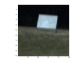
(a) August

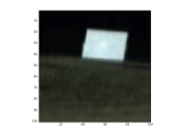
(b) September

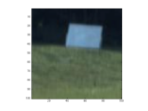
(c) October

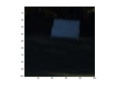
(d) November

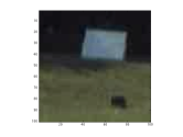
(e) October with tarp

Figure 1: Color images of the four months.

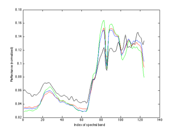
(a) Original camera spectra

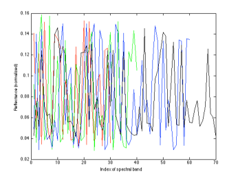
(b) Random camera spectra

Figure 2: Spectrum of a single grass pixel across the four months. Red: August, green: September, blue: October, black: November.

We set the parameter space as $\mathcal{I}=\{\text{aug, sep, oct, nov, chg}\}$, where chg denotes the October data set with the tarp in it. We also set $\mathcal{I}^{(4)}\triangleq\{\text{aug, sep, oct, nov}\}\subset\mathcal{I}$. For each $\alpha\in\mathcal{I}$, we let $X_{\alpha}$ denote the corresponding $100\times 100\times 124$ hyperspectral image. The data points $x\in X_{\alpha}$ are the spectral signatures of each pixel; that is, $|X_{\alpha}|=10000$ and $x\in\mathbb{R}^{124}$ for each $\alpha\in\mathcal{I}$. For each month as well as the changed data set, we computed a Gaussian kernel of the form:

$$k_{\alpha}(x,y)=e^{-\|x-y\|^{2}/\varepsilon(\alpha)^{2}},\quad\text{for all }\alpha\in\mathcal{I},\enspace x,y\in X_{\alpha},$$

where $\|\cdot\|$ is the Euclidean distance and $\varepsilon(\alpha)$ was selected so that the corresponding symmetric diffusion operator (matrix) $A_{\alpha}$ would have second eigenvalue $\lambda_{\alpha}^{(2)}\approx 0.97$. By forcing each diffusion operator to have approximately the same second eigenvalue, the five diffusion processes will spread at approximately the same rate. We kept the top $20$ eigenvectors and eigenvalues and computed the diffusion distance between a pixel $x$ taken from $X_{\text{chg}}$ and its corresponding pixel in $X_{\alpha}$ for each $\alpha\in\mathcal{I}^{(4)}$, i.e., we computed $D^{(t)}(x_{\text{chg}},x_{\alpha})$. The results for $t=1$ are given in Figures 3(a), 3(b), 3(c), 3(d), while the asymptotic diffusion distance as $t\rightarrow\infty$ is given in Figures 4(a), 4(b), 4(c), 4(d). We also computed the global diffusion distances between the changed data set and the four months. The results are given in Figure 5(a). Note that the diffusion distance at diffusion time $t=1$ was computed via Theorem 3.5, the asymptotic diffusion distance was computed using (17) from Remark 3.4, and the global diffusion distance was computed using Theorem 4.1.

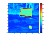
(a) August (original)

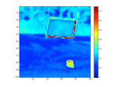
(b) September (original)

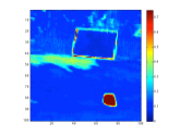
(c) October (original)

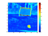
(d) November (original)

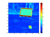
(e) August (random)

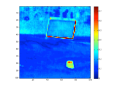
(f) September (random)

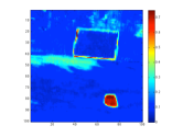
(g) October (random)

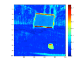
(h) November (random)

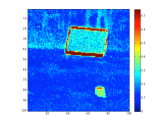
(i) August (noisy random)

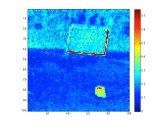
(j) September (noisy random)

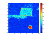
(k) October (noisy random)

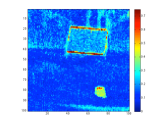
(l) November (noisy random)

Figure 3: Map of $D^{(1)}(x_{\text{chg}},x_{\alpha})$ for each $\alpha\in\mathcal{I}^{(4)}$ and for each camera type.

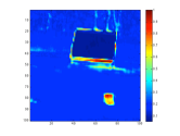
(a) August (original)

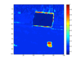
(b) September (original)

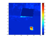
(c) October (original)

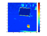
(d) November (original)

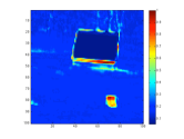
(e) August (random)

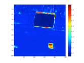
(f) September (random)

(g) October (random)

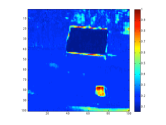
(h) November (random)

(i) August (noisy random)

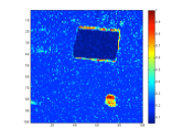
(j) September (noisy random)

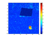
(k) October (noisy random)

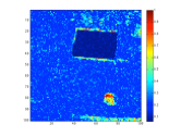
(l) November (noisy random)

Figure 4: Map of $\lim_{t\rightarrow\infty}D^{(t)}(x_{\text{chg}},x_{\alpha})$ for each $\alpha\in\mathcal{I}^{(4)}$ and for each camera type.

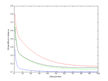
(a) Original camera

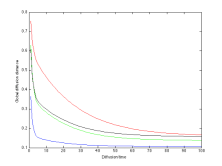
(b) Random camera

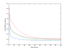
(c) Noisy random camera

Figure 5: Global diffusion distance. Red: $\mathcal{D}^{(t)}(\Gamma_{\text{chg}},\Gamma_{\text{aug}})$, green: $\mathcal{D}^{(t)}(\Gamma_{\text{chg}},\Gamma_{\text{sep}})$, blue: $\mathcal{D}^{(t)}(\Gamma_{\text{chg}},\Gamma_{\text{oct}})$, black: $\mathcal{D}^{(t)}(\Gamma_{\text{chg}},\Gamma_{\text{nov}})$

While the spectra of the various months were perturbed by the changing seasons as well as different lighting conditions, the authors of [1] did use the same camera for each image so it is reasonable to assume that one could directly compare spectra across the four months. Thus we simulated a scenario in which different cameras were used, measuring different wavelengths. In this test, a direct comparison becomes nearly impossible, and so one must turn to an indirect comparison such as the diffusion distance.

To carry out the experiment, we did the following. For each of the five images, we randomly selected $D_{\alpha}$ bands to use out of the original $124$ bands; we also randomly reordered each set of $D_{\alpha}$ bands. The values of $D_{\alpha}$ are the following: $D_{\text{aug}}=30$, $D_{\text{sep}}=40$, $D_{\text{oct}}=60$, $D_{\text{nov}}=70$, and $D_{\text{chg}}=50$. Thus for this experiment, $X_{\alpha}$, for each $\alpha\in\mathcal{I}$, contains data points in $\mathbb{R}^{D_{\alpha}}$. To see an example of these new spectra, we refer the reader to Figure 2(b). Using the measurements from this “random camera,” we then proceeded to carry out the experiment exactly as before, computing the diffusion distance for $t=1$ (Figures 3(e), 3(f), 3(g), 3(h)), the asymptotic diffusion distance (Figures 4(e), 4(f), 4(g), 4(h)), and the global diffusion distance (Figure 5(b)).

For a third and final experiment, we took the spectra from the random camera in the previous experiment and added Gaussian noise sampled from the normal distribution with mean zero and standard deviation $0.01$. This gave us an average signal to noise ratio (SNR) of $19.2$ dB (note, we compute $\text{SNR}=10\log_{10}(\text{mean}(x^{2})/\text{mean}(\eta^{2}))$, where $x$ is the signal and $\eta$ is the noise). Once more we carried out the experiment, the same as before, computing the diffusion distance for $t=1$ (Figures 3(i), 3(j), 3(k), 3(l)), the asymptotic diffusion distance (Figures 4(i), 4(j), 4(k), 4(l)), and the global diffusion distance (Figure 5(c)).

Examining Figures 3, 4, and 5, we see that the results are similar across all three cameras (the original camera, the random camera, and the noisy random camera). This result points to the two properties mentioned at the beginning of this section: that the common embedding defined by Theorem 3.5 is sensor independent and robust against noise. Thus the method is consistent under a variety of different conditions.

In terms of the change detection task, the diffusion distance is also accurate. For the diffusion time $t=1$, we see from the maps in Figure 3 that the tarp is recognized as a change. However, other changes due to the lighting or the change in seasons also appear. For example, even in October, the small change in the shadow is visible, while in August, September, and November the change in lighting causes the panel to be highlighted. Also, in some months even the trees have a weak, but noticeable difference in the their diffusion distances. When we allow $t\rightarrow\infty$ though, the smaller clusters merge together and the changes due to lighting and seasonal differences are filtered out. As one can see from Figure 4, all that is left is the change due to the added tarp (note that the change around the border of the panel is due to it being slightly shifted from month to month). Thus we see that the diffusion distance and corresponding diffusion map gives a natural representation of the data that can be used to filter types of changes at different scales. In practice, after these mappings and distances have been computed, the images can be handed off to an analyst who should be able to pick out the changes with ease; alternatively, a classification algorithm can be used on the backend (for example, one that looks for diffusion distances across images that are larger than a certain prescribed scale).

For the global diffusion distances in Figure 5, we see several intuitions borne out in this particular application. First, the closer the month in real time to October (the month in which the changed data set was recorded), the smaller the global diffusion distance. Secondly, we see that as the diffusion time $t$ gets larger, the smaller the global diffusion distance.

6.2 Parameterized difference equations

In this section we consider discrete time dynamical systems (difference equations) that depend on input parameters. The idea is to use the diffusion geometric principles outlined in this paper to understand how the geometry of the system changes as one changes the parameters of the system.

To illustrate the idea we use the following example of the Standard Map, first brought to our attention by Igor Mezić and Roy Lederman (personal correspondence). The Standard Map is an area preserving chaotic map from the torus $\mathbb{T}^{2}\triangleq 2\pi(S^{1}\times S^{1})$ onto itself. Let $(p,\theta)\in\mathbb{T}^{2}$ denote an arbitrary coordinate of the torus. For any initial condition $(p_{0},\theta_{0})\in\mathbb{T}^{2}$, the Standard Map is defined by the following two equations:

$$p_{\ell+1} \triangleq p_{\ell}+\alpha\sin(\theta_{\ell})\text{ mod }2\pi,$$

$$\theta_{\ell+1} \triangleq\theta_{\ell}+p_{\ell+1}\text{ mod }2\pi,$$

where $\alpha\in\mathcal{I}=[0,\infty)$ is a parameter, $\ell\in\mathbb{N}\cup\{0\}$, and $(p_{\ell},\theta_{\ell})\in\mathbb{T}^{2}$ for all $\ell\geq 0$. The sequence of points $\gamma(p_{0},\theta_{0})\triangleq\{(p_{\ell},\theta_{\ell})\}_{\ell\geq 0}$ constitutes the orbit derived from the initial condition $(p_{0},\theta_{0})$. When $\alpha=0$, the Standard Map consists solely of periodic and quasiperiodic orbits. For $\alpha>0$, the map is is increasingly nonlinear as $\alpha$ grows, which in turn increases the number of initial conditions that lead to chaotic dynamics.

We take the data set $X_{\alpha}$ to be the set of orbits of the Standard Map for the parameter $\alpha$. Using the ideas developed in [20, 21], it is possible to define a kernel $k_{\alpha}$ that acts on this data set. One can in turn use this kernel to define a diffusion map on the orbits. For the purposes of this experiment, we discretize the orbits by selecting a grid of initial conditions on $\mathbb{T}^{2}$ and let the system run forward a prescribed number of time steps. An example for small $\alpha$ is given in Figure 6. Notice how the diffusion map embedding into $\mathbb{R}^{3}$ organizes the Standard Map according to the geometry of the orbits.

For each $\alpha\in[0,\infty)$, we have a similar embedding. Using the ideas contained in Section 3 (in particular Theorem 3.5), it is possible to map each embedding, for all $\alpha\in\mathcal{I}$, into a single low dimensional Euclidean space. Doing so allows one to observe how the geometry of the system changes as the parameter $\alpha$ is increased; see Figure 7 for more details. In the forthcoming paper [22], we give a full treatment of these ideas.

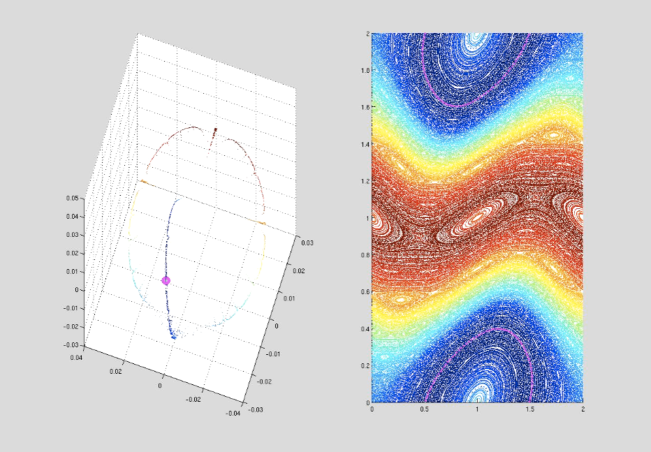
Figure 6: Diffusion map of the orbits of the Standard Map for a small $\alpha$. The color of the embedded point on the left corresponds to the orbit of the same color on the right. A particular embedded point and orbit are highlighted in purple.

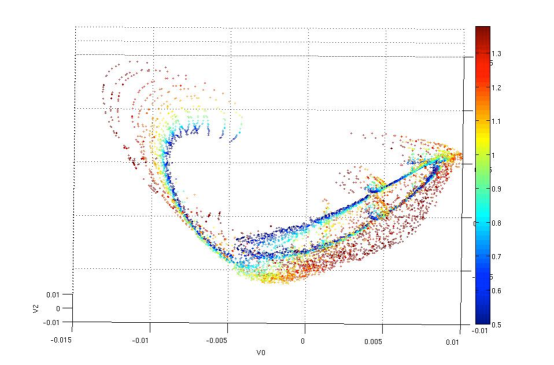
Figure 7: Common diffusion embedding of the orbits of the Standard Map across several values of $\alpha$. The color of the embedded point indicates the value of $\alpha$ used in the Standard Map. Notice, in particular, that many of the periodic and quasiperiodic orbits for low values of $\alpha$ that are embedded into the central ring of the embedding turn into chaotic orbits for higher values of $\alpha$. This in turn is realized by the diffusion map as the embedding has less structure.

6.3 Global embeddings

In this section we seek to illustrate how the global diffusion distance can be used to recover the parameters governing the global geometrical behavior of $X_{\alpha}$ as $\alpha$ ranges over $\mathcal{I}$. As an example, we shall take a torus that is being deformed according to two parameters:

1. The location of the deformation, which in this case is a pinch (imagine squeezing the torus at a certain spot).

2. The strength of the deformation, i.e., how hard we pinch the torus.

Let $\mathcal{I}=\{0,1,\ldots,30\}$. $X_{0}$ shall be the standard torus with no pinch; for $1\leq\alpha\leq 30$, $X_{\alpha}$ will have a pinch at a prescribed location on the torus with a prescribed strength. For an image of the standard torus as well as a pinched torus, see Figure 8.

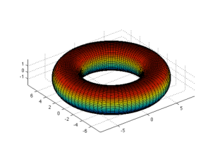
(a) Regular torus

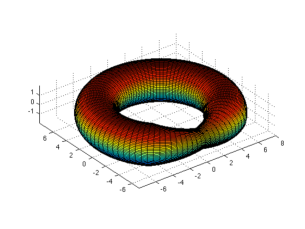
(b) Pinched torus

Figure 8: Regular and pinched torii

More specifically, we take $X_{0}$ to be a torus with a central radius of six and a lateral radius of two, i.e., $X\triangleq(6S^{1})\times(2S^{1})$. We assume that the central circle $6S^{1}$ and the lateral circle $2S^{1}$ are oriented, so that each point on the torus has a specific coordinate location (note that while $X_{0}\subset\mathbb{R}^{3}$, the points of the torus have a two dimensional coordinate system consisting of two angles, one for the central circle and one for the lateral circle).

From $X_{0}$ we build a family of “pinched” torii as follows. We pick an angle on the central circle $6S^{1}$, say $\theta_{0}$, and we pinch the torus at $\theta_{0}$ so that its lateral radius at this angle is now $r_{0}$, where $r_{0}<2$. So that we do not rip the torus, from a starting angle $\theta_{s}$, the lateral radius will decrease linearly from $2$ at $\theta_{s}$ to $r_{0}$ at $\theta_{0}$, and then increase linearly from $r_{0}$ at $\theta_{0}$ back to $2$ at some ending angle $\theta_{e}$. The lateral radius of this new torus will be $2$ at all other angles on the central circle. This is how Figure 8(b) was constructed.

We create several pinched torii as follows. We take three different angles to pinch the torus at: $\theta_{0}=\pi/2,\pi$, and $3\pi/2$. At each of these three angles, we pinch the torus so that the lateral radius $r_{0}$ at $\theta_{0}$ can take one of ten values: $r_{0}=1,1.1,1.2,\ldots,1.9$. The starting and ending angles for each pinch are offset from $\theta_{0}$ by $\pi/4$ radians, so that $\theta_{s}=\theta_{0}-\pi/4$ and $\theta_{e}=\theta_{0}+\pi/4$. Thus we have $30$ different pinched torii, which along with the original torus, gives us a family of $31$ torii.

In order to recover the two global parameters of the family of torii, we use the global diffusion distance to compute a “graph of graphs.” By this we mean the following: Let $\mathcal{G}\triangleq\{\Gamma_{\alpha}\}_{\alpha\in\mathcal{I}}$ be our family of graphs. We can compute a new graph $\Omega_{t}\triangleq(\{\Gamma_{\alpha}\}_{\alpha\in\mathcal{I}},\overline{k}_{t})$, in which $\mathcal{G}$ are the vertices of $\Omega_{t}$ and the kernel $\overline{k}_{t}:\mathcal{G}\times\mathcal{G}\rightarrow\mathbb{R}$ is a function of the global diffusion distance $\mathcal{D}^{(t)}$. One natural way to define $\overline{k}_{t}$ is via Gaussian weights:

$$\overline{k}_{t}(\Gamma_{\alpha},\Gamma_{\beta})\triangleq e^{-\mathcal{D}^{(t)}(\Gamma_{\alpha},\Gamma_{\beta})^{2}/\varepsilon^{2}},\quad\text{for all }\alpha,\beta\in\mathcal{I}.$$ (24)

Note that for each diffusion time $t$, we have a different kernel $\overline{k}_{t}$ which results in a different graph $\Omega_{t}$. Fixing a specific, but arbitrary diffusion time $t$, one can in turn construct a new diffusion operator on the graph $\Omega_{t}$ by using $\overline{k}_{t}$ as the underlying kernel. For example, if $\mathcal{I}$ is finite and we let $\overline{m}_{t}:\mathcal{G}\rightarrow\mathbb{R}$ be the density of $\overline{k}_{t}$, where

$$\overline{m}_{t}(\Gamma_{\alpha})\triangleq\sum_{\beta\in\mathcal{I}}\overline{k}_{t}(\Gamma_{\alpha},\Gamma_{\beta}),\quad\text{for all }\alpha\in\mathcal{I},$$

then the corresponding symmetric diffusion kernel $\overline{a}_{t}:\mathcal{G}\times\mathcal{G}\rightarrow\mathbb{R}$ would be defined as

$$\overline{a}_{t}(\Gamma_{\alpha},\Gamma_{\beta})\triangleq\frac{\overline{k}_{t}(\Gamma_{\alpha},\Gamma_{\beta})}{\sqrt{\overline{m}_{t}(\Gamma_{\alpha})}\sqrt{\overline{m}_{t}(\Gamma_{\beta})}},\quad\text{for all }\alpha,\beta\in\mathcal{I}.$$

Since we are assuming $\mathcal{I}$ is finite, one can think of $\overline{a}_{t}$ as an $|\mathcal{I}|\times|\mathcal{I}|$ matrix, and one can compute the eigenvectors and eigenvalues of $\overline{a}_{t}$. This gives us a diffusion map of the form

$$\overline{\Psi}_{t}^{(s)}:\mathcal{G}\rightarrow\mathbb{R}^{d},$$

where $s$ is the diffusion time for the graph of graphs. This diffusion embedding can then be used to cluster the family of graphs $\mathcal{G}$, treating each graph $\Gamma_{\alpha}\in\mathcal{G}$ as a single data point.

Our goal is to build a graph of graphs in which each vertex is one of the $31$ torii. To do so we approximate the global diffusion distance between each pair of torii by taking $7744$ random samples from $X_{0}$ (using the uniform distribution), and then using the same corresponding samples for each pinched torus. For each torus we used a Gaussian kernel of the form

$$k_{\alpha}(x,y)=e^{-\|x-y\|^{2}/\varepsilon(\alpha)^{2}},\quad\text{for all }\alpha\in\mathcal{I},$$

where $\varepsilon(\alpha)$ was selected so that the corresponding symmetric diffusion operator (matrix) $A_{\alpha}$ would have second eigenvalue $\lambda_{\alpha}^{(2)}=0.5$. The pairwise global diffusion distance was further approximated by taking the top ten eigenvalues and eigenvectors of each of the $31$ diffusion operators, and was then computed for diffusion time $t=2$ using Theorem 4.1. Two remarks: first, the diffusion time $t=2=1/(1-\lambda_{\alpha}^{(2)})$ corresponds to the approximate time it would take for the diffusion process to spread through each of the graphs; secondly, by Theorem 5.2, this approximate global diffusion distance is, with high probability, nearly equal to the true global diffusion distance between each of the torii.

After computing the pairwise global diffusion distances, we constructed the kernel $\overline{k}_{t}$, for $t=2$, defined in equation (24). We took $\varepsilon$ in this kernel to be the median of all pairwise global diffusion distances between the $31$ torii. We then computed the symmetric diffusion operator for this graph of graphs, which turned out to have second eigenvalue $\lambda^{(2)}\approx 0.48$. We took the top three eigenvalues and eigenvectors of the diffusion operator, and used them to compute the diffusion map into $\mathbb{R}^{3}$ at diffusion time $s\approx 1/(1-0.48)=1.92$.

A plot of this diffusion map is given in Figure 9. The central, dark blue, circle corresponds to the regular torus in both images. In Figure 9(a), the other three colors correspond to the angle at which the torus was pinched. In Figure 9(b), the colors correspond to the strength of the pinch (dark blue - no pinch, dark red - strongest pinch). As one can see, the diffusion embedding organizes the torii by both the location of the pinch (i.e. what arc the embedded torus lies on), and the strength of the pinch (i.e. how far from the regular torus each pinched torus lies), giving a global view of how the data set changes over the parameter space.

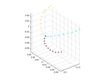
(a) Colored by location of pinch. Each color corresponds to one of the angles at which the pinch occurs.

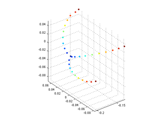
(b) Colored by strength of pinch. Dark blue indicates no pinch, followed by light blue, green, yellow, orange, and finally dark red which indicates the strongest pinch.

Figure 9: Diffusion embedding of the $31$ torii. Each data point corresponds to a torus. The embedding organizes the torii according to the two parameters governing the global geometrical behavior of the data over the parameter space.

7 Conclusion

In this paper we have generalized the diffusion distance to work on a changing graph. This new distance, along with the corresponding diffusion maps, allow one to understand how the intrinsic geometry of the data set changes over the parameter space. We have also defined a global diffusion distance between graphs, and used this to construct meta graphs in which each vertex of the meta graph corresponds to a graph. Formulas for each of these diffusion distances in terms of the spectral decompositions of the relevant diffusion operators have been proven, giving a simple and efficient way to approximate these diffusion distances. Finally, it was shown that a random, finite sample of data points from a continuous, changing data set $X$ is, with high probability, enough to approximate the diffusion distance and the global diffusion distance to high accuracy.

Future work could include generalizing these notions of diffusion distance further so that they can apply to sequences of graphs in which there is no bijective correspondence between the graphs (beyond the simple generalization of A). Also, it would be interesting to investigate how this work fits in with the recent research on vectorized diffusion operators contained in [23, 24].

8 Acknowledgements

This research was supported by Air Force Office of Scientific Research STTR FA9550-10-C-0134 and by Army Research Office MURI W911NF-09-1-0383. We would also like to thank the anonymous reviewers for their extremely helpful comments and suggestions, which greatly improved this paper.

Appendix A Non-bijective correspondence

In this appendix we consider the case in which our changing data set does not have a single bijective correspondence across the parameter set $\mathcal{I}$. We make a few small changes to the notation. Continue to let $\mathcal{I}$ denote the parameter space, but let $(\mathcal{X},\mu)$ denote a “global” measure space. Our changing data is given by $\{X_{\alpha}\}_{\alpha\in\mathcal{I}}$ with data points $x_{\alpha}\in X_{\alpha}$, and satisfies

$$X_{\alpha}\subseteq\mathcal{X},\quad\text{for all }\alpha\in\mathcal{I}.$$

We assume that each data set $X_{\alpha}$ is a measurable set under $\mu$. Suppose, additionally, that there exists a sufficiently large set $S\subset\mathcal{X}$ such that

$$S\subset X_{\alpha},\quad\text{for all }\alpha\in\mathcal{I}.$$

We maintain the remaining notations and assumptions from Section 3, and simply update them to apply for each $X_{\alpha}$. In particular, for each $\alpha\in\mathcal{I}$, we have the symmetric diffusion kernel $a_{\alpha}:X_{\alpha}\times X_{\alpha}\rightarrow\mathbb{R}$, with corresponding trace class operator $A_{\alpha}:L^{2}(X_{\alpha},\mu)\rightarrow L^{2}(X_{\alpha},\mu)$. The set of functions $\{\psi_{\alpha}^{(i)}\}_{i\geq 1}\subset L^{2}(X_{\alpha},\mu)$ still denote a set of orthonormal eigenfunctions for $A_{\alpha}$, with corresponding eigenvalues $\{\lambda_{\alpha}^{(i)}\}_{i\geq 1}$. The diffusion map is still given by $\Psi_{\alpha}^{(t)}:X_{\alpha}\rightarrow\ell^{2}$, with $\Psi_{\alpha}^{(t)}(x_{\alpha})=\left(\left(\lambda_{\alpha}^{(i)}\right)^{t}\psi_{\alpha}^{(i)}(x_{\alpha})\right)_{i\geq 1}$.

Under this more general setup, for any $\alpha,\beta\in\mathcal{I}$, the sets $X_{\alpha}\setminus X_{\beta}$ and $X_{\beta}\setminus X_{\alpha}$ may be nonempty. Thus it is not possible to compare the diffusions on $\Gamma_{\alpha}$ and $\Gamma_{\beta}$ as they spread through each graph. On the other hand, since we have a common set $S\subset X_{\alpha}\cap X_{\beta}$, we can compare the diffusion centered at $x_{\alpha}\in X_{\alpha}$ with the diffusion centered at $y_{\beta}\in X_{\beta}$ as they spread through the subgraphs of $\Gamma_{\alpha}$ and $\Gamma_{\beta}$ with common vertices $S$. Formally, we define this diffusion distance as:

$$D^{(t)}(x_{\alpha},y_{\beta};S)^{2}\triangleq\int\limits_{S}\left(a_{\alpha}^{(t)}(x_{\alpha},s)-a_{\beta}^{(t)}(y_{\beta},s)\right)^{2}\,d\mu(s),\quad\text{for all }\alpha,\beta\in\mathcal{I},\enspace(x_{\alpha},y_{\beta})\in X_{\alpha}\times X_{\beta}.$$

A result similar to Theorem 3.5 can be had for this subgraph diffusion distance. Since the eigenfunctions for $A_{\alpha}$ will not be orthonormal when restricted to $L^{2}(S,\mu)$, one must use an additional orthonormal basis $\{e^{(i)}\}_{i\geq 1}$ for $L^{2}(S,\mu)$ when rotating the diffusion maps across $\mathcal{I}$ into a common embedding. In particular, we define a new family of rotation maps $O_{\alpha,S}:\ell^{2}\rightarrow\ell^{2}$ as:

$$O_{\alpha,S}v\triangleq\left(\sum_{j\geq 1}v[j]\,\langle e^{(i)},\psi_{\alpha}^{(j)}\rangle_{L^{2}(S,\mu)}\right)_{i\geq 1}.$$

Using these rotation maps, along with the same ideas from Section 3, one can show:

$$D^{(t)}(x_{\alpha},y_{\beta};S)=\left\|O_{\alpha,S}\Psi_{\alpha}^{(t)}(x_{\alpha})-O_{\beta,S}\Psi_{\beta}^{(t)}(y_{\beta})\right\|_{\ell^{2}},\quad\text{with convergence in }L^{2}(X_{\alpha}\times X_{\beta},\mu\otimes\mu).$$

Remark A.1.

Analogously to Remark 3.6, one should be careful when choosing the basis $\{e^{(i)}\}_{i\geq 1}$ for $L^{2}(S,\mu)$. Ideally it will depend on the desired application, and can thus prioritize certain features in the data.

Appendix B Proof of random sampling theorems

In this appendix we prove the random sampling Theorems 5.1 and 5.2 from Section 5. Throughout the appendix we shall assume that $(X,\mu)$ and $\{k_{\alpha}\}_{\alpha\in\mathcal{I}}$ satisfy Assumption 2.

The proof shall rely upon a result from [17] as well as several results on the asymmetric graph Laplacian $I-P$ that are contained in [18]. All of these results are easily translated for our family of operators $\{A_{\alpha}\}_{\alpha\in\mathcal{I}}$, and we shall simply restate the needed results from [18] in these terms.

B.1 Reproducing kernel Hilbert spaces

Critical to our analysis will the be existence of a single reproducing kernel Hilbert space (RKHS) that contains the set of kernels $\{a_{\alpha}\}_{\alpha\in\mathcal{I}}$, their empirical approximations, and related functions. In [18] such a RKHS is constructed. Here we recall the definition of a RKHS as well the aforementioned construction.

A set $\mathcal{H}$ is a RKHS [25] if it is a Hilbert space of functions $f:X\rightarrow\mathbb{R}$ such that for each $x\in X$, there exists a constant $C(x)$ so that

$$f(x)\leq C(x)\,\|f\|_{\mathcal{H}}.$$

The name RKHS comes from the fact that one can show that there is a unique symmetric, positive definite kernel $h:X\times X\rightarrow\mathbb{R}$ associated with $\mathcal{H}$ such that for each $f\in\mathcal{H}$,

$$f(x)=\langle f,h(x,\cdot)\rangle_{\mathcal{H}},\quad\text{for all }x\in X.$$

We utilize a specific RKHS first presented in [18]; the construction is rewritten here for completeness. Let $l$ be a positive integer, and define the Sobolev space $\mathcal{H}^{l}$ as

$$\mathcal{H}^{l}\triangleq\{f\in L^{2}(X,dx):D^{\gamma}f\in L^{2}(X,dx)\text{ for all }|\gamma|=l\},$$

where $D^{\gamma}f$ is the weak derivative of $f$ with respect to the multi-index $\gamma\triangleq(\gamma_{1},\ldots,\gamma_{d})\in\mathbb{N}^{d}$, $|\gamma|\triangleq\gamma_{1}+\cdots+\gamma_{d}$, and $dx$ denotes the Lebesgue measure. The space $\mathcal{H}^{l}$ is a separable Hilbert space with scalar product

$$\langle f,g\rangle_{\mathcal{H}^{l}}\triangleq\langle f,g\rangle_{L^{2}(X,dx)}+\sum_{|\gamma|=l}\langle D^{\gamma}f,D^{\gamma}g\rangle_{L^{2}(X,dx)}.$$

Also note that the space $C_{b}^{l}(X)$ is a Banach space with respect to the norm

$$\|f\|_{C_{b}^{l}(X)}\triangleq\sup_{x\in X}|f(x)|+\sum_{|\gamma|=l}\sup_{x\in X}|D^{\gamma}f(x)|.$$

As explained in [18], since $X$ is bounded, we have $C_{b}^{l}(X)\subset\mathcal{H}^{l}$ and $\|f\|_{\mathcal{H}^{l}}\leq C(l)\|f\|_{C_{b}^{l}(X)}$. Via Corollary $21$ of section $4.6$ from [19], if $m\in\mathbb{N}$ and $l-m>d/2$, then we also have:

$$\mathcal{H}^{l}\subset C_{b}^{m}(X)\quad\text{and}\quad\|f\|_{C_{b}^{m}(X)}\leq C(l,m)\,\|f\|_{\mathcal{H}^{l}}.$$ (25)

Following [18], if one takes $s\triangleq\lfloor d/2\rfloor+1$, then using (25) with $l=s$ and $m=0$ we see that $\mathcal{H}^{s}$ is a RKHS with a continuous, real valued, bounded kernel $h_{s}$.

B.2 Additional operators

In this section we define several operators that will bridge the gap between the matrix $\mathbb{A}_{\alpha}$ and the operator $A_{\alpha}$. All of these definitions are based on those from [18] for the asymmetrical diffusion operators (i.e. $P$). To start, define the empirical density maps $m_{\alpha,n}:X\rightarrow\mathbb{R}$ in terms of the samples $X_{n}=\{x^{(1)},\ldots,x^{(n)}\}$ as

$$m_{\alpha,n}(x)\triangleq\frac{1}{n}\sum_{i=1}^{n}k_{\alpha}(x,x^{(i)}),\quad\text{for all }\alpha\in\mathcal{I},\enspace x\in X.$$

Note that $m_{\alpha,n}(x^{(i)})=\mathbb{D}_{\alpha}[i,i]$. We also define the empirical kernels $a_{\alpha,n}:X\times X\rightarrow\mathbb{R}$ as

$$a_{\alpha,n}(x,y)\triangleq\frac{k_{\alpha}(x,y)}{\sqrt{m_{\alpha,n}(x)}\sqrt{m_{\alpha,n}(y)}},\quad\text{for all }\alpha\in\mathcal{I},\enspace x,y\in X.$$

We then have the following lemma from [18], adapted for symmetric diffusion operators.

Lemma B.1 (Lemma $16$ from [18]).

Assume that $(X,\mu)$ and $\{k_{\alpha}\}_{\alpha\in\mathcal{I}}$ satisfy the conditions of Assumption 2. Then, for all $\alpha\in\mathcal{I}$ and for all $x\in X$,

$$k_{\alpha}(x,\cdot),m_{\alpha},m_{\alpha,n},\frac{1}{m_{\alpha}},\frac{1}{m_{\alpha,n}}\in C_{b}^{d+1}(X)\subset\mathcal{H}^{d+1}\subset\mathcal{H}^{s},$$

$$\left\|k_{\alpha}(x,\cdot)\right\|_{C_{b}^{d+1}(X)},\left\|m_{\alpha}\right\|_{C_{b}^{d+1}(X)},\left\|m_{\alpha,n}\right\|_{C_{b}^{d+1}(X)},\left\|\frac{1}{m_{\alpha}}\right\|_{C_{b}^{d+1}(X)},\left\|\frac{1}{m_{\alpha,n}}\right\|_{C_{b}^{d+1}(X)}\leq C(\alpha,d),$$

$$a_{\alpha}(x,\cdot),a_{\alpha,n}(x,\cdot)\in C_{b}^{d+1}(X)\subset\mathcal{H}^{d+1}\subset\mathcal{H}^{s},$$

$$\left\|a_{\alpha}(x,\cdot)\right\|_{\mathcal{H}^{s}},\left\|a_{\alpha,n}(x,\cdot)\right\|_{\mathcal{H}^{s}}\leq C(\alpha,d).$$

Lemma B.1 allows one to define the operators $A_{\alpha,\mathcal{H}^{s}}:\mathcal{H}^{s}\rightarrow\mathcal{H}^{s}$ and $A_{\alpha,n}:\mathcal{H}^{s}\rightarrow\mathcal{H}^{s}$,

$$(A_{\alpha,\mathcal{H}^{s}}f)(x) \triangleq\int\limits_{X}a_{\alpha}(x,y)\,\langle f,h_{s}(y,\cdot)\rangle_{\mathcal{H}^{s}}\,d\mu(y), \text{for all }\alpha\in\mathcal{I},\enspace f\in\mathcal{H}^{s},$$

$$(A_{\alpha,n}f)(x) \triangleq\frac{1}{n}\sum_{i=1}^{n}a_{\alpha,n}(x,x^{(i)})\,\langle f,h_{s}(x^{(i)},\cdot)\rangle_{\mathcal{H}^{s}}, \text{for all }\alpha\in\mathcal{I},\enspace f\in\mathcal{H}^{s}.$$

We also define similar operators $T_{\mathcal{H}^{s}}:\mathcal{H}^{s}\rightarrow\mathcal{H}^{s}$ and $T_{n}:\mathcal{H}^{s}\rightarrow\mathcal{H}^{s}$, but in terms of the reproducing kernel $h_{s}$.

$$(T_{\mathcal{H}^{s}}f)(x) \triangleq\int\limits_{X}h_{s}(x,y)\,\langle f,h_{s}(y,\cdot)\rangle_{\mathcal{H}^{s}}\,d\mu(y), \text{for all }f\in\mathcal{H}^{s},$$

$$(T_{n}f)(x) \triangleq\frac{1}{n}\sum_{i=1}^{n}h_{s}(x,x^{(i)})\,\langle f,h_{s}(x^{(i)},\cdot)\rangle_{\mathcal{H}^{s}}, \text{for all }f\in\mathcal{H}^{s}.$$

The above operators, as well as $A_{\alpha}$ and $\mathbb{A}_{\alpha}$, can be decomposed in terms of the appropriate restriction and extension operators. We begin with the two restriction operators, $R_{\mathcal{H}^{s}}:\mathcal{H}^{s}\rightarrow L^{2}(X,\mu)$ and $R_{n}:\mathcal{H}^{s}\rightarrow\mathbb{R}^{n}$.

$$(R_{\mathcal{H}^{s}}f)(x) \triangleq\langle f,h_{s}(x,\cdot)\rangle_{\mathcal{H}^{s}},\qquad\quad\enspace\text{for }\mu\text{ a.e. }x\in X,\text{ for all }f\in\mathcal{H}^{s},$$

$$R_{n}f \triangleq(f(x^{(1)}),\ldots,f(x^{(n)})),\quad\text{for all }f\in\mathcal{H}^{s}.$$

For each $\alpha\in\mathcal{I}$ we also have two extension operators, $E_{\alpha,\mathcal{H}^{s}}:L^{2}(X,\mu)\rightarrow\mathcal{H}^{s}$ and $E_{\alpha,n}:\mathbb{R}^{n}\rightarrow\mathcal{H}^{s}$, where

$$(E_{\alpha,\mathcal{H}^{s}}f)(x) \triangleq\int\limits_{X}a_{\alpha}(x,y)f(y)\,d\mu(y),\quad\text{for all }x\in X,\enspace f\in L^{2}(X,\mu),$$

$$(E_{\alpha,n}v)(x) \triangleq\frac{1}{n}\sum_{i=1}^{n}v[i]\,a_{\alpha,n}(x,x^{(i)}),\quad\text{for all }x\in X,\enspace v\in\mathbb{R}^{n}.$$

Using these operators, one can easily show the following identities:

$$A_{\alpha}=R_{\mathcal{H}^{s}}E_{\alpha,\mathcal{H}^{s}}\quad \text{and}\quad A_{\alpha,\mathcal{H}^{s}}=E_{\alpha,\mathcal{H}^{s}}R_{\mathcal{H}^{s}},$$

$$\mathbb{A}_{\alpha}=R_{n}E_{\alpha,n}\quad \text{and}\quad A_{\alpha,n}=E_{\alpha,n}R_{n},$$ (26)

$$T_{\mathcal{H}^{s}}=R_{\mathcal{H}^{s}}^{*}R_{\mathcal{H}^{s}}\quad \text{and}\quad T_{n}=R_{n}^{*}R_{n}.$$

B.3 Similarity between empirical and continuous operators

Here we collect remaining results that we shall need that involve the similarity between the empirical and continuous versions of the previously defined operators and functions. All of these results can be found in [17, 18].

Theorem B.2 ([17], also Theorem $7$ from [18]).

Suppose that $(X,\mu)$ and $\{k_{\alpha}\}_{\alpha\in\mathcal{I}}$ satisfy the conditions of Assumption 2. Let $n\in\mathbb{N}$ and sample $X_{n}=\{x^{(1)},\ldots,x^{(n)}\}\subset X$ i.i.d. according to $\mu$; also let $\tau>0$. Then the operators $T_{\mathcal{H}^{s}}$ and $T_{n}$ are Hilbert-Schmidt, and with probability $1-2e^{-\tau}$,

$$\left\|T_{\mathcal{H}^{s}}-T_{n}\right\|_{HS}\leq C(d)\frac{\sqrt{\tau}}{\sqrt{n}}.$$

Theorem B.3 (Theorem $15$ from [18]).

Suppose that $(X,\mu)$ and $\{k_{\alpha}\}_{\alpha\in\mathcal{I}}$ satisfy the conditions of Assumption 2. Let $n\in\mathbb{N}$ and sample $X_{n}=\{x^{(1)},\ldots,x^{(n)}\}\subset X$ i.i.d. according to $\mu$; also let $\tau>0$ and $\alpha\in\mathcal{I}$. Then the operators $A_{\alpha,\mathcal{H}^{s}}$ and $A_{\alpha,n}$ are Hilbert-Schmidt, and with probability $1-2e^{-\tau}$,

$$\left\|A_{\alpha,\mathcal{H}^{s}}-A_{\alpha,n}\right\|_{HS}\leq C(\alpha,d)\frac{\sqrt{\tau}}{\sqrt{n}}.$$

Lemma B.4 (Lemma $18$ from [18]).

Suppose that $(X,\mu)$ and $\{k_{\alpha}\}_{\alpha\in\mathcal{I}}$ satisfy the conditions of Assumption 2. Let $n\in\mathbb{N}$ and sample $X_{n}=\{x^{(1)},\ldots,x^{(n)}\}\subset X$ i.i.d. according to $\mu$; also let $\tau>0$ and $\alpha\in\mathcal{I}$. Then, with probability $1-2e^{-\tau}$,

$$\left\|m_{\alpha}-m_{\alpha,n}\right\|_{\mathcal{H}^{d+1}}\leq C(\alpha,d)\frac{\sqrt{\tau}}{\sqrt{n}}.$$

B.4 Proof of Theorem 5.1

In this section we prove Theorem 5.1, which we restate here.

Theorem B.5 (Theorem 5.1).

Suppose that $(X,\mu)$ and $\{k_{\alpha}\}_{\alpha\in\mathcal{I}}$ satisfy the conditions of Assumption 2. Let $n\in\mathbb{N}$ and sample $X_{n}=\{x^{(1)},\ldots,x^{(n)}\}\subset X$ i.i.d. according to $\mu$; also let $t\in\mathbb{N}$, $\tau>0$, and $\alpha,\beta\in\mathcal{I}$. Then, with probability $1-2e^{-\tau}$,

$$\left|D^{(t)}(x_{\alpha}^{(i)},x_{\beta}^{(j)})-D_{n}^{(t)}(x_{\alpha}^{(i)},x_{\beta}^{(j)})\right|\leq C(\alpha,\beta,d,t)\frac{\sqrt{\tau}}{\sqrt{n}},\quad\text{for all }i,j=1,\ldots,n.$$

Proof of Theorem 5.1.

First an additional piece of notation. Recall the $d$-dimensional index $\gamma=(\gamma_{1},\ldots,\gamma_{d})$. Let $\partial_{x}^{\gamma}a_{\alpha}$ denote the $\gamma^{\text{th}}$ partial derivative of $a_{\alpha}$ with respect to the variable $x$.

We begin with the empirical diffusion distance. Recall that $D_{n}^{(t)}(x_{\alpha}^{(i)},x_{\beta}^{(j)})^{2}=n^{2}\|\mathbb{A}_{\alpha}^{t}[i,\cdot]-\mathbb{A}_{\beta}^{t}[j,\cdot]\|_{\mathbb{R}^{n}}^{2}$. For each $i=1,\ldots,n$, define the vector $e^{(i)}\in\mathbb{R}^{n}$ as

$$e^{(i)}[j]\triangleq\left\{\begin{array}[]{ll}1,&\text{if }j=i,\\ 0,&\text{if }j\neq i,\end{array}\right.\quad\text{for all }j=1,\ldots,n.$$

We then have

$$D_{n}^{(t)}(x_{\alpha}^{(i)},y_{\beta}^{(j)})^{2} =n^{2}\left\|\mathbb{A}_{\alpha}^{t}e^{(i)}-\mathbb{A}_{\beta}^{t}e^{(j)}\right\|_{\mathbb{R}^{n}}^{2}$$

$$=n^{2}\langle\mathbb{A}_{\alpha}^{t}e^{(i)},\mathbb{A}_{\alpha}^{t}e^{(i)}\rangle_{\mathbb{R}^{n}}+n^{2}\langle\mathbb{A}_{\beta}^{t}e^{(j)},\mathbb{A}_{\beta}^{t}e^{(j)}\rangle_{\mathbb{R}^{n}}-2n^{2}\langle\mathbb{A}_{\alpha}^{t}e^{(i)},\mathbb{A}_{\beta}^{t}e^{(j)}\rangle_{\mathbb{R}^{n}}.$$ (27)

A similar expression can be had for the continuous diffusion distance. By Assumption 2, $k_{\alpha}\in C_{b}^{d+1}(X\times X)$ and $k_{\alpha}\geq C_{1}(\alpha)$. These imply that $a_{\alpha}\in C_{b}^{d+1}(X\times X)$. We can then apply Mercer’s Theorem to get that

$$a_{\alpha}^{(t)}(x,y)=\sum_{\ell\geq 1}\left(\lambda_{\alpha}^{(\ell)}\right)^{t}\psi_{\alpha}^{(\ell)}(x)\,\psi_{\alpha}^{(\ell)}(y),\quad\text{for all }(x,y)\in X\times X,$$ (28)

with absolute convergence and uniform convergence on compact subsets of $X$. In fact, since $A_{\alpha}$ is also trace class, we can get uniform convergence on all of $X$. Indeed,

$$\mathrm{Tr}(A_{\alpha})=\sum_{\ell\geq 1}\lambda_{\alpha}^{(\ell)}<\infty.$$

Therefore, for all $\varepsilon>0$ and for each $\alpha\in\mathcal{I}$, there exists $N(\varepsilon,\alpha)\in\mathbb{N}$ such that

$$\sum_{\ell>N(\varepsilon,\alpha)}\left(\lambda_{\alpha}^{(\ell)}\right)^{t}<\varepsilon.$$

Furthermore, since $a_{\alpha}$ is bounded, $\psi_{\alpha}^{(\ell)}\leq C_{2}(\alpha)$ for all $\ell\geq 1$. Therefore,

$$\sum_{\ell>N(\varepsilon,\alpha)}\left(\lambda_{\alpha}^{(\ell)}\right)^{t}\psi_{\alpha}^{(\ell)}(x)\,\psi_{\alpha}^{(\ell)}(y)\leq C_{2}(\alpha)\sum_{\ell>N(\varepsilon,\alpha)}\left(\lambda_{\alpha}^{(\ell)}\right)^{t}<C_{2}(\alpha)\,\varepsilon,\quad\text{for all }(x,y)\in X\times X.$$ (29)

Now define a family of functions $\varphi_{\alpha}^{(N,i)}\in L^{2}(X,\mu)$ for all $N\in\mathbb{N}$ and $i\in\{1,\ldots,n\}$,

$$\varphi_{\alpha}^{(N,i)}(x)\triangleq\sum_{\ell=1}^{N}\psi_{\alpha}^{(\ell)}(x^{(i)})\,\psi_{\alpha}^{(\ell)}(x).$$

We claim that

$$\left|a_{\alpha}^{(t)}(x^{(i)},x)-A_{\alpha}^{t}\varphi_{\alpha}^{(N(\varepsilon,\alpha),i)}(x)\right|<C_{2}(\alpha)\,\varepsilon,\quad\text{for all }x\in X.$$ (30)

Indeed,

$$A_{\alpha}^{t}\varphi_{\alpha}^{(N,i)}(x) =\int\limits_{X}a_{\alpha}^{(t)}(x,y)\,\varphi_{\alpha}^{(N,i)}(y)\,d\mu(y),$$

$$=\int\limits_{X}\left(\sum_{m\geq 1}\left(\lambda_{\alpha}^{(m)}\right)^{t}\psi_{\alpha}^{(m)}(x)\,\psi_{\alpha}^{(m)}(y)\right)\left(\sum_{\ell=1}^{N}\psi_{\alpha}^{(\ell)}(x^{(i)})\,\psi_{\alpha}^{(\ell)}(y)\right)\,d\mu(y),$$

$$=\sum_{m\geq 1}\sum_{\ell=1}^{N}\left(\lambda_{\alpha}^{(m)}\right)^{t}\psi_{\alpha}^{(m)}(x)\,\psi_{\alpha}^{(\ell)}(x^{(i)})\int\limits_{X}\psi_{\alpha}^{(m)}(y)\,\psi_{\alpha}^{(\ell)}(y)\,d\mu(y),$$

$$=\sum_{\ell=1}^{N}\left(\lambda_{\alpha}^{(\ell)}\right)^{t}\psi_{\alpha}^{(\ell)}(x^{(i)})\,\psi_{\alpha}^{(\ell)}(x).$$ (31)

Therefore, using (28), (31), and (29), we obtain

$$\left|a_{\alpha}^{(t)}(x^{(i)},x)-A_{\alpha}^{t}\varphi_{\alpha}^{(N(\varepsilon,\alpha),i)}(x)\right|=\left|\sum_{\ell>N(\varepsilon,\alpha)}\left(\lambda_{\alpha}^{(\ell)}\right)^{t}\psi_{\alpha}^{(\ell)}(x^{(i)})\,\psi_{\alpha}^{(\ell)}(x)\right|<C_{2}(\alpha)\,\varepsilon,$$

and so (30) holds.

Using (30), it not hard to see that

$$\left|D^{(t)}(x_{\alpha}^{(i)},y_{\beta}^{(j)})-\left\|A_{\alpha}^{t}\varphi_{\alpha}^{(N(\varepsilon,\alpha),i)}-A_{\beta}^{t}\varphi_{\beta}^{(N\varepsilon,\beta),i)}\right\|_{L^{2}(X,\mu)}\right|\leq C_{3}(\alpha,\beta)\,\varepsilon.$$

Thus it is enough to consider $\|A_{\alpha}^{t}\varphi_{\alpha}^{(N(\varepsilon,\alpha),i)}-A_{\beta}^{t}\varphi_{\beta}^{(N(\varepsilon,\beta),j)}\|_{L^{2}(X,\mu)}$. Expanding the square of this quantity one has

$$\left\|A_{\alpha}^{t}\varphi_{\alpha}^{(N(\varepsilon,\alpha),i)}-A_{\beta}^{t}\varphi_{\beta}^{(N(\varepsilon,\beta),j)}\right\|_{L^{2}(X,\mu)}^{2} =\langle A_{\alpha}^{t}\varphi_{\alpha}^{(N(\varepsilon,\alpha),i)},A_{\alpha}^{t}\varphi_{\alpha}^{(N(\varepsilon,\alpha),i)}\rangle_{L^{2}(X,\mu)}$$

$$+\langle A_{\beta}^{t}\varphi_{\beta}^{(N(\varepsilon,\beta),j)},A_{\beta}^{t}\varphi_{\beta}^{(N(\varepsilon,\beta),j)}\rangle_{L^{2}(X,\mu)}-2\langle A_{\alpha}^{t}\varphi_{\alpha}^{(N(\varepsilon,\alpha),i)},A_{\beta}^{t}\varphi_{\beta}^{(N(\varepsilon,\beta),j)}\rangle_{L^{2}(X,\mu)}.$$ (32)

The three inner products in (27) correspond to the three inner products in (32). We aim to show that each pair is nearly identical. We will do so explicitly for the pair $n^{2}\langle\mathbb{A}_{\alpha}^{t}e^{(i)},\mathbb{A}_{\beta}^{t}e^{(j)}\rangle_{\mathbb{R}^{n}}$ and $\langle A_{\alpha}^{t}\varphi_{\alpha}^{(N(\varepsilon,\alpha),i)},A_{\beta}^{t}\varphi_{\beta}^{(N(\varepsilon,\beta),j)}\rangle_{L^{2}(X,\mu)}$; the other two pairs are simply special cases of this one. We begin with the discrete inner product, for which we have the following with probability $1-2e^{-\tau}$:

$$n^{2}\langle\mathbb{A}_{\alpha}^{t}e^{(i)},\mathbb{A}_{\beta}^{t}e^{(j)}\rangle_{\mathbb{R}^{n}} =n^{2}\langle(R_{n}E_{\alpha,n})^{t}e^{(i)},(R_{n}E_{\beta,n})^{t}e^{(j)}\rangle_{\mathbb{R}^{n}}$$ (33)

$$=n^{2}\langle(E_{\alpha,n}R_{n})^{t-1}E_{\alpha,n}e^{(i)},R_{n}^{*}R_{n}(E_{\beta,n}R_{n})^{t-1}E_{\beta,n}e^{(j)}\rangle_{\mathcal{H}^{s}}$$

$$=\langle A_{\alpha,n}^{t-1}a_{\alpha,n}(x^{(i)},\cdot),T_{n}A_{\beta,n}^{t-1}a_{\beta,n}(x^{(j)},\cdot)\rangle_{\mathcal{H}^{s}}$$ (34)

$$\leq\langle A_{\alpha,\mathcal{H}^{s}}^{t-1}a_{\alpha,n}(x^{(i)},\cdot),T_{\mathcal{H}^{s}}A_{\beta,\mathcal{H}^{s}}^{t-1}a_{\beta,n}(x^{(j)},\cdot)\rangle_{\mathcal{H}^{s}}+C(\alpha,\beta,d,t)\frac{\sqrt{\tau}}{\sqrt{n}},$$ (35)

where (33) follows from (26), (34) follows from (26) and the definitions of $E_{\alpha,n}$ and $e^{(i)}$, and (35) follows from Lemma B.1, Theorem B.2, Theorem B.3, and the Cauchy-Schwarz inequality. Since the argument is symmetric, we have, with probability $1-2e^{-\tau}$,

$$\left|n^{2}\langle\mathbb{A}_{\alpha}^{t}e^{(i)},\mathbb{A}_{\beta}^{t}e^{(j)}\rangle_{\mathbb{R}^{n}}-\langle A_{\alpha,\mathcal{H}^{s}}^{t-1}a_{\alpha,n}(x^{(i)},\cdot),T_{\mathcal{H}^{s}}A_{\beta,\mathcal{H}^{s}}^{t-1}a_{\beta,n}(x^{(j)},\cdot)\rangle_{\mathcal{H}^{s}}\right|\leq C(\alpha,\beta,d,t)\frac{\sqrt{\tau}}{\sqrt{n}}.$$ (36)

Now return to the continuous inner product. With probability $1-2e^{-\tau}$, we have:

$$\langle A_{\alpha}^{t}\varphi_{\alpha}^{(N(\varepsilon,\alpha),i)},A_{\beta}^{t}\varphi_{\beta}^{(N(\varepsilon,\beta),j)}\rangle_{L^{2}(X,\mu)} =\langle(R_{\mathcal{H}^{s}}E_{\alpha,\mathcal{H}^{s}})^{t}\varphi_{\alpha}^{(N(\varepsilon,\alpha),i)},(R_{\mathcal{H}^{s}}E_{\beta,\mathcal{H}^{s}})^{t}\varphi_{\beta}^{(N(\varepsilon,\beta),j)}\rangle_{L^{2}(X,\mu)}$$ (37)

$$=\langle(E_{\alpha,\mathcal{H}^{s}}R_{\mathcal{H}^{s}})^{t-1}E_{\alpha,\mathcal{H}^{s}}\varphi_{\alpha}^{(N(\varepsilon,\alpha),i)},R_{\mathcal{H}^{s}}^{*}R_{\mathcal{H}^{s}}(E_{\beta,\mathcal{H}^{s}}R_{\mathcal{H}^{s}})^{t-1}E_{\beta,\mathcal{H}^{s}}\varphi_{\beta}^{(N(\varepsilon,\beta),j)}\rangle_{\mathcal{H}^{s}}$$

$$=\langle A_{\alpha,\mathcal{H}^{s}}^{t-1}E_{\alpha,\mathcal{H}^{s}}\varphi_{\alpha}^{(N(\varepsilon,\alpha),i)},T_{\mathcal{H}^{s}}A_{\beta,\mathcal{H}^{s}}^{t-1}E_{\beta,\mathcal{H}^{s}}\varphi_{\beta}^{(N(\varepsilon,\beta),j)}\rangle_{\mathcal{H}^{S}},$$ (38)

where (37) and (38) both follow from (26).

Examining (36) and (38), it is clear that to complete the proof we must bound the quantity $\|a_{\alpha,n}(x^{(i)},\cdot)-E_{\alpha,\mathcal{H}^{s}}\varphi_{\alpha}^{(N(\varepsilon,\alpha),i)}\|_{\mathcal{H}^{s}}$. We break it into two parts:

$$\left\|a_{\alpha,n}(x^{(i)},\cdot)-E_{\alpha,\mathcal{H}^{s}}\varphi_{\alpha}^{(N(\varepsilon,\alpha),i)}\right\|_{\mathcal{H}^{s}}\leq\left\|a_{\alpha,n}(x^{(i)},\cdot)-a_{\alpha}(x^{(i)},\cdot)\right\|_{\mathcal{H}^{s}}+\left\|a_{\alpha}(x^{(i)},\cdot)-E_{\alpha,\mathcal{H}^{s}}\varphi_{\alpha}^{(N(\varepsilon,\alpha),i)}\right\|_{\mathcal{H}^{s}}.$$ (39)

For the first part, some simple manipulations give:

$$a_{\alpha,n}(x^{(i)},x)-a_{\alpha}(x^{(i)},x)=f_{\alpha,n}^{(i)}(x)+g_{\alpha,n}^{(i)}(x),$$

where

$$f_{\alpha,n}^{(i)}(x)=\frac{k_{\alpha}(x^{(i)},x)\,(\sqrt{m_{\alpha}(x)}-\sqrt{m_{\alpha,n}(x)})}{\sqrt{m_{\alpha,n}(x^{(i)})}\sqrt{m_{\alpha,n}(x)}\sqrt{m_{\alpha}(x)}}$$

and

$$g_{\alpha,n}^{(i)}(x)=\frac{k_{\alpha}(x^{(i)},x)\,(\sqrt{m_{\alpha,n}(x^{(i)})}-\sqrt{m_{\alpha}(x^{(i)})})}{\sqrt{m_{\alpha,n}(x^{(i)})}\sqrt{m_{\alpha}(x^{(i)})}\sqrt{m_{\alpha}(x)}}.$$

For the first of these two functions, using Lemma B.1 and Lemma B.4 it is easy to see that $\|f_{\alpha,n}^{(i)}\|_{\mathcal{H}^{s}}\leq C(\alpha,d)\frac{\sqrt{\tau}}{\sqrt{n}}$ with probability $1-2e^{-\tau}$. For $g_{\alpha,n}^{(i)}$, note that

$$\left|m_{\alpha,n}(x^{(i)})-m_{\alpha}(x^{(i)})\right| \leq\sup_{x\in X}\left|m_{\alpha,n}(x)-m_{\alpha}(x)\right|$$

$$=\left\|m_{\alpha,n}-m_{\alpha}\right\|_{C_{b}^{0}(X)}$$

$$\leq C(d)\left\|m_{\alpha,n}-m_{\alpha}\right\|_{\mathcal{H}^{d+1}}$$

$$\leq C(\alpha,d)\frac{\sqrt{\tau}}{\sqrt{n}},$$ (40)

where in (40) we once again used Lemma B.4. Thus $\|g_{\alpha,n}^{(i)}\|_{\mathcal{H}^{s}}\leq C(\alpha,d)\frac{\sqrt{\tau}}{\sqrt{n}}$ with probability $1-2e^{-\tau}$, and so we have bounded the first term on the right hand side of (39). For the second term on the right hand side of (39), recall the definition of $\|\cdot\|_{\mathcal{H}^{s}}$. If we can bound $\|\partial_{x}^{\gamma}a_{\alpha}(x^{(i)},\cdot)-\partial_{x}^{\gamma}E_{\alpha,\mathcal{H}^{s}}\varphi_{\alpha}^{(N(\varepsilon,\alpha),i)}\|_{L^{2}(X,dx)}$, where $\gamma=0$ (i.e., no derivative) or $|\gamma|=s$, then we will have bounded this term as well. Note that $a_{\alpha}\in C_{b}^{d+1}(X\times X)$ implies that $\psi_{\alpha}^{(\ell)}\in C_{b}^{s}(X)$ for all $\ell\geq 1$. Furthermore, the derivative $\partial_{x}^{\gamma}a_{\alpha}(x^{(i)},\cdot)$ can be computed term by term from (28). Thus, using nearly the same argument we used to show (30), one can show that

$$\left|\partial_{x}^{\gamma}a_{\alpha}(x^{(i)},x)-\partial_{x}^{\gamma}E_{\alpha,\mathcal{H}^{s}}\varphi_{\alpha}^{(N(\varepsilon,\alpha),i)}(x)\right|<C_{4}(\alpha)\,\varepsilon,\quad\text{for all }x\in X,\enspace|\gamma|\leq s.$$ (41)

Using (41), we have:

$$\left\|\partial_{x}^{\gamma}a_{\alpha}(x^{(i)},\cdot)-\partial_{x}^{\gamma}E_{\alpha,\mathcal{H}^{s}}\varphi_{\alpha}^{(N(\varepsilon,\alpha),i)}\right\|_{L^{2}(X,dx)}\leq\sqrt{|X|}\,C_{4}(\alpha)\,\varepsilon,$$

where $|X|$ denotes the Lebesgue measure of $X$. Since $X$ was assumed to be bounded, we have $|X|\leq C$. Returning to (39), we have now shown that:

$$\left\|a_{\alpha,n}(x^{(i)},\cdot)-E_{\alpha,\mathcal{H}^{s}}\varphi_{\alpha}^{(N(\varepsilon,\alpha),i)}\right\|_{\mathcal{H}^{s}}\leq C(\alpha,d)\frac{\sqrt{\tau}}{\sqrt{n}}+C\varepsilon.$$

Taking $\varepsilon=\frac{\sqrt{\tau}}{\sqrt{n}}$ completes the proof. ∎

B.5 Proof of Theorem 5.2

Finally, we prove Theorem 5.2.

Theorem B.6 (Theorem 5.2).

Suppose that $(X,\mu)$ and $\{k_{\alpha}\}_{\alpha\in\mathcal{I}}$ satisfy the conditions of Assumption 2. Let $n\in\mathbb{N}$ and sample $X_{n}=\{x^{(1)},\ldots,x^{(n)}\}\subset X$ i.i.d. according to $\mu$; also let $t\in\mathbb{N}$, $\tau>0$, and $\alpha,\beta\in\mathcal{I}$. Then, with probability $1-2e^{-\tau}$,

$$\left|\mathcal{D}^{(t)}(\Gamma_{\alpha},\Gamma_{\beta})-\mathcal{D}^{(t)}_{n}(\Gamma_{\alpha,n},\Gamma_{\beta,n})\right|\leq C(\alpha,\beta,d,t)\frac{\sqrt{\tau}}{\sqrt{n}}.$$

Proof.

Recall that $\mathcal{D}^{(t)}(\Gamma_{\alpha},\Gamma_{\beta})=\|A_{\alpha}^{t}-A_{\beta}^{t}\|_{HS}$. From Proposition $13$ in [18], we know that $\lambda\in(0,1]$ is an eigenvalue of $A_{\alpha}$ if and only if it is an eigenvalue of $A_{\alpha,\mathcal{H}^{s}}$. Using the same ideas, one can show that $\lambda^{\prime}\neq 0$ is an eigenvalue of $A_{\alpha}^{t}-A_{\beta}^{t}$ if and only if it is an eigenvalue of $A_{\alpha,\mathcal{H}^{s}}^{t}-A_{\beta,\mathcal{H}^{s}}^{t}$. Therefore,

$$\left\|A_{\alpha}^{t}-A_{\beta}^{t}\right\|_{HS}=\left\|A_{\alpha,\mathcal{H}^{s}}^{t}-A_{\beta,\mathcal{H}^{s}}^{t}\right\|_{HS}.$$

Similarly, one can show that

$$\left\|\mathbb{A}_{\alpha}^{t}-\mathbb{A}_{\beta}^{t}\right\|_{HS}=\left\|A_{\alpha,n}^{t}-A_{\beta,n}^{t}\right\|_{HS}.$$

Thus, using the above and Theorem B.3 we have, with probability $1-2e^{-\tau}$,

$$\mathcal{D}^{(t)}(\Gamma_{\alpha},\Gamma_{\beta}) =\|A_{\alpha,\mathcal{H}^{s}}^{t}-A_{\beta,\mathcal{H}^{s}}^{t}\|_{HS}$$

$$\leq\|A_{\alpha,n}^{t}-A_{\beta,n}^{t}\|_{HS}+\|A_{\alpha,\mathcal{H}^{s}}^{t}-A_{\alpha,n}^{t}\|_{HS}+\|A_{\beta,\mathcal{H}^{s}}^{t}-A_{\beta,n}^{t}\|_{HS}$$

$$\leq\mathcal{D}^{(t)}_{n}(\Gamma_{\alpha,n},\Gamma_{\beta,n})+C(\alpha,\beta,d,t)\frac{\sqrt{\tau}}{\sqrt{n}}.$$

Since the argument is symmetric, we get the desired inequality. ∎

References

• Eismann et al. [2008] M. T. Eismann, J. Meola, R. C. Hardie, Hyperspectral change detection in the presence of diurnal and seasonal variations, IEEE Transactions on Geoscience and Remote Sensing 46 (2008) 237–249.
• Coifman and Lafon [2006] R. R. Coifman, S. Lafon, Diffusion maps, Applied and Computational Harmonic Analysis 21 (2006) 5–30.
• Vaidya et al. [2005] U. Vaidya, G. Hagen, S. Lafon, A. Banaszuk, I. Mezić, R. R. Coifman, Comparison of systems using diffusion maps, in: Proceedings of the 44th IEEE Conference on Decision and Control, and the European Control Conference 2005, Seville, Spain, pp. 7931–7936.
• Lee and Maggioni [2011] J. D. Lee, M. Maggioni, Multiscale analysis of time series of graphs, in: Proceedings of The $9^{\text{th}}$ International Conference on Sampling Theory and Applications, Singapore.
• Abdallah [2010] H. Abdallah, Processus de Diffusion sur un Flot de Variétés Riemanniennes, Ph.D. thesis, L’Universite de Grenoble, 2010.
• Mémoli [2011] F. Mémoli, A spectral notion of Gromov-Wasserstein distance and related methods, Applied and Computational Harmonic Analysis 30 (2011) 363–401.
• Roweis and Saul [2000] S. T. Roweis, L. K. Saul, Nonlinear dimensionality reduction by locally linear embedding, Science 290 (2000) 2323–2326.
• Tenenbaum et al. [2000] J. B. Tenenbaum, V. de Silva, J. C. Langford, A global geometric framework for nonlinear dimensionality reduction, Science 290 (2000) 2319–2323.
• Donoho and Grimes [2003] D. L. Donoho, C. Grimes, Hessian eigenmaps: new locally lienar embedding techniques for high-dimensional data, Proceedings of the National Academy of Sciences of the United States of America 100 (2003) 5591–5596.
• Belkin and Niyogi [2003] M. Belkin, P. Niyogi, Laplacian eigenmaps for dimensionality reduction and data representation, Neural Computation 15 (2003) 1373–1396.
• Simon [2005] B. Simon, Trace Ideals and Their Applications, volume 120 of Mathematical Surveys and Monographs, American Mathematical Society, 2nd edition, 2005.
• Coifman and Hirn [2013] R. R. Coifman, M. Hirn, Bi-stochastic kernels via asymmetric affinity functions, To appear in Applied and Computational Harmonic Analysis (2013). Also available at arXiv:1209.0237.
• Brislawn [1988] C. Brislawn, Kernels of trace class operators, Proceedings of the American Mathematical Society 104 (1988) 1181–1190.
• Brislawn [1991] C. Brislawn, Traceable integral kernels on countably generated measure spaces, Pacific Journal of Mathematics 150 (1991) 229–240.
• Mercer [1909] J. Mercer, Functions of positive and negative type and their connection with the theory of integral equations, Philosophical Transactions of the Royal Society of London, Series A 209 (1909) 415–446.
• Minh et al. [2006] H. Q. Minh, P. Niyogi, Y. Yao, Mercer’s theorem, feature maps, and smoothing, in: Conference on Learning Theory, Lecture Notes in Computer Science, Springer, Pittsburgh, Pennsylvania, USA, 2006, pp. 154–168.
• Vito et al. [2005] E. D. Vito, L. Rosasco, A. Caponnetto, U. D. Giovannini, F. Odone, Learning from examples as an inverse problem, Journal of Machine Learning Research 6 (2005) 883–904.
• Rosasco et al. [2010] L. Rosasco, M. Belkin, E. D. Vito, On learning with integral operators, Journal of Machine Learning Research 11 (2010) 905–934.
• Burenkov [1998] V. I. Burenkov, Sobolev Spaces on Domains, Teubner-Texte zur Mathematik, B.G. Teubner, Stuttgart-Leipzig, 1998.
• Levnajić and Mezić [2010] Z. Levnajić, I. Mezić, Ergodic theory and visualization I: Mesochronic plots for visualization of ergodic partition and invariant sets, Chaos 20 (2010) 033114.
• Levnajić and Mezić [2008] Z. Levnajić, I. Mezić, Ergodic theory and visualization II: Visualization of resonances and periodic sets, 2008. ArXiv:0808.2182v1.
• Coifman et al. [2012] R. R. Coifman, M. Hirn, R. Lederman, Diffusion embeddings of parameterized difference equations, 2012. In preparation.
• Singer and tieng Wu [2012] A. Singer, H. tieng Wu, Vector diffusion maps and the connection Laplacian, Communications on Pure and Applied Mathematics 65 (2012) 1067–1144.
• Wolf and Averbuch [2012] G. Wolf, A. Averbuch, Linear-projection diffusion on smooth Euclidean submanifolds, Applied and Computational Harmonic Analysis (2012). In press.
• Aronszajn [1950] N. Aronszajn, Theory of reproducing kernels, Transacations of the American Mathematical Society 68 (1950) 337–404.