Analysis of the CN and CH molecular band strengths in stars of the open cluster NGC 6791

R. Carrera Instituto de Astrofísica de Canarias, Spain Departamento de Astrofísica, Universidad de La Laguna, Spain rcarrera@iac.es

Abstract

Low resolution SDSS/SEGUE spectra have been used to study the behavior of the strengths of the CN and CH molecular bands in stars at different evolutionary stages of the open cluster NGC 6791. We find a significant spread in the strengths of the CN bands, more than twice that expected from the uncertainties, although the bimodalities observed in globular clusters are not clearly observed here. This behavior, is observed not only among red clump objects but also in unevolved stars such as those in the main sequence and lower red giant branch. In contrast, not all the stars studied show significant scatter in their CH strengths.

stars: abundances — open clusters and associations: individual: NGC 6791

1 Introduction

From the pioneering work of Osborn (1971), variations in the strength of CN molecular bands have been observed in globular cluster stars of similar luminosities at different evolutionary stages (e.g. Cannon et al., 1998; Cohen, 1999; Harbeck et al., 2003). The strength of these molecular bands depends on temperature, surface gravity, and chemical composition. Therefore, the fact that stars of similar luminosity and at the same evolutionary stage have different CN band strengths denotes a different chemical composition. These variations in CN band strength are often anti-correlated with the CH band intensity at 4300Å (e.g. Cannon et al., 1998; Harbeck et al., 2003). Moreover, detailed analyses based on high-resolution spectroscopy reveal that variations in CN strengths are accompanied by the existence of anticorrelations of the chemical abundances of other light elements (Na, O, Al, and Mg), but not for heavier elements such as Fe or Ca (Carretta et al., 2009a, b).

Several hypotheses concerning intrinsic and extrinsic factors have been proposed to explain these results (see Pancino et al., 2010b, for a recent review). However, the detection of multiple evolutionary sequences in almost all clusters properly studied (e.g. Piotto et al., 2007) indicates that the most promising one is the so-called self-enrichment scenario. First proposed by Da Costa & Cottrell (1980), this hypothesis assumes the existence of two or more subsequent stellar generations. The first stars formed pollute the gas from which the second population is formed. It seems that almost all globular clusters are massive enough to host at least two stellar populations (e.g. Carretta et al., 2010). It is therefore important to investigate what happens in less massive systems such as open clusters, which are usually younger, less massive and more metal-rich than globulars. However, studies based on open clusters using both the strength of CN bands in low-resolution spectra (Norris & Smith, 1985; Hufnagel et al., 1995; Martell & Smith, 2009) and chemical abundances derived from high-resolution spectra (de Silva et al., 2009; Smiljanic et al., 2009; Pancino et al., 2010a; Carrera & Pancino, 2011) have not found the same trends observed in globulars.

There is an intriguing stellar system, NGC 6791, with a mass intermediate between those of open and globular clusters. NGC 6791 is an ideal target for exploring the existence of chemical inhomogeneities in its stellar population. It is traditionally cataloged as an open cluster. However, its high mass ( $5\times 10^{4}$ M_⊙ Platais et al., 2011), old age ( $\sim$ 8 Gyr; e.g. Carraro et al., 2006), and high metal content ( $\sim$ +0.4 dex Carraro et al., 2006; Origlia et al., 2006; Carretta et al., 2007) differentiate this system from other open clusters. Furthermore, it is located about 1 kpc above the Galactic plane and the eccentricity of its orbit is greater than the typical value for old open clusters (Bedin et al., 2006). Previous determinations of NGC 6791’s orbit are compatible with an extragalactic origin (Carraro et al., 2006). However, proper motions derived from Hubble Space Telescope observations suggest that this cluster was formed near the Galactic bulge with a higher initial mass (Bedin et al., 2006). The total mass of NGC 6791 has decreased over time owing to repeated crossings of the denser parts of the disk. The color–magnitude diagram of NGC 6791 shows an unexpectedly wide red giant branch (RGB) and main-sequence (MS) in the region of the turn-off. Some authors have explained these features in terms of the existence of differential line-of-sight reddening (Platais et al., 2011). An alternative explanation, however, is the existence of an age spread of about 1 Gyr (Twarog et al., 2011). As well as its red clump (RC), typical of a metal-rich population, NGC 6791 also has a handful of extreme blue horizontal branch stars whose origin is still unclear (Platais et al., 2011; Buzzoni et al., 2012). Kalirai et al. (2007) associate these with strong winds due to the high-metallicity at the end of the RGB, while Bedin et al. (2008) suggest that they are the consequence of a high binary fraction. Recent investigations of globular clusters associate these extreme blue horizontal branch stars with the existence of a He-rich population (e.g. Gratton et al., 2010) although this issue remains unsolved. Janes (1984), using DDO photometry, found no signs of variations in the compositions of the RGB stars analyzed. In contrast, Hufnagel et al. (1995) found strong indications of intrinsic differences among the CN molecular band strengths in the RC stars of NGC 6791. Investigations of the composition of the stars in NGC 6791 based on high-resolution spectroscopy have found no evidence of chemical inhomogeneities (Origlia et al., 2006; Carretta et al., 2007), although an unexpected scatter in the Na abundance has been reported by Carretta et al. (2007). Geisler et al. (2012) were recently the first to report the existence of anticorrelations in the Na and O abundances in NGC 6791, similar to those observed in globular cluster stars. The goal of this paper is to investigate the behavior of the CN and CH molecular band strengths in the stars of NGC 6791 at different evolutionary stages.

This paper is organized as follows: the observational material is described in Section 2; molecular indexes are defined in Section 3; the CN and CH distributions are obtained and analyzed in Section 4; and the main results of this work are discussed and summarized in Section 5 and Section 6, respectively.

2 Observational Material

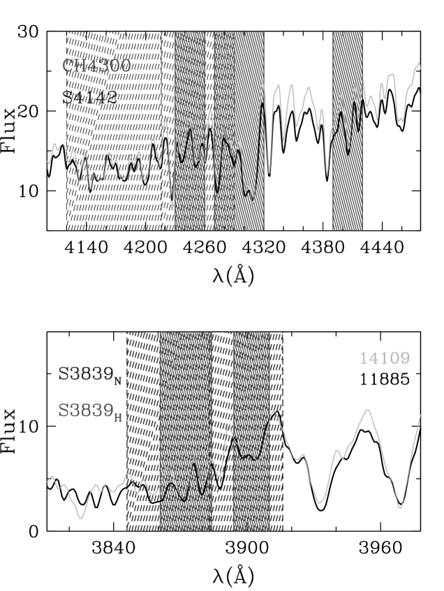
In the framework of the Sloan Extension for Galactic Understanding and Exploration (SEGUE) survey (Yanny et al., 2009), low resolution ( $R\sim 2000$ ) spectra in the wavelength range of 3600–9200Å were obtained for more than 1000 stars observed in two plates in the line of sight of NGC 6791 . They were observed to validate the SEGUE Stellar Parameter Pipeline (SSPP, Allende Prieto et al., 2008; Lee et al., 2008a, b). The reduced spectra, together with the atmosphere parameters, radial velocities, etc., derived for observed stars were made public in the eighth Sloan Digital Sky Survey (SDSS) data release (Aihara et al., 2011). The procedure for obtaining this information can be summarized as follows. Raw spectra are first reduced by the SDSS spectroscopic reduction pipeline, described in detail by Stoughton et al. (2002), which provides flux- and wavelength-calibrated spectra, together with initial determinations of the radial velocities and spectral types. More accurate radial velocities are calculated in a subsequent step by SSPP, together with determinations of metallicity, effective temperature, and surface gravity. Two examples of the spectra used in this paper are shown in Figure 1.

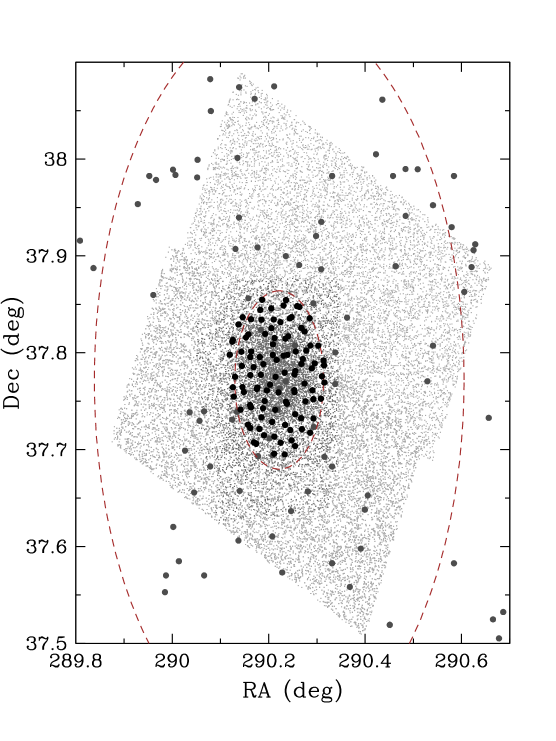
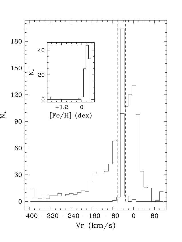
To select members of NGC 6791 from all the observed stars we followed a similar procedure as that described by Smolinski et al. (2011a). We first reject those stars located farther than 5 $\farcm$ 5¹¹1This value is $1.25\times r_{h}$ and $0.25\times r_{t}$ where $r_{h}=$ 4 $\farcm$ 4 and $r_{t}=$ 23 $\farcm$ , respectively (Platais et al., 2011). from the cluster center²²2 $\alpha_{2000}=19^{\rm h}20^{\rm m}53^{\rm s}$ $\delta_{2000}=+37\arcdeg 46\farcm 3$ (Fig. 2). This radius was chosen to ensure that stars selected were among those observed in the two photometric samples used throughout this paper and described below. We then discard those stars whose radial velocities (Fig. 3) are not within the range $\langle V_{r}\rangle_{\rm NGC\,6791}\pm 1\sigma$ , assuming $\langle V_{r}\rangle_{\rm NGC\,6791}$ =-46 $\pm$ 10 km s^-1 (Carrera et al., 2007). In the same way, we reject those stars whose metallicities (Fig. 3) do not satisfy [Fe/H] $\pm 2\sigma$ with [Fe/H] = +0.3 $\pm$ 0.15 dex (Carrera & Pancino, 2011, and references therein). A total of 104 stars were selected as NGC 6791 members according to these criteria. Although we used the same data as Smolinski et al. (2011a), our sample is bigger because we use a larger radius to select the cluster members.

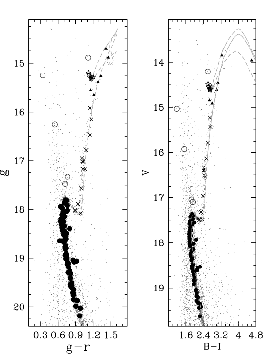
The SDSS data release also provides information about the magnitudes of the targets obtained with the SDSS photometric pipeline (Lupton et al., 2002; Tucker et al., 2006; Davenport et al., 2007). However, this pipeline was not designed to handle the high-density crowded fields typical of the central areas of clusters. Photometry from SDSS images of stellar clusters, including NGC 6791, was obtained by An et al. (2008) using the DAOPHOT/ALLFRAME packages (Stetson, 1987, 1994). The same packages have been used by Stetson et al. (2003) to derive high-quality broadband $BVI$ photometry for this cluster from 1764 CCD images. The resulting color–magnitude diagrams for NGC 6791 in each photometry system are shown in the left and right panels of Figure 4, respectively. Owing to the higher quality and lower uncertainty of the $BVI$ photometry derived by Stetson et al. (2003), we use these magnitudes in this paper. The position of stars selected in these diagrams have been used to separate them into four groups according to their evolutionary stages: 71 MS (filled circles); 14 lower RGB (lRGB, crosses); 6 upper RGB (uRGB, filled triangles); and 6 RC (open stars). Five stars were discarded because they do not fall within any of these four groups (open circles). The position of the RGB bump in an 8 Gyr old and $Z\sim 0.04$ isochrone (gray dashed line), selected from the BaSTI library (Pietrinferni et al., 2004), was used to separate stars in the lRGB and uRGB. We divided RGB stars in these two subgroups, because no pollution from material synthesized in the stellar interior is expected before the stars reach the bump. Coordinates, identification numbers, and magnitudes for selected stars are summarized in Table 1.

3 Index definition

The star-to-star light element abundance variations within globular clusters is investigated from the variations in the strength of the CN absorption bands around 3839 and 4142 Å, respectively, and the CH band around 4300 Å (e.g. Norris & Freeman, 1979; Harbeck et al., 2003; Kayser et al., 2008; Pancino et al., 2010b). The strength of each molecular band is measured with a spectral index defined as the magnitude of the difference between the integrated flux within a wavelength window containing the given feature and the integrated flux inside a nearby window, or windows, used to define the continuum. Several definitions of these indexes, used to measure the strength of each molecular band as a function of the luminosity class of the targets, can been found in the literature. This is particularly true for the 3839 CN band, where the presence of other temperature-dependent absorption lines, such as the H_ζ at 3839 Å, complicates the definition of the continuum window. Since our targets cover a wide luminosity range, we used two different indexes to measure the strength of the CN band at 3839 Å. The first one was defined by Norris et al. (1981) to sample RGB stars as:

S3839_{N}=-2.5\log\frac{F_{3846-3883}}{F_{3883-3916}}

(1)

The second one was defined by Harbeck et al. (2003) to sample properly MS objects as:

S3839_{H}=-2.5\log\frac{F_{3861-3884}}{F_{3894-3910}}

(2)

The 4142 CN band becomes useful for sampling CN variations in the case of the relatively metal-rich ([Fe/H] $\sim$ -0.7 dex) globular cluster 47 (Norris & Freeman, 1979). Pancino et al. (2010b) show that this band is less sensitive to CN variations for metal-poor MS stars. However, since NGC 6791 is much more metal-rich than globular clusters, we also studied the behavior of the the strength of this molecular band determined as (Norris & Freeman, 1979):

S4142=-2.5\log\frac{F_{4120-4216}}{F_{4216-4290}}

(3)

Finally, the G CH band at $\sim$ 4300 Å is typically used for sampling the carbon abundances in comparison with the CN bands which are used as indicators of N abundances. We measure the strength of this band using the index defined by Lee (1999):

CH4300=-2.5\log\frac{F_{4270-4320}}{0.5F_{4230-4260}+0.5F_{4390-4420}}

(4)

The adopted windows for each index have been overplotted in Figure 1. For each index, the uncertainty has been calculated as in Pancino et al. (2010b) assuming pure photon (Poisson) noise statistics in the flux measurements. The indexes and errors determined together with photometric magnitudes for each selected star are listed in Table 1. The median uncertainties for each index and evolutionary stage are listed in Table 2.

As mentioned above, two instrumental configurations were employed for the NGC 6791 region. A total of 33 stars were observed in both configurations although neither of them met the criteria used above to select NGC 6791 members. In any case, they are useful for checking the homogeneity of our data and provided an additional estimate of the uncertainties. To do this, each index was measured separately in the two spectra for each star. The medians of the differences between the values obtained for each index for all stars are: $\Delta(S3839_{N})=0.00\pm 0.02$ ; $\Delta(S3839_{H})=0.01\pm 0.02$ ; $\Delta(S4142)=0.000\pm 0.006$ ; and $\Delta(CH4300)=-0.006\pm 0.005$ . These differences are lower than the uncertainties obtained from the Poisson statistics.

Hufnagel et al. (1995) studied the CN and CH molecular band strengths in several RGB and RC stars of NGC 6791 from low resolution spectra (R $<$ 1000). Our sample has eight stars in common with that study. Although Hufnagel et al. (1995) did not use the same index definitions used here, a comparison between both sets of measures reveals systematic effects due to different instruments used in each case. The values obtained here against those determined by Hufnagel et al. (1995) for each index have been plotted in Figure 5. A clear linear correlation is observed for the CN indexes, particularly in the case of the S4142 index. This is because we used the same windows to define the continuum and band intensity as Hufnagel et al. (1995), although they obtained their indexes in a slightly different way. For each star we have calculated the difference between the value obtained here and that obtained by Hufnagel et al. (1995). We have computed the standard deviation of the differences of all stars for given indexes. The values obtained are: 0.039, 0.036, 0.010, and 0.015 for $S3839_{H}$ , $S3839_{N}$ , $S4142$ and $CH4300$ , respectively. These values are of the order of the median of the uncertainties of each index for RGB or RC stars (see Table 2).

4 CN and CH distributions

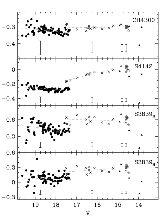
The run of the four molecular indexes defined above as a function of $V$ magnitude are shown in Figure 6. For MS stars, the strength decreases as the $V$ magnitude increases. Since temperature increases with magnitude for MS objects, the observed trend is explained by the more efficient formation of CN and CH molecules at lower temperatures. For lRGB objects, the behaviour is more random: as we ascend the RGB towards brighter magnitudes for $V\gtrsim$ 15 the indexes $S3839_{H}$ and $S4142$ increases, the index $S3839_{N}$ slightly decreases, and $CH4300$ remains almost constant. From $V\sim$ 15 a possible turnover is observed in the strengths of the indexes studied. We will come back to this point in Section 5.

4.1 Main Sequence and lower Red Giant Branch

First, we are going to focus on those stars in the MS and lRGB. As was explained above, according to stellar evolution models, it is expected that the chemical composition of their atmospheres may reflect the initial conditions of the molecular gas cloud from which the stars were formed. Before using CN and CH bands as chemical composition indicators, the temperature and gravity dependence of molecular band strengths should be removed. Different approaches can be found in the literature to removing this dependence, such as fitting the lower envelope or the median ridge line of a given molecular index as a function of color or magnitude. However, due to the low number of objects sampled in the case of the lRGB, this step should be performed with caution. To surmount this problem we adopted the following procedure. A linear least-squares fit was performed on half of the stars (randomly selected) in the lRGB. This procedure was repeated 10³ times using different random subsets each time. The final zero-point and slope for each index were obtained as the median of the zero points and slopes calculated in each individual test. The same procedure has been used for MS stars. With this procedure we tried to minimize the uncertainties due to the low number of object studied and the influence of the points on the edges. The final linear fit adopted in each case is shown as dashed lines in Figure 6 and are listed in Table 3. We calculated the corrected pseudo-indexes, denoted by a $\delta$ preceding the corresponding index, as the difference between the index and the adopted linear fit in each case.

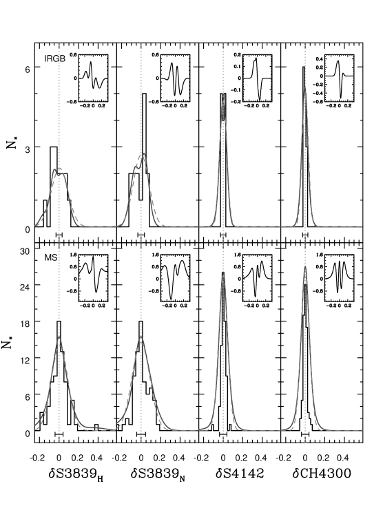
The histograms obtained for each corrected index are shown in Figure 7 for the MS (bottom) and lRGB (upper), respectively. In each case, generalized histograms (solid lines) have been derived by assuming that each star is represented by a Gaussian probability function centered on its corrected index value whose $\sigma$ is equal to the uncertainty in the determination of the index. There is no hint of bimodalities for any of the four indexes in the case of the MS. However, the distribution widths of the two S3839 indexes seem larger than that expected from the median uncertainties, as shown in the bottom of each panel, which in both cases is about 0.04 (Table 2). In fact, if we fitted each generalized histogram with a single Gaussian (dashed lines) the $\sigma$ values obtained are 0.083 $\pm$ 0.001 and 0.091 $\pm$ 0.001 for $S3839_{H}$ and $S3839_{N}$ , respectively. These values are twice as great as the uncertainties. In contrast, narrow distributions are obtained for $S4142$ and $CH4300$ . Although the median uncertainties are similar to those of S3839 indexes ( $\sim$ 0.04). In this case, the $\sigma$ obtained from the fit of a single Gaussian are 0.046 $\pm$ 0.001 and 0.045 $\pm$ 0.001, respectively. The residuals between the generalized histogram (solid lines) and the single Gaussian fitted (dashed lines) have been plotted in inset panels. They suggest that the distributions are not well reproduced by a single Gaussian.

For lRGB objects, the S4142 and CH4300 indexes, with a median uncertainty of $\sim$ 0.03, also show a narrow distribution. They are reasonably reproduced by single Gaussians (dashed lines) with $\sigma\sim$ 0.037 $\pm$ 0.001 and 0.031 $\pm$ 0.001 for $S4142$ and $CH4300$ , respectively. However, the residuals suggest that the generalized histograms have a wider dispersion than that obtained from the single Gaussian fit. In the case of two S3839 indexes a bimodality is sensed both in the normal and generalized histograms. Again, we have tried to fit each generalized distribution with a single Gaussian. In this case, the $\sigma$ values obtained are 0.086 $\pm$ 0.001 and 0.080 $\pm$ 0.001, for $S3839_{H}$ and $S3839_{N}$ , respectively. These values are almost three times the median uncertainties ( $\sim$ 0.03) in each case. Again, the residuals of the difference between the generalized histogram and the single Gaussian fit suggest that a single Gaussian does not properly reproduce the observed distributions.

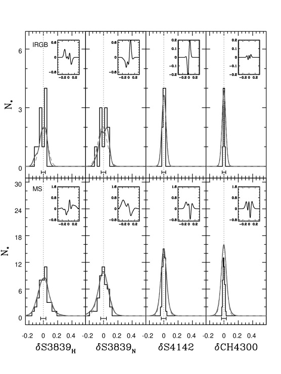
It can be argued that the wider distributions observed in the case of the $S3839$ indexes are due to our assumption of a linear dependence of the molecular band strength with temperature and gravity. This approximation may be wrong in the case of the MS turn-off and the base of the RGB. For this reason we have repeated our analysis eliminating lRGB stars fainter than V $\sim$ 17.25 mag and MS objects brighter than V $\sim$ 17.75 mag. Moreover, we have rejected MS stars fainter than V $\sim$ 18.75 mag owing to the larger uncertainties in the index determinations. The distributions of each index for the stars at each evolutionary stage are shown in Figure 8. They have been obtained following the same procedure as described previously but using the restricted samples to perform the least-squares fits in order to remove the temperature and gravity dependence. In this case, the signs of bimodalities observed in the histograms of $S3839$ indexes for lRGB stars seem clearer. However, these signs are smoothed when the generalized histograms are obtained taking into account the uncertainties. As before, the distributions are wider than those expected from the uncertainties. However, in this case the same behavior is also observed in the case of $S4142$ and $CH4300$ indexes. We have fitted each generalized histogram with a single Gaussian (dashed lines) and plotted the residuals in the inset panels. Again, the residuals suggest that the distributions are not well reproduced by a single Gaussian with the exception of the $CH4300$ index. Therefore, we conclude that the behaviors described above for each index are not influenced by the assumption of a linear dependence of the molecular index strengths with temperature and gravity for stars near the MS turn-off and in the base of the RGB. Moreover, it seems that the strengths of the $S4142$ band have the same behavior. On contrary, the CH band shows no spread.

4.2 Red Clump

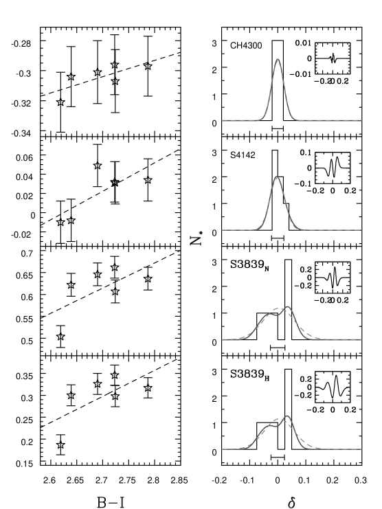
As discussed above, Hufnagel et al. (1995) studied 31 RC stars in a similar way to that described here. They found inhomogeneties of the CN bands but no signs of bimodalities as observed among globular clusters. In our sample, we have six stars in the RC region, five of them having also been studied by Hufnagel et al. (1995). In the case of RC stars, the $V$ magnitude is not useful for removing the temperature and gravity dependence since they all have similar values. For this reason, in left panels of Figure 9 each index has been plotted against the $B-I$ color. A linear fit has been performed for each index in order to remove the temperature dependence. The very small number of stars observed in the RC do not allow us to follow the same procedure used in the case of MS and lRGB stars. In each case, the corrected index has been obtained as the difference between the index and the value of the linear fit. The histograms of the distributions obtained for each corrected index have been plotted in the right panels of Figure 9. The two S3839 indexes seem to have a bimodal behavior. However, this bimodality is smoothed when the generalized histogram is obtained taking into account the uncertainties (the solid lines in the right panels of Fig. 9). In any case, the generalized histograms seem to be wider than that expected from the uncertainties. To investigate this point, we fitted a single Gaussian to each generalized histogram (dashed lines). The $\sigma$ values of the single Gaussian fitted are 0.053 $\pm$ 0.005 and 0.056 $\pm$ 0.005 for $S3839_{H}$ and $S3839_{N}$ , respectively. Therefore, the distributions obtained are twice as wide as is expected from uncertainties. A similar result was obtained by Hufnagel et al. (1995).

In the case of the S4142 and CH4300 indexes, the distributions obtained are well reproduced by a single Gaussian. Although the S4142 distributions seems slightly wider ( $\sim$ 0.03) than that expected from the uncertainties. On the contrary, the CH4300 distribution has a width ( $\sim$ 0.02) similar to the uncertainty. The lack of variations in the CH band strength for RC stars in NGC 6791 was also reported by Hufnagel et al. (1995).

5 Discussion

Significant variations and bimodalities in the strengths of the CN molecular bands, which are always anticorrelated with the CH strengths, have been widely reported in globular cluster stars at different evolutionary stages (e.g. Cannon et al., 1998; Cohen, 1999; Harbeck et al., 2003; Kayser et al., 2008; Pancino et al., 2010b; Smolinski et al., 2011b). This result is explained by the existence of different star-to-star C and N abundances. The recent discovery of several evolutionary sequences in almost all globular clusters studied (e.g. Piotto et al., 2007) has associated these chemical composition inhomogeneties with the existence of several stellar populations in each system.

In contrast, studies on open clusters, which are more metal-rich, younger, and less massive than the globulars, have not been observed similar trends (e.g. Norris & Smith, 1985; Hufnagel et al., 1995; Martell & Smith, 2009). This is interpreted in terms of open clusters being formed by a single stellar population. However, similar abundance variations to those seen among globular stars would produce smaller scatter in the CN band strengths of open cluster stars owing to their higher metallicities, with solar or above solar metal content (Hufnagel et al., 1995). Therefore, the same trends observed in globulars would be more difficult to detect in open clusters.

In this sense, NGC 6791 is a key system because it has a mass intermediate between globular and open clusters. Hufnagel et al. (1995) reported an unexpected scatter among the strengths of the CN bands in the RC stars of NGC 6791. We confirm this spread not only in evolved RC stars but also among MS and lRGB objects. Therefore, the different abundances responsible for this spread should be present in the molecular gas cloud from which NGC 6791 stars were formed. For example, the scatter observed in the strengths of CN band at 3839 Å is twice that expected from the uncertainties. Moreover, some signs of bimodalities are sensed in the distributions of the indexes used to measure the strength of this band among lRGB and RC stars. However, this result should be treated with caution owing to the the small number of stars studied in each case. We do not detect the CH–CN band strength anticorrelations observed in globular clusters, and all the stars studied seem to have a very similar CH band strength.

It is difficult to explain the CN strength dispersion observed in terms of mixing effects since this trend is also observed among unevolved stars. Moreover, Geisler et al. (2012) have recently reported an intrinsic dispersion of Na and O abundances among NGC 6791 stars in the whole RGB. These stars follow the same Na–O anticorrelation observed in globular clusters. For analogy with globular clusters, these results can be explained by the existence of multiple stellar populations, NGC 6791 being the first open cluster to show this feature. In fact,the unexpectedly wide RGB and MS observed in the NGC 6791 color–magnitude diagram indicates an age spread of about 1 Gyr (Twarog et al., 2011). However, these features could also be due to the existence of differential reddening (Platais et al., 2011).

Recent investigations have demonstrated that light element abundances are correlated with the colors of RGB stars if near ultraviolet filters (i.e. Johnson $U$ or SDSS $u$ ) are used in globular clusters (e.g. Marino et al., 2008; Milone et al., 2010, 2012; Lardo et al., 2012), although the details of this behavior are still unclear. An accurate wide-field photometric study including $U$ filter would therefore provide information about the radial distribution of the different stellar populations, which are key to investigating the process of the cluster formation and early chemical enrichment (e.g. Decressin et al., 2007; D’Ercole et al., 2008; Renzini, 2008).

Finally, the decrease in the strengths of the CN bands with magnitude for $V\lesssim 15$ needs further consideration although it is beyond the scope of this paper. A similar trend has been observed in some more metal-poor globular clusters by Smolinski et al. (2011b). This turnover may not be unusual since it has been observed by other tracers of CN band strengths, such as DDO photometry, in other open cluster; e.g. NGC 188 (McClure, 1974), NGC 2682 (Janes & Smith, 1984), and NGC 7789 (Janes, 1977). However, this question has not been studied in detail by any of these authors. A detailed study of DDO colors in stars of relatively metal-rich globular clusters shows that this decrease in CN strength is observed only for CN-rich stars and not for CN-weak objects. They compared their observations with colors obtained from synthetic spectra and concluded that, although it is expected that the mixing with material synthesized in the interior by the CN cycle should increase the N abundances, and therefore the CN strengths, the depletion of C would be so large that it would produce the decrease in the CN strengths observed, even though C is the lesser contributor to the formation of the CN molecule. In any case, a detailed analysis of this issue is necessary in order to understand the process that produces it.

6 Summary

We have studied the strengths of the CN and CH bands at 3839, 4142, and 4300 Å in stars at different evolutionary stages in the open cluster NGC 6791. This system is one of the most massive open clusters known, and according to its orbit, it should have been more massive at the time of its formation. For this analysis, we used low-resolution spectra ( $R\sim 2000$ ) obtained in the framework of the SEGUE project within the SDSS. Our main results are as follows:

•

A significant spread in the strengths of the CN molecular band at 3839 Å is observed not only in evolved red clump stars but also among objects in the main sequence and lower red giant branch. This dispersion is at least twice as great as that expected from the uncertainties. This result is obtained by the two indexes used to measure the strength of this band. This scatter is not observed in the strengths of the CN band at 4142 Å.
•

The distributions of the strengths of the two CN bands studied are not well reproduced by a single Gaussian even for main sequence stars. In fact, signs of bimodalities appear when the obtained distribution is compared with a single Gaussian.
•

No significant dispersion is observed in the strengths of the CH band at 4300 Å. In fact, the distributions of the strengths of these indexes are relatively well reproduced by a single Gaussian. This is particularly true in the case of red clump stars.
•

The strengths of the three molecular bands studied decreases as the magnitude of the star is brighter in the upper part of the red giant branch above the red clump.

I am indebted to the anonymous referee for his/her comments and suggestions which have improved significantly the analysis and the results presented in this paper. Comments on an earlier version of the manuscript by A. Aparicio, C. Gallart, M. Monelli, and N. Ospina are warmly acknowledge. R. C. acknowledges funds provided by the Spanish Ministry of Science and Innovation under the Juan de la Cierva fellowship and under the Plan Nacional de Investigación Científica, Desarrollo, e Investigación Tecnolígica, AYA2010-16717. This research has made use of the WEBDA database, operated at the Institute for Astronomy of the University of Vienna, and the SIMBAD database, operated at the CDS, Strasbourg, France Funding for SDSS-III has been provided by the Alfred P. Sloan Foundation, the Participating Institutions, the National Science Foundation, and the U.S. Department of Energy Office of Science. The SDSS-III web site is http://www.sdss3.org/. SDSS-III is managed by the Astrophysical Research Consortium for the Participating Institutions of the SDSS-III Collaboration including the University of Arizona, the Brazilian Participation Group, Brookhaven National Laboratory, University of Cambridge, University of Florida, the French Participation Group, the German Participation Group, the Instituto de Astrofisica de Canarias, the Michigan State/Notre Dame/JINA Participation Group, Johns Hopkins University, Lawrence Berkeley National Laboratory, Max Planck Institute for Astrophysics, New Mexico State University, New York University, Ohio State University, Pennsylvania State University, University of Portsmouth, Princeton University, the Spanish Participation Group, University of Tokyo, University of Utah, Vanderbilt University, University of Virginia, University of Washington, and Yale University. Facilities: SDSS(SEGUE).

References

Aihara et al. (2011) Aihara, H., Allende-Prieto, C., An, D., et al. 2011, ApJS, 193, 29
Allende Prieto et al. (2008) Allende Prieto, C., Sivarani, T., Beers, T. C., et al. 2008, AJ, 136, 2070
An et al. (2008) An, D., Johnson, J. A., Clem, J. L., et al. 2008, ApJS, 179, 326
Bedin et al. (2006) Bedin, L. R., Piotto, G., Carraro, G., King, I. R., & Anderson, J. 2006, A&A, 460, L27
Bedin et al. (2008) Bedin, L. R., Salaris, M., Piotto, G., et al. 2008, ApJ, 679, L29
Briley et al. (2001) Briley, M. M., Smith, G. H., & Claver, C. F. 2001, AJ, 122, 2561
Buzzoni et al. (2012) Buzzoni, A., Bertone, E., Carraro, G., & Buson, L. 2012, ApJ, 749, 35
Cannon et al. (1998) Cannon, R. D., Croke, B. F. W., Bell, R. A., Hesser, J. E., & Stathakis, R. A. 1998, MNRAS, 298, 601
Carrera et al. (2007) Carrera, R., Gallart, C., Pancino, E., & Zinn, R. 2007, AJ, 134, 1298
Carrera & Pancino (2011) Carrera, R., & Pancino, E. 2011, A&A, 535, 30
Carraro et al. (2006) Carraro, G., Villanova, S., Demarque, P., et al. 2006, ApJ, 643, 1151
Carretta et al. (2007) Carretta, E., Bragaglia, A., & Gratton, R. G. 2007, A&A, 473, 129
Carretta et al. (2009a) Carretta, E., Bragaglia, A., Gratton, R. G., et al. 2009a, A&A, 505, 117
Carretta et al. (2009b) Carretta, E., Bragaglia, A., Gratton, R., & Lucatello, S. 2009b, A&A, 505, 139
Carretta et al. (2010) Carretta, E., Bragaglia, A., Gratton, R. G., et al. 2010, A&A, 516, A55
Cohen (1999) Cohen, J. G. 1999, AJ, 117, 2434
Da Costa & Cottrell (1980) Da Costa, G. S., & Cottrell, P. L. 1980, ApJ, 236, L83
Davenport et al. (2007) Davenport, J. R. A., Bochanski, J. J., Covey, K. R., et al. 2007, AJ, 134, 2430
D’Ercole et al. (2008) D’Ercole, A., Vesperini, E., D’Antona, F., McMillan, S. L. W., & Recchi, S. 2008, MNRAS, 391, 825
de Silva et al. (2009) de Silva, G. M., Gibson, B. K., Lattanzio, J., & Asplund, M. 2009, A&A, 500, L25
Decressin et al. (2007) Decressin, T., Meynet, G., Charbonnel, C., Prantzos, N., & Ekström, S. 2007, A&A, 464, 1029
Geisler et al. (2012) Geisler, D., Villanova, S., Carraro, G., et al. 2012, arXiv:1207.3328
Gratton et al. (2006) Gratton, R., Bragaglia, A., Carretta, E., & Tosi, M. 2006, ApJ, 642, 462
Gratton et al. (2010) Gratton, R. G., Carretta, E., Bragaglia, A., Lucatello, S., & D’Orazi, V. 2010, A&A, 517, A81
Harbeck et al. (2003) Harbeck, D., Smith, G. H., & Grebel, E. K. 2003, AJ, 125, 197
Hufnagel et al. (1995) Hufnagel, B., Smith, G. H., & Janes, K. A. 1995, AJ, 110, 693
Janes (1984) Janes, K. A. 1984, PASP, 96, 977
Janes (1977) Janes, K. A. 1977, AJ, 82, 35
Janes & Smith (1984) Janes, K. A., & Smith, G. H. 1984, AJ, 89, 487
Kalirai et al. (2007) Kalirai, J. S., Bergeron, P., Hansen, B. M. S., et al. 2007, ApJ, 671, 748
Kayser et al. (2008) Kayser, A., Hilker, M., Grebel, E. K., & Willemsen, P. G. 2008, A&A, 486, 437
Lardo et al. (2012) Lardo, C., Milone, A. P., Marino, A. F., et al. 2012, A&A, 541, A141
Lee (1999) Lee, S.-G. 1999, AJ, 118, 920
Lee et al. (2008a) Lee, Y. S., Beers, T. C., Sivarani, T., et al. 2008a, AJ, 136, 2022
Lee et al. (2008b) Lee, Y. S., Beers, T. C., Sivarani, T., et al. 2008b, AJ, 136, 2050
Lupton et al. (2002) Lupton, R. H., Ivezic, Z., Gunn, J. E., et al. 2002, Proc. SPIE, 4836, 350
Marino et al. (2008) Marino, A. F., Villanova, S., Piotto, G., et al. 2008, A&A, 490, 625
Martell & Smith (2009) Martell, S. L., & Smith, G. H. 2009, PASP, 121, 577
McClure (1974) McClure, R. D. 1974, ApJ, 194, 355
Milone et al. (2012) Milone, A. P., Piotto, G., Bedin, L. R., et al. 2012, ApJ, 744, 58
Milone et al. (2010) Milone, A. P., Piotto, G., King, I. R., et al. 2010, ApJ, 709, 1183
Norris & Freeman (1979) Norris, J., & Freeman, K. C. 1979, ApJ, 230, L179
Norris et al. (1981) Norris, J., Cottrell, P. L., Freeman, K. C., & Da Costa, G. S. 1981, ApJ, 244, 205
Norris & Smith (1985) Norris, J., & Smith, G. H. 1985, AJ, 90, 2526
Origlia et al. (2006) Origlia, L., Valenti, E., Rich, R. M., & Ferraro, F. R. 2006, ApJ, 646, 499
Osborn (1971) Osborn, W. 1971, The Observatory, 91, 223
Pancino et al. (2010a) Pancino, E., Carrera, R., Rossetti, E., & Gallart, C. 2010a, A&A, 511, A56
Pancino et al. (2010b) Pancino, E., Rejkuba, M., Zoccali, M., & Carrera, R. 2010b, A&A, 524, A44
Pietrinferni et al. (2004) Pietrinferni, A., Cassisi, S., Salaris, M., & Castelli, F. 2004, ApJ, 612, 168
Piotto et al. (2007) Piotto, G., Bedin, L. R., Anderson, J., et al. 2007, ApJ, 661, L53
Platais et al. (2011) Platais, I., Cudworth, K. M., Kozhurina-Platais, V., et al. 2011, ApJ, 733, L1
Renzini (2008) Renzini, A. 2008, MNRAS, 391, 354
Smiljanic et al. (2009) Smiljanic, R., Gauderon, R., North, P., et al. 2009, A&A, 502, 267
Smolinski et al. (2011a) Smolinski, J. P., Lee, Y. S., Beers, T. C., et al. 2011a, AJ, 141, 89
Smolinski et al. (2011b) Smolinski, J. P., Martell, S. L., Beers, T. C., & Lee, Y. S. 2011b, AJ, 142, 126
Stetson (1987) Stetson, P. B. 1987, PASP, 99, 191
Stetson (1994) Stetson, P. B. 1994, PASP, 106, 250
Stetson et al. (2003) Stetson, P. B., Bruntt, H., & Grundahl, F. 2003, PASP, 115, 413
Stoughton et al. (2002) Stoughton, C., Lupton, R. H., Bernardi, M., et al. 2002, AJ, 123, 485
Tucker et al. (2006) Tucker, D. L., Kent, S., Richmond, M. W., et al. 2006, Astronomische Nachrichten, 327, 821
Twarog et al. (2011) Twarog, B. A., Carraro, G., & Anthony-Twarog, B. J. 2011, ApJ, 727, L7
Yanny et al. (2009) Yanny, B., Rockosi, C., Newberg, H. J., et al. 2009, AJ, 137, 4377

Refer to caption — Figure 1: Example of two CN-weak (gray line) and CN-strong (black line) spectra for two stars in the lower RGB. The IDs of these stars in the Stetson et al. (2003) reference system are 14109 and 11885, respectively. The windows used for each index have been overplotted.

Table 1: Index measurements for the sample stars.

Plate	Fiber	RA	Dec	g	g-r	ID_Stetson	V	V-I	$S3839_{H}$	$S3839_{N}$	$S4142$	$CH4300$	Region
2800	150	19:21:04.28	+37:47:18.84	14.70	1.42	11814	13.85	1.66	0.01 $\pm$ 0.02	0.33 $\pm$ 0.02	-0.07 $\pm$ 0.02	-0.30 $\pm$ 0.02	uRGB
2800	151	19:21:14.52	+37:46:32.81	17.89	0.94	14109	17.32	1.14	0.05 $\pm$ 0.04	0.51 $\pm$ 0.05	-0.15 $\pm$ 0.04	-0.32 $\pm$ 0.04	lRGB
2800	152	19:21:06.70	+37:48:08.31	18.63	0.71	12451	18.18	0.94	0.04 $\pm$ 0.07	0.29 $\pm$ 0.07	-0.26 $\pm$ 0.06	-0.32 $\pm$ 0.06	MS
2800	154	19:21:01.45	+37:48:05.11	16.47	1.14	11006	15.78	1.31	0.23 $\pm$ 0.03	0.55 $\pm$ 0.03	-0.05 $\pm$ 0.02	-0.31 $\pm$ 0.02	lRGB

Note. — Table 1 is published in its entirety in the electronic edition of the Astrophysical Journal. A portion is shown here for guidance regarding its form and content.

Table 2: Median uncertainties for each index and evolutionary stage.

Region	$S3839_{H}$	$S3839_{N}$	$S4142$	$CH4300$
MS	0.041 $\pm$ 0.002	0.045 $\pm$ 0.002	0.038 $\pm$ 0.002	0.038 $\pm$ 0.002
lRGB	0.031 $\pm$ 0.002	0.034 $\pm$ 0.003	0.028 $\pm$ 0.002	0.027 $\pm$ 0.002
uRGB	0.023 $\pm$ 0.005	0.025 $\pm$ 0.001	0.022 $\pm$ 0.003	0.021 $\pm$ 0.002
RC	0.024 $\pm$ 0.001	0.026 $\pm$ 0.001	0.022 $\pm$ 0.001	0.020 $\pm$ 0.001

Table 3: Coefficients of the linear fit used to construct the corrected pseudo-indexes and marked as dashed lines in Figs 6 and 9, respectively.

Index	Main-Sequence^a^aObtained as $index=zp+slope\times V$ .		lower Red Giant Branch^a^aObtained as $index=zp+slope\times V$ .		Red Clump^b^bObtained as $index=zp+slope\times(B-I)$ .
	zp	slope	zp	slope	zp	slope
S3839_H	0.23 $\pm$ 0.06	-0.008 $\pm$ 0.003	0.67 $\pm$ 0.20	-0.03 $\pm$ 0.01	-1.39 $\pm$ 0.25	0.59 $\pm$ 0.03
S3839_N	-0.46 $\pm$ 0.07	0.049 $\pm$ 0.004	0.42 $\pm$ 0.17	0.01 $\pm$ 0.01	-0.94 $\pm$ 0.26	0.57 $\pm$ 0.04
S4142	-0.64 $\pm$ 0.02	-0.020 $\pm$ 0.001	1.08 $\pm$ 0.06	-0.070 $\pm$ 0.004	-0.78 $\pm$ 0.03	0.296 $\pm$ 0.005
CH4300	-0.53 $\pm$ 0.01	-0.011 $\pm$ 0.001	-0.32 $\pm$ 0.04	0.001 $\pm$ 0.001	-0.597 $\pm$ 0.005	0.108 $\pm$ 0.001