The space of initial conditions and the property of an almost good reduction in discrete Painlevé II equations over finite fields

Abstract

We investigate the discrete Painlevé equations (dP${}_{\mbox{\scriptsize{II} }}$and $q$P${}_{\mbox{\scriptsize{II} }}$) over finite fields. We first show that they are well defined by extending the domain according to the theory of the space of initial conditions. Then we treat them over local fields and observe that they have a property that is similar to the good reduction of dynamical systems over finite fields. We can use this property, which can be interpreted as an arithmetic analogue of singularity confinement, to avoid the indeterminacy of the equations over finite fields and to obtain special solutions from those defined originally over fields of characteristic zero.

2000 Mathematics Subject Classification: 37K10, 34M55, 37P25

1 Introduction

In this article, we study the discrete Painlevé equations over finite fields. The discrete Painlevé equations are non-autonomous, integrable mappings which tend to some continuous Painlevé equations for appropriate choices of the continuous limit [13]. When we treate a discrete Painlevé equation over a finite field, we encounter the problem that its time evolution is not always well defined. This problem cannot be solved even if we extend the domain from ${\mathbb{F}}_{q}$ to the projective space ${\mathbb{P}}{\mathbb{F}}_{q}$, because ${\mathbb{P}}{\mathbb{F}}_{q}$ is no longer a field; we cannot determine the values such as $\frac{0}{0},\ 0\cdot\infty,\ \infty+\infty$ and so on.

There may be two strategies to define the time evolution over a finite field without inconsistencies. One is to reduce the domain so that the time evolution will not pass the indeterminate states, and the other is to extend the domain so that it can include all the orbits. We take the latter strategy and adopt two approaches.

The first approach is the application of the theory of space of initial conditions developed by Okamoto [11] and Sakai [16]. We show that the dynamics of the equations over finite fields can be well defined in the space of initial conditions.

The second approach we adopt is closely related to the theory of arithmetic dynamical systems, which concerns the dynamics over arithmetic sets such as $\mathbb{Z}$ or $\mathbb{Q}$ or a number field that is of number theoretic interest [17]. In arithmetic dynamics, the change of dynamical properties of polynomial or rational mappings give significant information when reducing them modulo prime numbers. The mapping is said to have good reduction if, roughly speaking, the reduction commutes with the mapping itself [17]. Linear fractional transformations in $\mbox{PGL}_{2}$ are typical examples of mappings with a good reduction. Recently bi-rational mappings over finite fields have been investigated in terms of integrability [15]. Since all the orbits are cyclic as far as the mapping is closed over the (projective) space of a finite field and the integrable mapping has a conserved quantity, one can estimate the distribution of orbit length by using Hesse-Weil bounds or numerical calculations. The QRT mappings [12] over finite fields have been studied in detail by choosing the parameter values so that indeterminate points are avoided [14]. They have a good reduction over finite fields.

We prove that, although most of the integrable mappings with singularities do not have a good reduction modulo a prime in general, they have an almost good reduction, which is a generalization of good reduction. We apply the method to the $q$-discrete Painlevé II equation ($q$P${}_{\mbox{\scriptsize{II} }}$). The time evolution of the discrete Painlevé equations can be well defined generically, even when not defined over the projective space of the field. In particular, the reduction from a local field ${\mathbb{Q}}_{p}$ to a finite field ${\mathbb{F}}_{p}\cup\{\infty\}$ is shown to be well defined and is used to obtain some special solutions directly from those over fields of characteristic zero such as ${\mathbb{Q}}$ or ${\mathbb{R}}$.

2 The dP${}_{\mbox{\scriptsize{II} }}$equation and its space of initial conditions

A discrete Painlevé equation is a non-autonomous and nonlinear second order ordinary difference equation with several parameters. When it is defined over a finite field, the dependent variable takes only a finite number of values and its time evolution will attain an indeterminate state in many cases for generic values of the parameters and initial conditions. For example, the dP${}_{\mbox{\scriptsize{II} }}$equation is defined as

$$u_{n+1}+u_{n-1}=\frac{z_{n}u_{n}+a}{1-u_{n}^{2}}\quad(n\in\mathbb{Z}),$$ (1)

where $z_{n}=\delta n+z_{0}$ and $a,\delta,z_{0}$ are constant parameters [10]. Let $q=p^{k}$ for a prime $p$ and a positive integer $k\in{\mathbb{Z}}_{+}$. When (1) is defined over a finite field ${\mathbb{F}}_{q}$, the dependent variable $u_{n}$ will eventually take values $\pm 1$ for generic parameters and initial values $(u_{0},u_{1})\in{\mathbb{F}}_{q}^{2}$, and we cannot proceed to evolve it. If we extend the domain from ${\mathbb{F}}_{q}^{2}$ to $({\mathbb{P}}{\mathbb{F}}_{q})^{2}=({\mathbb{F}}_{q}\cup\{\infty\})^{2}$, ${\mathbb{P}}{\mathbb{F}}_{q}$ is not a field and we cannot define arithmetic operation in (1). To determine its time evolution consistently, we have two choices: One is to restrict the parameters and the initial values to a smaller domain so that the singularities do not appear. The other is to extend the domain on which the equation is defined. In this article, we will adopt the latter approach. It is convenient to rewrite (1) as:

$$\left\{\begin{array}[]{cl}x_{n+1}&=\dfrac{\alpha_{n}}{1-x_{n}}+\dfrac{\beta_{n}}{1+x_{n}}-y_{n},\\ y_{n+1}&=x_{n},\end{array}\right.$$ (2)

where $\alpha_{n}:=\frac{1}{2}(z_{n}+a),\ \beta_{n}:=\frac{1}{2}(-z_{n}+a)$. Then we can regard (2) as a mapping defined on the domain ${\mathbb{F}}_{q}\times{\mathbb{F}}_{q}$. To resolve the indeterminacy at $x_{n}=\pm 1$, we apply the theory of the state of initial conditions developed by Sakai [16]. First we extend the domain to ${\mathbb{P}}{\mathbb{F}}_{q}\times{\mathbb{P}}{\mathbb{F}}_{q}$, and then blow it up at four points $(x,y)=(\pm 1,\infty),(\infty,\pm 1)$ to obtain the space of initial conditions:

$$\tilde{\Omega}^{(n)}:=\mathcal{A}_{(1,\infty)}^{(n)}\cup\mathcal{A}_{(-1,\infty)}^{(n)}\cup\mathcal{A}_{(\infty,1)}^{(n)}\cup\mathcal{A}_{(\infty,-1)}^{(n)},$$ (3)

where $\mathcal{A}_{(1,\infty)}^{(n)}$ is the space obtained from the two dimensional affine space ${\mathbb{A}}^{2}$ by blowing up twice as

$$\mathcal{A}_{(1,\infty)}^{(n)} :=\left\{\left((x-1,y^{-1}),[\xi_{1}:\eta_{1}],[u_{1}:v_{1}]\right)\ \Big{|}\ \right.$$

$$\qquad\eta_{1}(x-1)=\xi_{1}y^{-1},(\xi_{1}+\alpha_{n}\eta_{1})v_{1}=\eta_{1}(1-x)u_{1}\ \Big{\}}\;\subset{\mathbb{A}}^{2}\times{\mathbb{P}}\times{\mathbb{P}}.$$

Similarly,

$$\mathcal{A}_{(-1,\infty)}^{(n)} :=\left\{\left((x+1,y^{-1}),[\xi_{2}:\eta_{2}],[u_{2}:v_{2}]\right)\ \Big{|}\ \right.$$

$$\qquad\qquad\eta_{2}(x+1)=\xi_{2}y^{-1},(-\xi_{2}+\beta_{n}\eta_{2})v_{2}=\eta_{2}(1+x)u_{2}\ \Big{\}},$$

$$\mathcal{A}_{(\infty,1)}^{(n)} :=\left\{\left((x^{-1},y-1),[\xi_{3}:\eta_{3}],[u_{3}:v_{3}]\right)\ \Big{|}\ \right.$$

$$\qquad\qquad\xi_{3}(y-1)=\eta_{3}x^{-1},(\eta_{3}+\alpha_{n}\xi_{3})v_{3}=\xi_{3}(1-y)u_{3}\ \Big{\}},$$

$$\mathcal{A}_{(\infty,-1)}^{(n)} :=\left\{\left((x^{-1},y+1),[\xi_{4}:\eta_{4}],[u_{4}:v_{4}]\right)\ \Big{|}\ \right.$$

$$\qquad\qquad\xi_{4}(y+1)=\eta_{4}x^{-1},(-\eta_{4}+\beta_{n}\xi_{4})v_{3}=\xi_{4}(1+y)u_{4}\ \Big{\}}.$$

The bi-rational map (2) is extended to the bijection $\tilde{\phi}_{n}:\ \tilde{\Omega}^{(n)}\rightarrow\tilde{\Omega}^{(n+1)}$ which decomposes as $\tilde{\phi}_{n}:=\iota_{n}\circ\tilde{\omega}_{n}$. Here $\iota_{n}$ is a natural isomorphism which gives $\tilde{\Omega}^{(n)}\cong\tilde{\Omega}^{(n+1)}$, that is, on $\mathcal{A}_{(1,\infty)}^{(n)}$ for instance, $\iota_{n}$ is expressed as

$$\left((x-1,y^{-1}),[\xi:\eta],[u:v]\right)\in\mathcal{A}_{(1,\infty)}^{(n)}$$

$$\rightarrow\quad\left((x-1,y^{-1}),[\xi-\delta/2\cdot\eta:\eta],[u:v]\right)\in\mathcal{A}_{(1,\infty)}^{(n+1)}.$$

The automorphism $\tilde{\omega}_{n}$ on $\tilde{\Omega}^{(n)}$ is induced from (2) and gives the mapping

$$\mathcal{A}_{(1,\infty)}^{(n)}\rightarrow\mathcal{A}_{(\infty,1)}^{(n)},\;\mathcal{A}_{(\infty,1)}^{(n)}\rightarrow\mathcal{A}_{(-1,\infty)}^{(n)},\;\mathcal{A}_{(-1,\infty)}^{(n)}\rightarrow\mathcal{A}_{(\infty,-1)}^{(n)},\;\mathcal{A}_{(\infty,-1)}^{(n)}\rightarrow\mathcal{A}_{(1,\infty)}^{(n)}.$$

Under the map $\mathcal{A}_{(1,\infty)}^{(n)}\rightarrow\mathcal{A}_{(\infty,1)}^{(n)}$,

$$x=1\ \rightarrow\ E_{2}^{(\infty,1)} \qquad u_{3}=\left(y-\frac{\beta_{n}}{2}\right)v_{3},$$

$$E_{1}^{(1,\infty)}\ \rightarrow\ E_{1}^{(\infty,1)} \qquad[\xi_{1}:-\eta_{1}]=[\alpha_{n}\xi_{3}+\eta_{3}:\xi_{3}],$$

$$E_{2}^{(1,\infty)}\ \rightarrow\ y^{\prime}=1 \qquad x^{\prime}=\frac{u_{1}}{v_{1}}+\frac{\beta_{n}}{2},$$

where $(x,y)\in\mathcal{A}_{(1,\infty)}^{(n)}$, $(x^{\prime},y^{\prime})\in\mathcal{A}_{(\infty,1)}^{(n)}$, $E_{1}^{\mbox{\scriptsize p}}$ and $E_{2}^{\mbox{\scriptsize p}}$ are the exceptional curves in $\mathcal{A}_{\mbox{\scriptsize p}}^{(n)}$ obtained by the first blowing up and the second blowing up respectively at the point p $\in\{(\pm 1,\infty),(\infty,\pm 1)\}$. Similarly under the map $\mathcal{A}_{(\infty,1)}^{(n)}\rightarrow\mathcal{A}_{(-1,\infty)}^{(n)}$,

$$E_{1}^{(\infty,1)}\ \rightarrow\ E_{1}^{(-1,\infty)} \qquad[\xi_{3}:\eta_{3}]=[\eta_{2}:(\beta_{n}-\alpha_{n})\eta_{2}-\xi_{2}],$$

$$E_{2}^{(\infty,1)}\ \rightarrow\ E_{2}^{(-1,\infty)} \qquad[u_{3}:v_{3}]=[-\beta_{n}u_{2}:\alpha_{n}v_{2}].$$

The mapping on the other points are defined in a similar manner. Note that $\tilde{\omega}_{n}$ is well-defined in the case $\alpha_{n}=0$ or $\beta_{n}=0$. In fact, for $\alpha_{n}=0$, $E_{2}^{(1,\infty)}$ and $E_{2}^{(\infty,1)}$ can be identified with the lines $x=1$ and $y=1$ respectively. Therefore we have found that, through the construction of the space of initial conditions, the dP${}_{\mbox{\scriptsize{II} }}$equation can be well-defined over finite fields. However there are some unnecessary elements in the space of initial conditions when we consider a finite field, because we are working on a discrete topology and do not need continuity of the map. Let $\tilde{\Omega}^{(n)}$ be the space of initial conditions and $|\tilde{\Omega}^{(n)}|$ be the number of elements of it. For the dP${}_{\mbox{\scriptsize{II} }}$equation, we obtain $|\tilde{\Omega}^{(n)}|=(q+1)^{2}-4+4(q+1)-4+4(q+1)=q^{2}+10q+1$, since ${\mathbb{P}}{\mathbb{F}}_{q}$ contains $q+1$ elements. However an exceptional curve $E_{1}^{\mbox{\scriptsize p}}$ is transferred to another exceptional curve $E_{1}^{\mbox{\scriptsize p}^{\prime}}$, and $[1:0]\in E_{2}^{\mbox{\scriptsize p}}$ to $[1:0]\in E_{2}^{\mbox{\scriptsize p}^{\prime}}$ or to a point in $E_{1}^{\mbox{\scriptsize p}^{\prime}}$. Hence we can reduce the space of initial conditions $\tilde{\Omega}^{(n)}$ to the minimal space of initial conditions $\Omega^{(n)}$ which is the minimal subset of $\tilde{\Omega}^{(n)}$ including ${\mathbb{P}}{\mathbb{F}}_{q}\times{\mathbb{P}}{\mathbb{F}}_{q}$, closed under the time evolution. By subtracting unnecessary elements we find $|\Omega^{(n)}|=(q+1)^{2}-4+4(q+1)-4=q^{2}+6q-3$. In summary, we obtain the following proposition:

Theorem 2.1.

The domain of the dP${}_{\mbox{\scriptsize{II} }}$equation over ${\mathbb{F}}_{q}$ can be extended to the minimal domain $\Omega^{(n)}$ on which the time evolution at time step $n$ is well defined. Moreover $|\Omega^{(n)}|=q^{2}+6q-3$.

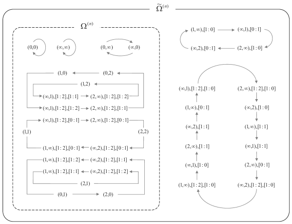
Figure 1: The orbit decomposition of the space of initial conditions $\tilde{\Omega}^{(n)}$ and the reduced one $\Omega^{(n)}$ for $q=3$.

In figure 1, we show a schematic diagram of the map $\tilde{\omega}_{n}$ on $\tilde{\Omega}^{(n)}$, and its restriction map $\omega_{n}:=\tilde{\omega}_{n}|_{\Omega^{(n)}}$ on $\Omega^{(n)}$ with $q=3$, $\alpha_{0}=1$ and $\beta_{0}=2$. We can also say that the figure 1 is a diagram for the autonomous version of the equation (2) when $\delta=0$. In the case of $q=3$, we have $|\tilde{\Omega}^{(n)}|=40$ and $|\Omega^{(n)}|=24$.

The above approach is equally valid for the other discrete Painlevé equations and we can define them over finite fields by constructing isomorphisms on the spaces of initial conditions. Thus we conclude that a discrete Painlevé equation can be well defined over a finite field by redefining the initial domain properly. However, for a general nonlinear equation, explicit construction of the space of initial conditions over a finite field is not so straightforward [18] and it will not help us to obtain the explicit solutions. In the next section, we show another extention of the space of initial conditions: we extend it to ${\mathbb{Z}}_{p}\times{\mathbb{Z}}_{p}$.

3 The $q$P${}_{\mbox{\scriptsize{II} }}$equation over a local field and its reduction modulo a prime

Let $p$ be a prime number and for each $x\in{\mathbb{Q}}$ ($x\neq 0$) write $x=p^{v_{p}(x)}\dfrac{u}{v}$ where $v_{p}(x),u,v\in{\mathbb{Z}}$ and $u$ and $v$ are coprime integers neither of which is divisible by $p$. The $p$-adic norm $|x|_{p}$ is defined as $|x|_{p}=p^{-v_{p}(x)}$. ($|0|_{p}=0$.) The local field ${\mathbb{Q}}_{p}$ is a completion of ${\mathbb{Q}}$ with respect to the $p$-adic norm. It is called the field of $p$-adic numbers and its subring ${\mathbb{Z}}_{p}:=\{x\in{\mathbb{Q}}_{p}|\ |x|_{p}\leq 1\}$ is called the ring of $p$-adic integers [9]. The $p$-adic norm satisfies a non-archimedean (ultrametric) triangle inequality $|x+y|_{p}\leq\max[|x|_{p},|y|_{p}]$. Let $\mathfrak{p}=p{\mathbb{Z}}_{p}=\left\{x\in{\mathbb{Z}}_{p}|\ v_{p}(x)\geq 1\right\}$ be the maximal ideal of ${\mathbb{Z}}_{p}$. We define the reduction of $x$ modulo $\mathfrak{p}$ as $\tilde{x}$: ${\mathbb{Z}}_{p}\ni x\mapsto\tilde{x}\in{\mathbb{Z}}_{p}/\mathfrak{p}\cong{\mathbb{F}}_{p}$. Note that the reduction is a ring homomorphism. The reduction is generalized to ${\mathbb{Q}}_{p}^{\times}$:

$${\mathbb{Q}}_{p}^{\times}\ni x=p^{k}u\ (u\in{\mathbb{Z}}_{p}^{\times})\mapsto\left\{\begin{array}[]{cl}0&(k>0)\\ \infty&(k<0)\\ \tilde{u}&(k=0)\end{array}\right.\in{\mathbb{P}}{\mathbb{F}}_{p},$$

which is no longer homomorphic. For a rational map of the plane

$$\phi(x,y)=(\phi_{1}(x,y),\phi_{2}(x,y))\in(\mathbb{Z}_{p}(x,y))^{2}:\ \mathcal{D}\subseteq{\mathbb{Z}}_{p}^{2}\to{\mathbb{Z}}_{p}^{2},$$

defined on some domain $\mathcal{D}$,

$$\tilde{\phi}(x,y)=(\tilde{\phi}_{1}(x,y),\tilde{\phi}_{2}(x,y))\in(\mathbb{F}_{p}(x,y))^{2}$$

is defined as the map whose coefficients are all reduced. The rational system $\phi$ is said to have a good reduction (modulo $\mathfrak{p}$ on the domain $\mathcal{D}$) if we have $\widetilde{\phi(x,y)}=\tilde{\phi}(\tilde{x},\tilde{y})$ for any $(x,y)\in\mathcal{D}$ [17]. We have defined a generalized notion in our previous letter and have explained its usefulness;

Definition 3.1 ([6]).

A (non-autonomous) rational system $\phi_{n}$: ${\mathbb{Q}}_{p}^{2}\to{\mathbb{Q}}_{p}^{2}$ $(n\in{\mathbb{Z}})$ is said to have an almost good reduction modulo $\mathfrak{p}$ on the domain $\mathcal{D}\subseteq{\mathbb{Z}}_{p}^{2}$, if there exists a positive integer $m_{\mbox{\rm\scriptsize p};n}$ for any $\mbox{\rm p}=(x,y)\in\mathcal{D}$ and time step $n$ such that

$$\widetilde{\phi_{n}^{m_{\mbox{\rm\tiny p};n}}(x,y)}=\widetilde{\phi_{n}^{m_{\mbox{\rm\tiny p};n}}}(\tilde{x},\tilde{y}),$$ (4)

where $\phi_{n}^{m}:=\phi_{n+m-1}\circ\phi_{n+m-2}\circ\cdots\circ\phi_{n}$.

If we can take $m_{\mbox{\rm\scriptsize p};n}=1$, then the mapping has a good reduction. Let us first review some of the previous findings in order to see the significance of the notion of almost good reduction. Let us consider the mapping $\Psi_{\gamma}$:

$$\left\{\begin{array}[]{cl}x_{n+1}&=\dfrac{x_{n}+1}{x_{n}^{\gamma}y_{n}}\\ y_{n+1}&=x_{n}\end{array}\right.,$$ (5)

where $\gamma\in{\mathbb{Z}}_{\geq 0}$ is a non-negative integer parameter. The map (5) is known to be integrable if and only if $\gamma=0,1,2$. When $\gamma=0,1,2$, the map (5) belongs to the QRT family and is integrable in the sense that it has a conserved quantity. We also note that the system (5) can be seen as an autonomous version of the $q$-discrete Painlevé I equation for $\gamma=0,1,2$. We have proved that, in this example, the integrability is equivalent to having almost good reduction.

Proposition 3.2 ([6]).

The rational mapping (5) has an almost good reduction modulo $\mathfrak{p}$ on the domain $\mathcal{D}=\{(x,y)\in{\mathbb{Z}}_{p}^{2}\ |x\neq 0,y\neq 0\}$, if and only if $\gamma=0,1,2$.

In the previous work, the dP${}_{\mbox{\scriptsize{II} }}$equation, too, has been proved to have almost good reduction. It is reasonable to postulate that almost good reduction is closely related to the integrability of maps of the plane. We further clarify this point by demonstrating that $q$-discrete analogue of the Painlevé II equation also has almost good reduction. The $q$-discrete analogue of Painlevé II equation ($q$P${}_{\mbox{\scriptsize{II} }}$equation) is a following $q$-difference equation:

$$(z(q\tau)z(\tau)+1)(z(\tau)z(q^{-1}\tau)+1)=\frac{a\tau^{2}z(\tau)}{\tau-z(\tau)},$$ (6)

where $a$ and $q$ are parameters [4]. It is also convenient to rewrite (6) as a system form

$$\Phi_{n}:\left\{\begin{array}[]{cl}x_{n+1}&=\dfrac{a(q^{n}\tau_{0})^{2}x_{n}-(q^{n}\tau_{0}-x_{n})(1+x_{n}y_{n})}{x_{n}(q^{n}\tau_{0}-x_{n})(x_{n}y_{n}+1)},\\ y_{n+1}&=x_{n},\end{array}\right.$$ (7)

where $\tau=q^{n}\tau_{0}$. We can prove the following proposition:

Proposition 3.3.

Suppose that $a,q,\tau_{0}$ are integers not divisible by $p$, then the mapping (7) has an almost good reduction modulo $\mathfrak{p}$ on the domain $\mathcal{D}:=\{(x,y)\in{\mathbb{Z}}_{p}^{2}\ |x\neq 0,x\neq q^{n}\tau_{0}\ (n\in{\mathbb{Z}}),xy+1\neq 0\}$.

Proof 3.4.

Let $(x_{n+1},y_{n+1})=\Phi_{n}(x_{n},y_{n})$. We only examine the cases $\tilde{x}_{n}=0$ or $\widetilde{q^{n}\tau_{0}}$ or $-\tilde{y}_{n}^{-1}$. (It is due to the fact that the mapping trivially has good reduction for other points $(x_{n},y_{n})$.) We use the abbreviation $\tilde{q}=q,\tilde{\tau}=\tau,\tilde{a}=a$ for simplicity. By direct computation, we obtain;
(i) If $\tilde{x}_{n}=0$ and $-1+q^{2}-aq^{2}\tau^{2}+q^{3}\tau^{2}-q^{2}\tau\tilde{y}_{n}\neq 0$,

$$\widetilde{\Phi_{n}^{3}(x_{n},y_{n})}=\widetilde{\Phi_{n}^{3}}(\tilde{x}_{n}=0,\tilde{y}_{n})=\left(\frac{1-q^{2}+aq^{2}\tau^{2}-q^{3}\tau^{2}-aq^{4}\tau^{2}+q^{2}\tau\tilde{y}_{n}}{q^{2}\tau(-1+q^{2}-aq^{2}\tau^{2}+q^{3}\tau^{2}-q^{2}\tau\tilde{y}_{n})},q^{2}\tau\right).$$

(ii) If $\tilde{x}_{n}=0$ and $-1+q^{2}-aq^{2}\tau^{2}+q^{3}\tau^{2}-q^{2}\tau\tilde{y}_{n}=0$,

$$\widetilde{\Phi_{n}^{5}(x_{n},y_{n})}=\widetilde{\Phi_{n}^{5}}(\tilde{x}_{n}=0,\tilde{y}_{n})=\left(\frac{1-q^{2}+q^{7}\tau^{2}-aq^{8}\tau^{2}}{q^{4}\tau},0\right).$$

(iii) If $\tilde{x}_{n}=\tau$ and $1+\tau\tilde{y}_{n}\neq 0$,

$$\widetilde{\Phi_{n}^{3}(x_{n},y_{n})}=\widetilde{\Phi_{n}^{3}}(\tilde{x}_{n}=\tau,\tilde{y}_{n})$$

$$\quad=\left(\frac{1-q^{2}+(a+q-aq^{2})q^{2}\tau^{2}+(1-q^{2})\tau\tilde{y}+(1-aq)q^{3}\tau^{3}\tilde{y}}{q^{2}\tau(1+\tau\tilde{y}_{n})},0\right).$$

(iv) If $\tilde{x}_{n}=\tau$ and $1+\tau\tilde{y}_{n}=0$,

$$\widetilde{\Phi_{n}^{7}(x_{n},y_{n})}=\widetilde{\Phi_{n}^{7}}(\tilde{x}_{n}=\tau,\tilde{y}_{n})=\left(\frac{1}{aq^{12}\tau^{3}},-aq^{12}\tau^{3}\right).$$

(v) If $\tilde{x}_{n}\tilde{y}_{n}+1=0$,

$$\widetilde{\Phi_{n}^{7}(x_{n},y_{n})}=\widetilde{\Phi_{n}^{7}}(\tilde{x}_{n}=-\tilde{y}_{n}^{-1},\tilde{y}_{n})=\left(-\frac{1}{aq^{12}\tau^{4}\tilde{y}_{n}},aq^{12}\tau^{4}\tilde{y}_{n}\right).$$

Thus we complete the proof.

From this proposition we can explicitly define the time evolution of the $q$P${}_{\mbox{\scriptsize{II} }}$equation. We can also consider the special solutions for qP${}_{\mbox{\scriptsize{II} }}$equation (6) over ${\mathbb{P}}{\mathbb{F}}_{p}$. In [3] it has been proved that (6) over ${\mathbb{C}}$ with $a=q^{2N+1}$ $(N\in{\mathbb{Z}})$ is solved by the functions given by

$$z^{(N)}(\tau) =\begin{cases}\displaystyle\frac{g^{(N)}(\tau)g^{(N+1)}(q\tau)}{q^{N}g^{(N)}(q\tau)g^{(N+1)}(\tau)}&(N\geq 0)\\ \displaystyle\frac{g^{(N)}(\tau)g^{(N+1)}(q\tau)}{q^{N+1}g^{(N)}(q\tau)g^{(N+1)}(\tau)}&(N<0)\end{cases},$$ (8)

$$g^{(N)}(\tau) =\begin{cases}\begin{vmatrix}w(q^{-i+2j-1}\tau)\end{vmatrix}_{1\leq i,j\leq N}&(N>0)\\ 1&(N=0)\\ \begin{vmatrix}w(q^{i-2j}\tau)\end{vmatrix}_{1\leq i,j\leq-N}&(N<0)\end{cases},$$ (9)

where $w(\tau)$ is a solution of the $q$-discrete Airy equation:

$$w(q\tau)-\tau w(\tau)+w(q^{-1}\tau)=0.$$ (10)

As in the case of the dP${}_{\mbox{\scriptsize{II} }}$equation, we can obtain the corresponding solutions to (8) over ${\mathbb{P}}{\mathbb{F}}_{p}$ by reduction modulo $\mathfrak{p}$ according to the proposition 3.3. For that purpose, we have only to solve (10) over ${\mathbb{Q}}_{p}$. By elementary computation we obtain:

$$w(q^{n+1}\tau_{0})=c_{1}P_{n}(\tau_{0};q)+c_{0}P_{n-1}(q\tau_{0};q),$$ (11)

where $c_{0},\ c_{1}$ are arbitrary constants and $P_{n}(x;q)$ is defined by the tridiagonal determinant:

$$P_{n}(x;q):=\left|\begin{array}[]{ccccc}qx&-1&&&\\ -1&q^{2}x&-1&&\mbox{\hbox to0.0pt{\smash{\Huge$0$}\hss}\quad}\\ &\ddots&\ddots&\ddots&\\ &&-1&q^{n-1}x&-1\\ \mbox{\hbox to0.0pt{\smash{\Huge$0$}\hss}\quad}&&&-1&q^{n}x\end{array}\right|.$$

The function $P_{n}(x;q)$ is the polynomial of $n$th order in $x$,

$$P_{n}(x;q)=\sum_{k=0}^{[n/2]}(-1)^{k}a_{n;k}(q)x^{n-2k},$$

where $a_{n;k}(q)$ are polynomials in $q$. If we let $i\ll j$ denotes $i<j-1$, and $c(j_{1},j_{2},...,j_{k}):=\sum_{r=1}^{k}(2j_{r}+1),$ then, we have

$$a_{n;k}=\sum_{1\leq j_{1}\ll j_{2}\ll\cdots\ll j_{k}\leq n-1}q^{n(n+1)/2-c(j_{1},j_{2},...,j_{k})}.$$

Therefore the solution of $q$P${}_{\mbox{\scriptsize{II} }}$equation over ${\mathbb{P}}{\mathbb{F}}_{p}$ is obtained by reduction modulo $\mathfrak{p}$ from (8), (9) and (11) over ${\mathbb{Q}}$ or ${\mathbb{Q}}_{p}$.

4 Concluding remarks

In this article we investigated the two types of the discrete Painlevé II equations and their reduction modulo a prime. To avoid indeterminacy, we examined two approaches. One is to extend the domain by blowing up at indeterminate points. According to the theory of the space of initial conditions, this approach is possible for all the discrete Painlevé equations. An interesting point is that the space of initial conditions over a finite field can be reduced to a smaller domain resulting from the discrete topology of the finite field. The other is the reduction modulo a prime number from a local field, in particular, the field of $p$-adic numbers ${\mathbb{Q}}_{p}$. We defined the notion of almost good reduction which is an arithmetic analogue of passing the singularity confinement test, and proved that the $q$-discrete Painlevé II equation has this property. Thanks to this property, not only the time evolution of the discrete Painlevé equations can be well defined, but also a solution over ${\mathbb{Q}}$ (or ${\mathbb{Q}}_{p}$) can be directly transferred to a solution over ${\mathbb{P}}{\mathbb{F}}_{p}={\mathbb{F}}_{p}\cup\{\infty\}$. We presented the special solutions over ${\mathbb{P}}{\mathbb{F}}_{p}$. We conjecture that this approach is equally valid in other discrete Painlevé equations. We have recently proved almost good reduction property for several $q$-discrete Painlevé equations [8]. However, we have little results for other interesting equations, such as chaotic maps, linearizable maps, and generalised Painlevé systems [5]. Furthermore, we expect that this ‘almost good reduction’ criterion can be applied to finding higher order integrable mappings in arithmetic dynamics, and that a similar approach is also useful for the investigation of discrete partial difference equations such as soliton equations over finite fields [1, 7]. These problems are currently being investigated.

References

• [1] A. Doliwa, M. Białecki and P. Klimczewski, The Hirota equation over finite fields: algebro-geometric approach and multisoliton solutions, J. Phys. A: Math. Gen. 36 (2003) 4827–4839.
• [2] B. Grammaticos, A. Ramani and V. Papageorgiou, Do integrable mappings have the Painlevé property?, Phys. Rev. Lett. 67 (1991) 1825–1828.
• [3] T. Hamamoto, K. Kajiwara and N.S. Witte, Hypergeometric Solutions to the q-Painlevé Equation of Type $(A_{1}+A_{1}^{\prime})^{(1)}$, Int. Math. Res. Not. 2006 (2006) 84619 (26pp).
• [4] K. Kajiwara, T. Masuda, M. Noumi, Y. Ohta and Y. Yamada, Hypergeometric solutions to the q-Painlevé equations, Int. Math. Res. Not. 2004 (2004) 2497–2521.
• [5] K. Kajiwara, M. Noumi and Y. Yamada, Discrete dynamical systems with $W(A^{(1)}_{m-1}\times A^{(1)}_{n-1})$ symmetry, Lett. Math. Phys. 60 (2002) 211–219.
• [6] M. Kanki, J. Mada, K. M. Tamizhmani and T. Tokihiro, Discrete Painlevé II equation over finite fields, J. Phys. A: Math. Theor. 45 (2012) 342001 (8pp). (arXiv:1206.4456)
• [7] M. Kanki, J. Mada and T. Tokihiro, Discrete integrable equations over finite fields, SIGMA 8 (2012) 054 (12pp). (arXiv:1201.5429)
• [8] M. Kanki, Integrability of discrete equations modulo a prime SIGMA 9 (2013) 056 (8pp). (arXiv:1209.1715)
• [9] M.R. Murty, Introduction to $p$-adic Analytic Number Theory, (American Mathematical Society $\cdot$ International Press, 2002).
• [10] F.W. Nijhoff and V.G. Papageorgiou, Similarity reductions of integrable lattices and discrete analogues of the Painlevé ${\rm II}$ equation, Phys. Lett. A 153 (1991) 337–344.
• [11] K. Okamoto, “Studies on the Painlevé equations I” Annali di Mathematica pura ed applicata, CXLVI (1987) 337–381; II, Japan J. Math. 13 (1987), 47–76; III, Math. Ann. 275 (1986), 221–255; IV, Funkcial. Ekvac. Ser. Int. 30 (1987), 305–332.
• [12] G.R.W Quispel, J.A.G. Roberts and C.J. Thompson, Integrable mappings and soliton equations II, Physica D 34 (1989) 183–192.
• [13] A. Ramani, B. Grammaticos and J. Hietarinta, Discrete versions of the Painlevé equations, Phys. Rev. Lett. 67 (1991) 1829–1832.
• [14] J.A.G. Roberts and F. Vivaldi, Arithmetical method to detect integrability in maps, Phys. Rev. Lett. 90 (2003) 034102; J.A.G. Roberts and F. Vivaldi, Signature of time-reversal symmetry in polynomial automorphisms over finite fields, Nonlinearity 18 (2005) 2171–2192.
• [15] J.A.G. Roberts, Order and symmetry in birational difference equations and their signatures over finite phase spaces, in Proc. Workshop Future Directions in Difference Equations, Colecc. Congr. 69, Univ. Vigo, Serv. Publ., Vigo, (2011) 213–221.
• [16] H. Sakai, Rational surfaces associated with affine root systems and geometry of the Painlevé equations, Comm. Math. Phys. 220 (2001) 165–229.
• [17] J.H. Silverman, The Arithmetic of Dynamical Systems, Graduate Texts in Math. 241 (Springer-Verlag, New York, 2007).
• [18] T. Takenawa, Discrete dynamical systems associated with root systems of indefinite type, Comm. Math. Phys. 224 (2001) 657–681.