The radius and mass of the close solar twin 18 Sco derived from asteroseismology and interferometry

The growing interest in solar twins is motivated by the possibility of comparing them directly to the Sun. To carry on this kind of analysis, we need to know their physical characteristics with precision. Our first objective is to use asteroseismology and interferometry on the brightest of them: 18 Sco. We observed the star during 12 nights with HARPS for seismology and used the PAVO beam-combiner at CHARA for interferometry. An average large frequency separation $134.4\pm 0.3$ $\mu$Hz and angular and linear radiuses of $0.6759\pm 0.0062$ mas and $1.010\pm 0.009$ R_⊙ were estimated. We used these values to derive the mass of the star, $1.02\pm 0.03$ M_⊙.

1 Introduction

Solar twins, defined as spectroscopically identical to the Sun (Cayrel de Strobel et al. 1981), are important because they allow precise differential analysis relative to the Sun (Ramírez et al. 2009; Meléndez et al. 2009). The brightest solar twin is 18 Sco (HD 146233, HIP 79672; $V=5.5$), whose mean atmospheric parameters are $T_{\mathrm{eff}}=5813\pm 21$ K, $\log g=4.45\pm 0.02$ and $\mathrm{[Fe/H]}=0.04\pm 0.01$ (Takeda & Tajitsu 2009; Ramírez et al. 2009; Sousa et al. 2008; Meléndez & Ramírez 2007; Takeda et al. 2007; Meléndez et al. 2006; Valenti & Fischer 2005). Its rotation rate and magnetic field are also similar to solar ones (Petit et al. 2008). Its position in the H-R diagram indicates that the star should be slightly younger and more massive than the Sun (do Nascimento et al. 2009, and references therein).

During the past decade, asteroseismology and interferometry have arisen as powerful techniques for constraining stellar parameters (e.g., Cunha et al. 2007; Creevey et al. 2007). Asteroseismology involves measuring the global oscillation modes of a star (which for Sun-like stars are pressure-driven p modes). It is the only observational technique that is directly sensitive to the deeper layers of the stellar interior, since the characteristics of the modes depend on the regions through which the waves travel. Interferometry requires long-baseline interferometers capable of resolving distant stars, hence allowing measurement of their radii.

These techniques have already been combined to study the bright sub-giant $\beta$ Hyi (North et al. 2007), for which a mass was derived through homology relations. Here, we apply a similar method to 18 Sco. In Section 2 we present the asteroseismic data and describe the method used to derive the average large frequency separation. In Section 3 we describe the interferometric measurements that, combined with the parallax, allow us to estimate the radius. In Section 4 we use these quantities to derive the mass.

2 Asteroseismology

Detecting solar-like oscillations in a fifth-magnitude star from the ground is challenging and only a few instruments offer the required efficiency and high precision. We observed 18 Sco using the HARPS spectrograph on the 3.6-m telescope at La Silla Observatory, Chile (Mayor et al. 2003). The data were collected over 12 nights from 10 to 21 May 2009. We used the high-efficiency mode with an average exposure time of 99.6 s. This resulted in a typical signal-to-noise ratio at 550 nm of 158, with some exposures reaching as high as 240. The measured radial-velocity time series (filtered for low-frequency variations) is shown in Fig. 1. We obtained 2833 points with uncertainties in general below 2 m s^-1. The average dispersion per night is $\sim$1.11 m s^-1 and can be attributed mostly to p modes.

The power spectrum, calculated using the measurement uncertainties as weights, is shown in Fig. 2. The spectral window $W$, which is the Fourier transform of the observing window, $w(t)=\sum\delta(t-t_{i})$ (with $t_{i}$ the mid-exposure time of the $i$-th exposure), is shown in the inset of Fig. 2. Strong aliases caused by the daily gaps appear on both sides of the central peak at multiples of $\pm 11.57$ $\mu$Hz. The power spectrum shows a clear excess around 3 mHz that is characteristic of solar-like oscillations, reaching $\sim$0.04 m² s^-2 (corresponding to amplitudes $\sim$20 cm s^-1).

The median sampling time was 135.0 s, including the read-out ($\sim$ 22.6 s). This leads to an equivalent Nyquist frequency of 3.7 mHz. In Fig. 2, we clearly see a steep rise in power at 7 mHz, corresponding to the folded low-frequency increase. This also causes the bump that appears between 3.7 mHz and $\sim$5.5 mHz, which is an alias of the oscillation spectrum.

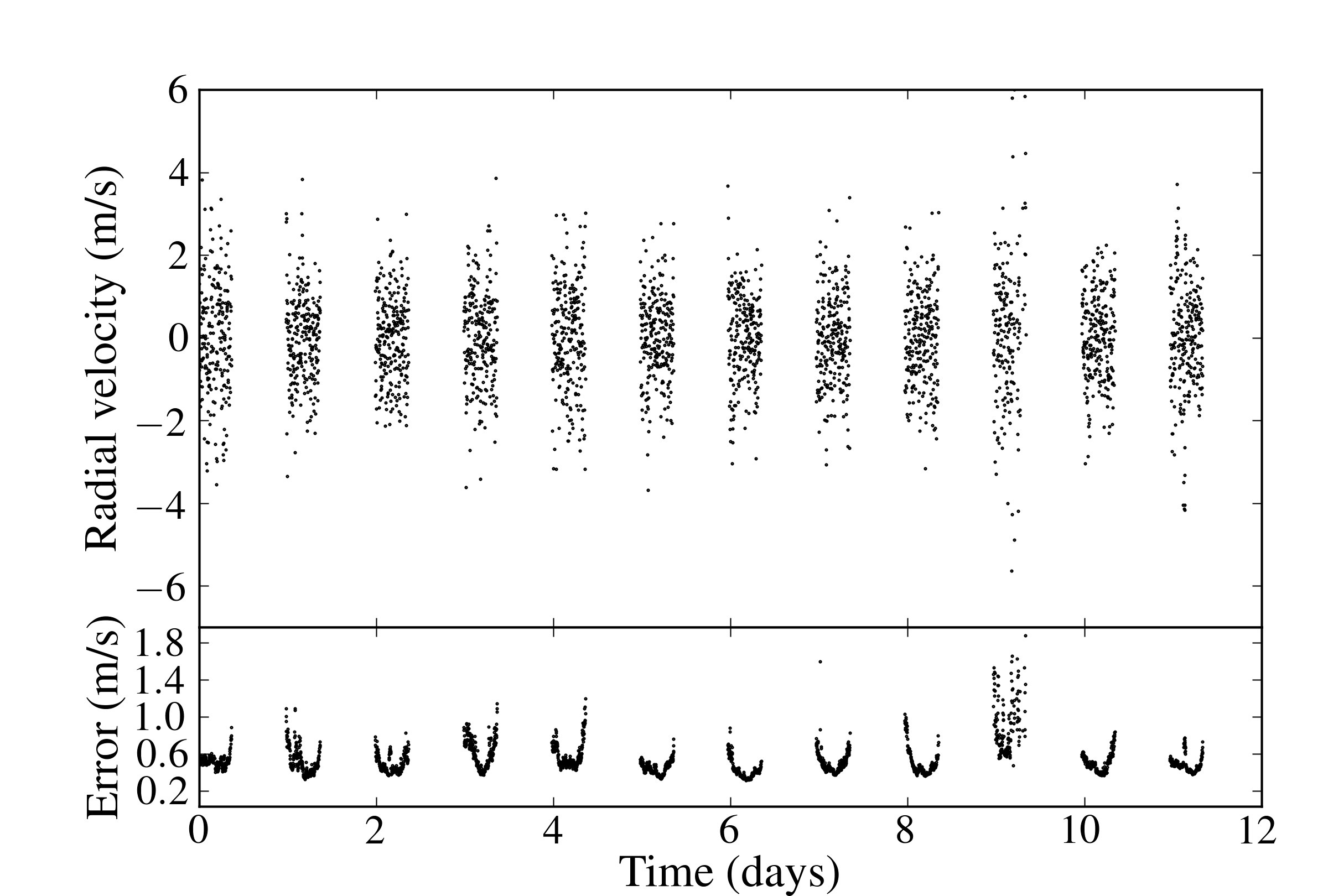
Figure 1: Time series of radial velocities (upper panel) and their uncertainties (lower panel) from HARPS observations of 18 Sco.

The asymptotic relation for high-order p modes is $\nu_{n,l}=(n+l/2+\epsilon_{s})\Delta\nu$, where $\nu_{n,l}$ is the frequency of the mode with radial order $n$ and angular degree $l$, the average large separation $\Delta\nu$ and a surface phase offset $\epsilon_{s}$ (Tassoul 1980). There is a periodicity of $\Delta\nu/2$ in the frequency distribution, implying that there will be a local maximum at this value in the autocorrelation function (ACF) of the signal $y(t)$, defined by $R_{yy}(\tau)=E[y^{\ast}(t)y(t+\tau)]$ (where $E$ is the expectation value and $y^{\ast}$ the complex conjugate of $y$). The ACF for 18 Sco is shown in Fig. 3. Since the signal is irregularly sampled with daily gaps, it was computed by applying the Wiener-Khinchine theorem.

The large separation estimator is thus simply

$$\tilde{\Delta\nu}=\displaystyle 2\times[\underset{t\in\mathscr{T}}{\operatorname{argmax}}(R_{yy}\ast H)]^{-1},$$ (1)

where $\mathscr{T}$ is the domain in which we search for this maximum, which we set at $\mathscr{T}=[13000,25000]$ s (i.e. in the frequency range 40-80 $\mu$Hz), and $H$ the Fourier transform of a filter $h(\nu)$ that truncates the power spectrum. Indeed, only the range 1500-3700 $\mu$Hz is considered when computing (using an FFT algorithm) the Fourier transform of the spectrum. We used zero-padding to ensure that the ACF was evaluated at points separated by an “equivalent frequency resolution” $\sim$0.01 $\mu$Hz. As noted by Roxburgh (2009), the width of $h(\nu)$ affects the localization of $\tilde{\Delta\nu}$, which is a limitation of the method.

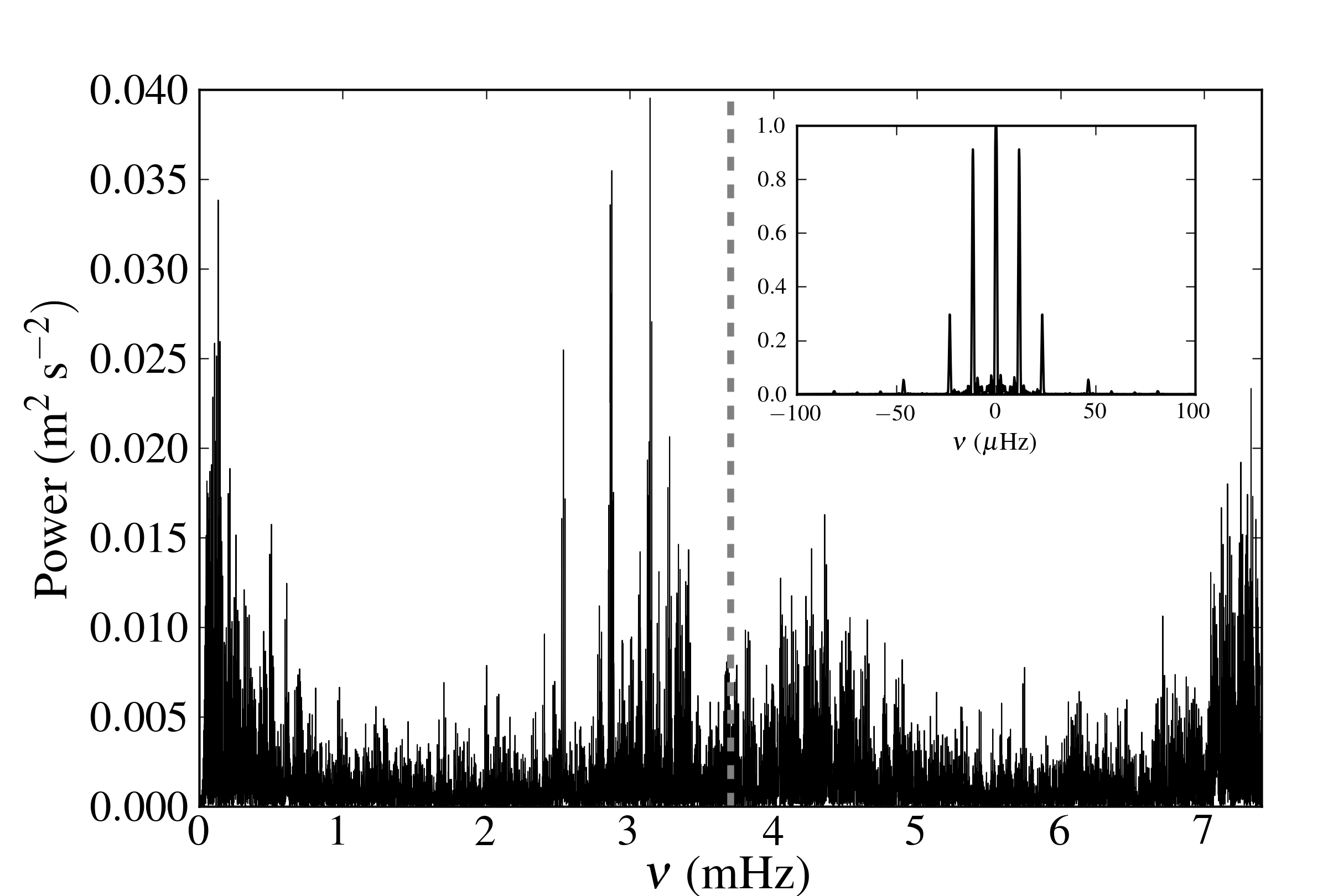
Figure 2: Power spectrum of 18 Sco, evaluated using a weighted Lomb-Scargle “periodogram”. The vertical grey dashed line marks the location of the equivalent Nyquist frequency. The inset shows the spectral window $W$, normalized to its maximum.

The next step is to obtain information about the statistical properties of the estimator $\tilde{\Delta\nu}$ that accounts for the noise in the data. We can write

$$\boldsymbol{y}=\boldsymbol{x}+\boldsymbol{\varepsilon},$$ (2)

where $\boldsymbol{y}=[y_{0},\dots,y_{N}]$ are the measured values of the radial velocity at times $t_{0},\dots,t_{N}$, $\boldsymbol{x}=[x_{0}\dots,x_{N}]$ are the true values of the radial velocity and $\boldsymbol{\varepsilon}=[\varepsilon_{0},\dots,\varepsilon_{N}]$ is a vector gathering the noise contributions from observational errors. Our goal is to estimate the probability density of $\tilde{\Delta\nu}$ conditional on $\boldsymbol{y}$, $p(\tilde{\Delta\nu}|\boldsymbol{y})$. To do so, we used a Monte Carlo approach to error propagation. We assumed that the noise in the data is a series of realizations of independent random variables distributed according to the Gaussian distributions $\mathcal{N}_{i}=\mathcal{N}(x(t_{i}),\sigma_{i}^{2})$, with the $\sigma_{i}$ given by the uncertainties on the data. We simulated time series by generating new realizations of the noise distributed according to the $\mathcal{N}_{i}$ at each $t_{i}$ and adding them to $y_{i}$. For each artificial set of data $\boldsymbol{y^{a}}$, we estimated $\tilde{\Delta\nu^{a}}$.

Our process for generating the artificial data means that it satisfies

$$\boldsymbol{y^{a}}=\boldsymbol{y}+\boldsymbol{\varepsilon^{\prime}}=\boldsymbol{x}+\boldsymbol{\varepsilon}+\boldsymbol{\varepsilon^{\prime}},$$ (3)

with $\boldsymbol{\varepsilon^{\prime}}$ the artificially generated noise, and $\boldsymbol{\varepsilon^{\prime}}$ and $\boldsymbol{\varepsilon}$ both realizations of the same distribution at time $t_{i}$. Ideally, one wishes to estimate the large separation from $\boldsymbol{x}$. One possibility would be to estimate it from several measurements, on different telescopes at the same times $t_{i}$. A second way would be to generate the $\boldsymbol{y^{a}}$ from a model reproducing the data $\boldsymbol{y}$, then perturbing the output of this model, rather than the real observations, which is the classical procedure of Monte Carlo estimation of parameters. Unfortunately, the knowledge of $\Delta\nu$ alone does not permit such a model to be set up.

It thus has to be assumed that this bias will not be too severe, which can be crudely checked graphically with an échelle diagram (see Fig. 4). Further estimations of the large separations, using individual frequencies, may give us some information on its magnitude. However, the error bars are representative of the error propagation: were we able to correct for the bias induced by random observational noise, we would expect our confidence interval on the large separation to be the same.

Figure 4 shows the results for our Monte Carlo suite of 10000 time series. It closely follows a Gaussian distribution with parameters $\mu=134.4$ $\mu$Hz and $\sigma=0.3$ $\mu$Hz. The right panel represents the échelle diagram of the observations using this value for the mean large separation.

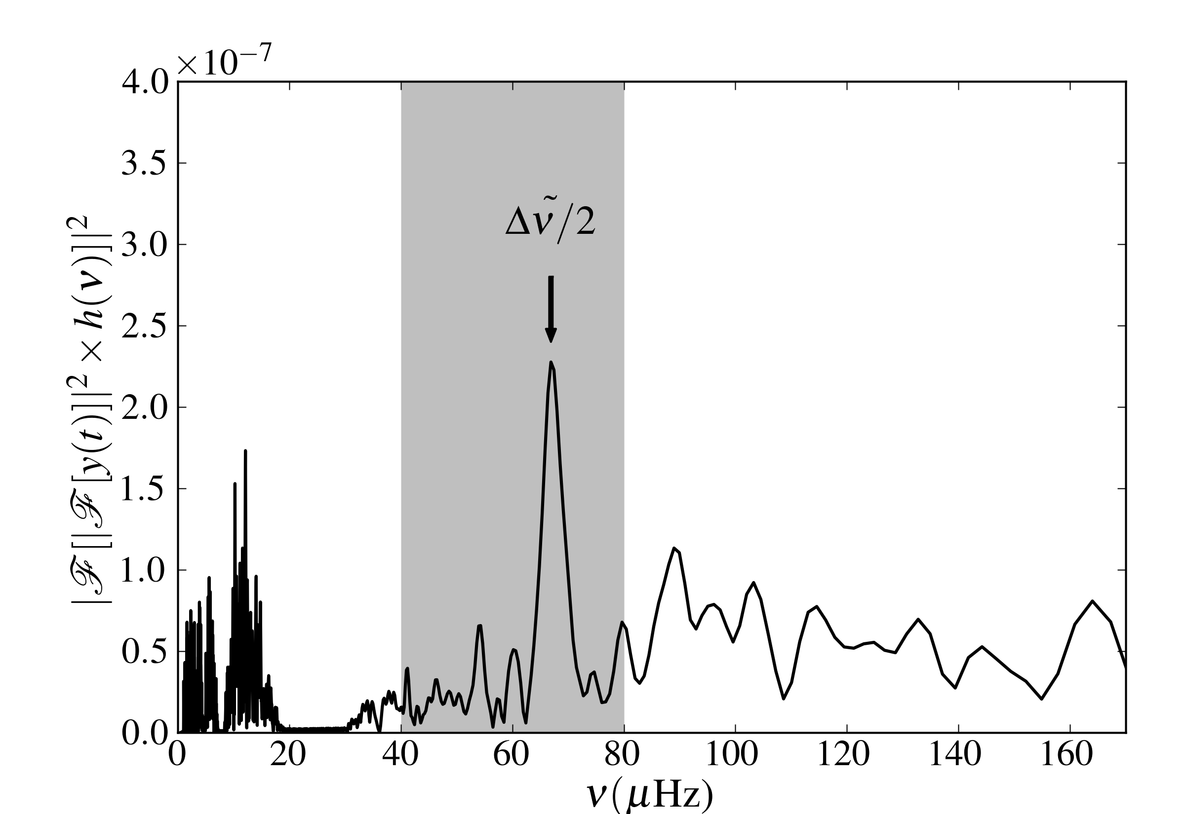
Figure 3: Filtered autocorrelation function for the observed data. The shaded area marks the interval $\mathscr{T}$, in which we searched for the local maximum corresponding to $\Delta\nu/2$. $\mathscr{F}$ is the Fourier transform.

3 Interferometry

To measure the angular diameter of 18 Sco, which is expected to only be about 0.7 mas, we used long-baseline interferometry at visible wavelengths. We used the PAVO beam combiner (Precision Astronomical Visible Observations; Ireland et al. 2008) at the CHARA array (Center for High Angular Resolution Astronomy; ten Brummelaar et al. 2005). We obtained four calibrated sets of observations on 18 July 2009 using the S1-W2 (211 m) baseline.

PAVO records fringes in 38 wavelength channels centred on the $R$ band ($\lambda_{c}\simeq 700$ nm). The raw data were reduced using the PAVO data analysis pipeline (M. J. Ireland et al. in preparation). To enhance the signal-to-noise ratio, the analysis pipeline can average over several wavelength channels, and for 18 Sco we found an optimal smoothing width of five channels. Excluding four channels on each end because of edge effects, this resulted in six independent data points per scan and hence a total of 24 independent visibility measurements for 18 Sco.

Table 1 lists the three stars we used to calibrate the visibilities. We estimated their angular diameters, $\theta$, using the $V$–$K$ calibration of Kervella et al. (2004). Although the internal precision of this calibration, as well as the uncertainties in the photometry for all three stars, is better than 1%, we assume here conservative uncertainties of 5% for each calibrator (van Belle & van Belle 2005). These incorporate the unknown orientation and expected oblateness in fast rotators (Royer et al. 2002). These were chosen to be single stars with predicted diameters at least a factor of two smaller than 18 Sco and to be nearby on the sky (at a separation $d<10\degr$). Each of the four scans of 18 Sco was calibrated, using a weighted mean of the calibrators bracketing the scan. All scans contributing to a bracket were made within a time interval of 15 minutes. The final calibrated squared-visibility measurements are shown in Fig. 5 as a function of spatial frequency.

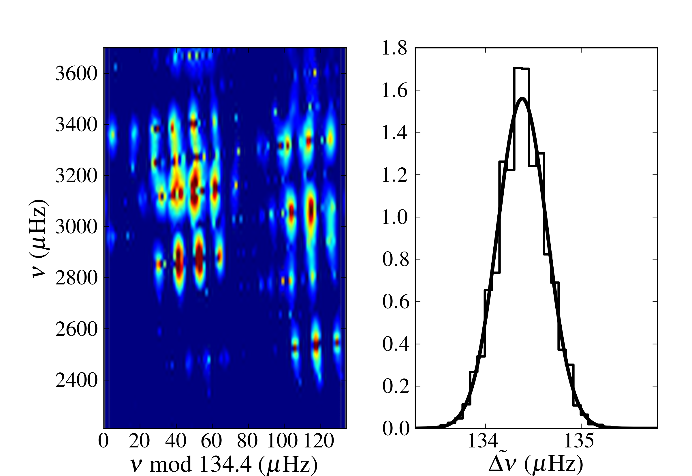
Figure 4: Left panel: échelle diagram corresponding to the mean value of $\tilde{\Delta\nu}$. Right panel: results from the Monte Carlo experiment. The histogram shows the distribution of the actual realizations, and the continuous line the Gaussian with the corresponding mean and variance.

To determine the angular diameter, corrected for limb darkening, we fitted the following model to the data (Hanbury Brown et al. 1974):

$$V=\left(\frac{1-\mu_{\lambda}}{2}+\frac{\mu_{\lambda}}{3}\right)^{-1}\left[(1-\mu_{\lambda})\frac{J_{1}(x)}{x}+\mu_{\lambda}(\pi/2)^{1/2}\frac{J_{3/2}(x)}{x^{3/2}}\right]$$ (4)

with $x=\pi B\theta_{\mathrm{LD}}\lambda^{-1}$. Here, $V$ is the visibility, $\mu_{\lambda}$ the linear limb-darkening coefficient, $J_{n}(x)$ the $n$-th order Bessel function, $B$ the projected baseline, $\theta_{\mathrm{LD}}$ the limb-darkened angular diameter, and $\lambda$ the wavelength at which the observations were done. In our analysis, we used $\mu_{\lambda}=0.607\pm 0.012$, which is interpolated at the $T_{\mathrm{eff}}$, $\log g$, and metallicity of 18 Sco in the R-filter given in the catalog of Claret (2000). For all wavelength channels, we assumed an absolute error of 5nm ($\sim$0.5%).

Interferometric measurements are often dominated by systematic errors and therefore require a careful analysis of all error sources. To arrive at realistic uncertainties for the angular diameter, we performed a series of $10^{4}$ Monte Carlo simulations as follow. For each simulation, we drew realizations from the observed values (assuming they correspond to the parameters of Gaussian distributions) for the calibrator angular diameters, limb darkening coefficient, and wavelength channels. With these parameters we then calibrated the raw visibility measurements and fit the angular diameter $\theta_{\mathrm{LD}}$ to the calibrated data using a least-squares minimization algorithm. Finally, we generated for each simulation a random sample of 200 normally distributed points with a mean corresponding to the fitted diameter and a standard deviation corresponding to the formal uncertainty (scaled so that $\chi^{2}=1$) of the fit. For each Monte-Carlo simulation these 200 points were stored to make up the final distribution containing $2\times 10^{6}$ points. This procedure was carried out for all independent measurements in our data.

The resulting distribution for the diameter of 18 Sco is shown in Fig. 5, along with the best-fitting model. The mean and standard deviation of this distribution yield $\theta_{\mathrm{LD}}=0.6759\pm 0.0062$ mas. Combined with the Hipparcos parallax of $71.94\pm 0.37$ mas (van Leeuwen 2007), we find the radius of 18 Sco to be $R/R_{\odot}=1.010\pm 0.009$. We conclude that the radius of 18 Sco is the same as the Sun, within an uncertainty of 0.9%.

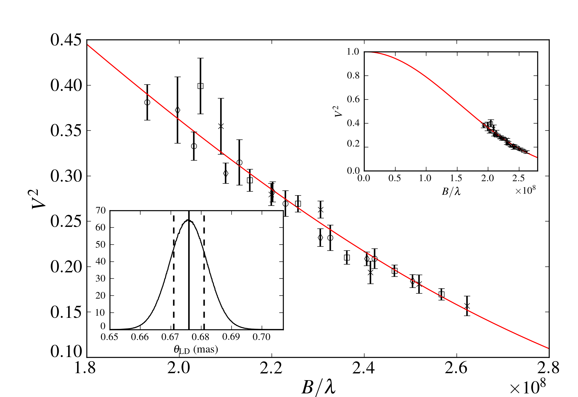
Figure 5: Calibrated squared visibilities for 18 Sco. The red line represents the best model. Each symbol type corresponds to one scan, the visibility averaged over five wavelength channels. Upper-right inset: Same model represented on a larger scale. Lower-left inset: distribution for angular diameter (mean and standard deviation represented by vertical lines).

Table 1: Properties of the calibrators used for 18 Sco.

Star	$V$	$K$	Sp. Type	$\theta$ (mas)	$d$ (deg)
HD145607	5.435	5.052	A4V	0.343$\pm$0.017	0.9
HD145788	6.255	5.737	A1V	0.256$\pm$0.013	4.2
HD147550	6.245	5.957	B9V	0.233$\pm$0.012	6.5

4 Mass of 18 Sco

Gough (1990) pointed out that the homology relation:

$$\Delta\nu\propto M^{1/2}R^{-3/2},$$ (5)

holds for main-sequence stars even outside the zero-age main sequence. Other studies have confirmed this picture (e.g., Stello et al. 2009).

Applying the ACF method described above to a one-year BiSON time series of the Sun (Broomhall et al. 2009, and references therein), we found the solar large separation to be $135.229\pm 0.003$ $\mu$Hz. With our radius measurement this gives a mass $M=1.02\pm 0.03$ M_⊙ for 18 Sco. The agreement is good with the published estimates derived from indirect methods, such as comparison between spectro- or photometric observations and stellar evolutionary tracks (Valenti & Fischer 2005; Meléndez & Ramírez 2007; Takeda et al. 2007; Sousa et al. 2008; do Nascimento et al. 2009).

The assumption of homology is in general well-supported by the comparison to models. Considering a small departure from it in the form $\Delta\nu\propto(1+c)M^{1/2}R^{-3/2}$ (with $c\ll 1$, being a function of the structure of the star), we then have for a scaling relative to the Sun, $c=(\Delta\nu/\Delta\nu_{\odot})(M/M_{\odot})^{1/2}(R/R_{\odot})^{-3/2}-1$. For stellar ages characteristics of those quoted for 18 Sco (the dependence on the mass and the metallicity being weak), this quantity may contribute to an additional $\sim$0.2%-0.4% on the total error on the mass.

The impact of filtering the ACF is not completely negligible, and if we vary the lower limit of $\mathscr{T}$, between 1500 $\mu$Hz and 2000 $\mu$Hz, the final estimate may vary by $\sim$0.01 M_⊙, emphasizing the need for individual frequency measurements.

5 Conclusion

We presented the first asteroseismic and interferometric measurements for the solar twin 18 Sco. These allowed us to estimate a mass for this star independent of the previous spectro-photometric studies, which are still being confirmed. This work shows the possibilities offered by asteroseismology, even from a ground-based single site, and iby nterferometry. Our results confirm that 18 Sco is remarkably similar to the Sun in both radius and mass.

The next step will involve measuring the individual oscillation frequencies and performing full modelling using all the available observations. It will hopefully reduce the uncertainty on the estimated age, improving our knowledge of the physical state of 18 Sco (do Nascimento et al. 2009). This will provide a more precise picture of its interior and give information on the depth of its external convective zone (Monteiro et al. 2000), which is necessary if one wishes to study its magnetic activity cycle (Petit et al. 2008).