The wave equation on the extreme Reissner-Nordström black hole

Abstract

We study the scalar wave equation on the open exterior region of an extreme Reissner-Nordström black hole and prove that, given compactly supported data on a Cauchy surface orthogonal to the timelike Killing vector field, the solution, together with its $(t,s,\theta,\phi)$ derivatives of arbitrary order, $s$ a tortoise radial coordinate, is bounded by a constant that depends only on the initial data. Our technique does not allow to study transverse derivatives at the horizon, which is outside the coordinate patch that we use. However, using previous results that show that second and higher transverse derivatives at the horizon of a generic solution grow unbounded along horizon generators, we show that any such a divergence, if present, would be milder for solutions with compact initial data.

1 Introduction

Extreme black holes lie in the boundary between black holes and naked singularities. Since black holes are believed to be astrophysically relevant, whereas naked singularities are considered unphysical, the issue of stability of extreme black holes is key in understanding the process of gravitational collapse. Black hole stability is a longstanding open problem in General Relativity. The pioneering works of Regge, Wheeler [19], Zerilli [23] [22] and Moncrief [17] determined the modal linear stability of electro-gravitational perturbations in the domain of outer communication of the spherically symmetric electro-vacuum black holes, by ruling out exponential growth in time. Since then, a lot of effort has been made to establish more accurate bounds on linear fields. In particular, analyzing the scalar wave equation on the black hole background provides useful insight into the more complex problem of linear gravitational perturbations. Kay and Wald ([20] [21] [15]) obtained uniform boundedness for solutions of the wave equation on the exterior of the Schwarzschild black hole. In recent years this result has been extended to the non-extreme Kerr black hole (see the review articles [8], [9] and references therein.) The purpose of this work is to place pointwise bounds on scalar waves on the exterior region of an extreme Reissner-Nordström black hole. The interest in Reissner-Nordström black holes lies in the fact that they share the complexity of the global structure of the more relevant Kerr black holes and, due to spherical symmetry, are far more tractable than the rotating holes. The modal stability of the outer region of Reissner-Nordström black holes under linear perturbations of the metric and electromagnetic fields was established in [23] [22] [17], both for the extreme and sub-extreme cases. The modal instability of the Reissner-Nordström naked singularity, and also of the black hole inner static region, was proved only recently in [11].

The wave equation on extreme Reissner-Nordström black holes has recently been studied by Aretakis in a series of relevant articles [2, 3, 1], where it was found that second and higher order transverse derivatives at the horizon grow without bound along the horizon generators (see also [16] were similar results were found for the Teukolsky equation on an extreme Kerr black hole). One of the motivations of our article is understanding the meaning of these instabilities. More specifically, we wonder if they arise in the evolution of fields from data of compact support on a $t=$ constant Cauchy surface (“compact data”, for short), which is a subclass in [1, 3, 2] for which, as we show below, the proof of instability there fails. Although we do not prove that the horizon instability is absent for compact data, we do show that, if present, is milder. On the other side, we get a remarkably simple proof of pointwise boundedness of fields of compact data and their partial derivatives of any order in $(t,s,\theta,\phi)$ coordinates on the open black hole exterior region. These results are stated under Theorem 1 in Section 2, where their relevance to the problem of spherical gravitational collapse is discussed. Theorem 1 is proved in Section 3.

2 Main results

Consider the exterior region $\mathcal{D}$ of the extreme Reissner-Nordström black hole. This region is described in isotropic coordinates $(t,\rho,\theta,\phi)$ by the metric

$$g=-N^{-2}dt^{2}+N^{2}\left(d\rho^{2}+\rho^{2}(d\theta^{2}+\sin^{2}\theta d\phi^{2})\right),\;\;N=1+\frac{m}{\rho},$$ (1)

where the positive constant $m$ represents the total mass of the spacetime, which equals the absolute value of the total electric charge. The electromagnetic field

$${\cal F}=\pm\frac{m}{(m+\rho)^{2}}\;dt\wedge d\rho,$$ (2)

together with this metric, solves the Einstein-Maxwell equations. Note that the isotropic coordinate $\rho$ differs from the standard radial coordinate

$$r=\rho+m,$$ (3)

that gives the area $A=4\pi r^{2}$ of the spheres spanned by acting on a point with the $SO(3)$ isometry subgroup. Instead of $\rho$, it is often more convenient to use the “tortoise´´ radial variable $-\infty<s<\infty$ defined by

$$\frac{ds}{d\rho}=N(\rho)^{2}.$$ (4)

We choose the integration constant such that

$$s=\rho-\frac{m^{2}}{\rho}+2m\log\left(\frac{\rho}{m}\right).$$ (5)

Isotropic coordinates cover only the open exterior region $\mathcal{D}$ of the black hole. Figure 1 exhibits the well known conformal diagram of an extreme Reissner-Nordström black hole (see [14], [6] and references therein), region $\mathcal{D}$ appears shaded. The unshaded region is the black hole interior, proved to be linearly unstable in [11]. $S$ is a generic $t=$ constant surface, it is a Cauchy surface for $\mathcal{D}$ and a complete Riemannian manifold with topology $\mathbb{S}^{2}\times\mathbb{R}$. Its induced metric approaches that of the cylinder as $\rho\to 0^{+}$, limit in which the area of the isometry spheres tend to $A=4\pi m^{2}$. We denote by $i_{+}$ and $i_{-}$ the future and past timelike infinity of $\mathcal{D}$ respectively. The asymptotically flat spacelike infinity is denoted by $i_{0}$, and the asymptotically cylindrical end of $t=$ constant surfaces is denoted $i_{c}$. Note that the surface $S$, being orthogonal to the Killing vector $\partial/\partial t$, is asymptotically null at $i_{c}$.

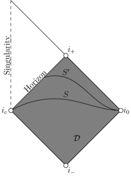
Figure 1: Conformal diagram for the extreme Reissner-Nordström black hole

In this work we study the scalar wave equation on $\mathcal{D}$

$$\Box_{g}\Phi=0,$$ (6)

with initial data on $S$

$$\phi=\Phi|_{S},\quad\chi=\dot{\Phi}|_{S},$$ (7)

where the dot denotes derivative with respect to $t$. The existence and uniqueness of the solution of the Cauchy problem (6)-(7) on a curved background is well established (see, for example, [14], also [12]). We prove the following

Theorem 1.

Let $\Phi$ be a solution of the wave equation (6) on the open exterior region $\mathcal{D}$ of an extreme Reissner-Nordström black hole, which has smooth initial data (7) of compact support on the Cauchy surface $S$. Then, there exists a constant $C$, which depends only on the initial data (7), such that, in $\mathcal{D}$,

$$|\Phi|\leq\frac{C}{\rho+m}.$$ (8)

All higher partial derivatives with respect to the coordinates $(t,s,\theta,\phi)$ are similarly bounded in $\mathcal{D}$. Namely, for any $\alpha_{1}\alpha_{2}...$ there exists a constant $C_{\alpha_{1}\alpha_{2}....}$ that depends on the initial data, such that

$$|\partial_{\alpha_{1}}\partial_{\alpha_{2}}...\Phi|\leq\frac{C_{\alpha_{1}\alpha_{2}...}}{\rho+m}.$$ (9)

Theorem 1 establishes that the spacetime $\mathcal{D}$ is stable with respect to this class of initial data. A key simplification in the study of extreme black holes, compared to non-extreme ones, is the existence of complete exterior Cauchy surfaces such as $S$. This has been extensively used in the present work because it allows us to avoid the delicate issues related to the behaviour of fields near the horizon. We should stress that theorem 1 applies to the evolution of data with compact support on $S$. By finite speed propagation, it is clear that the restriction of $\Phi$ to any $t=$ constant slice will have compact support, and, by smoothness, it will be bounded. The non-trivial statement in Theorem 1 is that there exists a $t$-independent bound for $\Phi$.

The scalar wave equation on the exterior of an extreme Reissner-Nordström black hole has recently been treated by Aretakis in [1], [3] and [2] by evolving data from a non-Cauchy surface such as $S^{\prime}$ in Figure 1. This surface intersects the horizon on one end, goes to spacelike infinity on the other end, and is suitable to analyze the stability of the exterior region of a spherical collapse of an extreme charged body (see Figure 2). Among the many estimates found in these articles, two of them relate closely to our result. The first one is the pointwise boundedness of the solution in the domain of dependence of $S^{\prime}$, in terms of initial data on $S^{\prime}$, given in Theorem 4 in [3]. A weaker bound than (8), $|\Phi|<C$, follows from this theorem and the fact that, for the kind of initial data we consider, $\Phi$ has compact support $K$ in the region between $S$ and $S^{\prime}$. There are, however, two important motivations to study compact data fields. The first one is that the proof of Theorem 1 is considerably simpler than the boundedness proof in [2], since it uses uses only arguments involving the canonical conserved energy of the wave equation, this being possible due to the existence of the above mentioned complete Cauchy surface. The cost of this simplification is that the results in [3] apply to a wider class of data on $S^{\prime}$ than those coming from the evolution of fields with compact support on $S$, as we discuss below.

The second motivation is determining if the blow up result for second and higher transverse derivatives at the horizon along the horizon generators, reported in Theorem 6 in [3], and generalized to scalar wave equations on spacetimes with degenerate Killing horizons in [4], holds for compact data. To state this result we need to switch to a coordinate system that covers the horizon:

$$\{v=t+s(\rho),r=\rho+m,\theta,\phi\}.$$ (10)

In these coordinates the metric (1) has the form

$$g=-(1-m/r)^{2}\;dv^{2}+2dvdr+r^{2}\;(d\theta^{2}+\sin^{2}\theta\;d\varphi^{2}),$$ (11)

and the entire diagram in Figure 1 is covered. The horizon is located at $r=m$, and region ${\cal D}$ corresponds to $r>m$. The Killing vector field $\partial/\partial v$ becomes null at $r=m$, its integral lines are the horizon generators, and $v$ is an affine parameter. Note that $\partial/\partial r|_{r=m}$ is a null vector, orthogonal to the $SO(3)$ orbits, and has unit inner product with $\partial/\partial v$. We call $\partial/\partial r|_{r=m}$ a transverse derivative at the horizon. Theorem 6 in [3] states that second and higher order transverse derivatives of a solution of the scalar field equation diverge as $v\to\infty$ along horizon generators. Although this result holds for generic data in the class analyzed therein, it fails for those fields which evolve from data with compact support on $S$, as we discuss in detail in Section 3.6.1. For fields evolving from compact data, we could not rule out these divergences, although we showed that, if present, they would be milder than those reported by Aretakis.

In what follows we analyze the behaviour of fields with initial data with compact support on $S$ of Figure 1. Consider the spherically symmetric collapse of charged matter. It is possible to arrange the matter model in such a way that the exterior region is a portion of an extreme Reissner-Nordström black hole. One way of constructing such spacetime is by using a thin shell of matter, this has been extensively studied in [5]. Other models are those of charged dust collapse (see [18] and references therein). For the present discussion it is enough to know that such a construction is feasible with some matter model. We show schematically the conformal diagram of a charged collapse spacetime in Figure 2, where we have avoided drawing the singularity, which may have a complicated structure, irrelevant to our purposes.

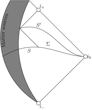
Figure 2: Conformal diagram for the collapse of charged dust.

In a realistic collapse of matter there is always a surface like $S^{\prime}$, for which the intersection ${\cal I}$ of its future domain of dependence with the domain of outer communications agrees with that of $S^{\prime}$ in Figure 1. Note that the results in [2, 3] apply to ${\cal I}$ for data given on $S^{\prime}$ which may be non trivial at the horizon. In Figure 2, $S$ is a Cauchy surface of $\mathbb{R}^{3}$ topology that enters the matter region, and $\Sigma\subset S$ is the minimal subset of $S$ whose future contains $S^{\prime}$. The results [2, 3] imply that generic data of compact support within the vacuum region of $S$ will evolve in a bounded wave in the vacuum portion of this spacetime outside the horizon. This is so because the portion of this region lying between $S$ and $S^{\prime}$ is compact and, as the data of this field on $S^{\prime}$ is in the Aretakis class, the field is also bounded in the outer region in the future of $S^{\prime}$.
Our proof of boundedness is simpler, but can only be applied to the spherical collapse model if we restrict to those fields with data of compact support in $\Sigma\subset S$ (instead of $S$), for which the evolution in the outer region is identical to that of a field in the Reissner-Nordström geometry. Physically, these fields are characterized by the fact that they reach the horizon after the surface of the collapsing star has crossed it. We prove below that the growth of these fields along horizon generators is milder than the growth of those fields which enter the matter region earlier. The fact that fields initially supported in $\Sigma$ are better behaved than those entering the matter before the horizon is formed is an aspect of the stability of the spherical collapse worth pointing out.

3 Behaviour of massless scalar fields

3.1 Recasting the wave operator

Consider the wave equation (6) on the exterior ${\cal M}$ of the extreme Reissner-Nordström background, whose metric in isotropic coordinates is (1). Defining

$$\Phi=\frac{F}{(\rho+m)},$$ (12)

we obtain

$$-\tfrac{\rho^{2}}{\rho+m}\;\Box_{g}\Phi=\ddot{F}+\;\mathcal{A}\;F,$$ (13)

where a dot means $\partial_{t}$,

$$\mathcal{A}=-\partial_{s}^{2}+\left(\frac{2m\rho^{3}}{(\rho+m)^{6}}-\frac{\rho^{2}}{(\rho+m)^{4}}\Delta\right)=:-\partial_{s}^{2}+\left(V_{1}-V_{2}\;\Delta\right)$$ (14)

$s$ is the tortoise radial coordinate introduced in (5), and $\Delta$ is the standard Laplacian on the unit sphere. From (5) we deduce

$$s\sim-\frac{m^{2}}{\rho}\;\text{ as }\rho\to 0^{+},\;\;s\sim\rho\;\text{ as }\rho\to\infty.$$ (15)

The potentials $V_{1}$ and $V_{2}$ are positive, bounded

$$0<V_{1}<\frac{1}{32\,m^{2}},\quad 0<V_{2}<\frac{1}{16\,m^{2}},$$ (16)

and have the following fall off

$$V_{2}\sim s^{-2},\quad V_{1}\sim 2m|s|^{-3}\text{ as }s\to\pm\infty.$$ (17)

The symmetry in the asymptotic expressions above is not coincidental, $V$ is an even function of $s$. The origin of this symmetry is the conformal isometry $C$ of extreme Reissner-Nordström noticed in [7], given by

$$C(t,\rho,\theta,\phi)=(t,m^{2}/\rho,\theta,\phi),$$ (18)

Under this map the pullback of the metric and electromagnetic fields are

$$\tilde{g}_{ab}=\left(\tfrac{m}{\rho}\right)^{2}g_{ab},\quad\tilde{\cal F}_{ab}=-{\cal F}_{ab}.$$ (19)

Since the equation $\Box\Phi-(R/6)\Phi$ is conformally invariant with conformal weight minus one, and the Ricci scalar of an electro-vacuum solution vanishes (thus $R=\tilde{R}=0$), it follows that, if $\Phi(t,\rho,\theta,\phi)$ is a solution of $\Box\Phi=0$, then so is

$$^{\prime}\Phi(t,\rho,\theta,\phi)=(m/\rho)\Phi(t,m^{2}/\rho,\theta,\phi).$$ (20)

For the above field ${}^{\prime}F(t,\rho,\theta,\phi)=(\rho+m)(m/\rho)\Phi(t,m^{2}/\rho,\theta,\phi)=F(t,m^{2}/\rho,\theta,\phi)$. The conformal isometry is easily expressed in the alternative radial coordinate $s$: under $\rho\to m^{2}/\rho$, $s\to-s$. The fact that for any solution $F(t,s,\theta,\phi)$ of $(-\partial_{s}^{2}+\left(V_{1}-V_{2}\;\Delta\right)F=0$, the function ${}^{\prime}F(t,s,\theta,\phi)=F(t,-s,\theta,\phi)$ is also a solution of this equation, implies that $V_{i}(s)=V_{i}(-s),i=1,2$.

Note the consistency of the bound (8) with the conformal symmetry: if $\Phi$ has compact support on a $t-$slice, then so does ${}^{\prime}\Phi$ given in (20), however the bound on ${}^{\prime}\Phi$ gives no additional information, as it follows from the bound on $\Phi$:

$$|^{\prime}\Phi(t,\rho,\theta,\phi)|=\left|\frac{m}{\rho}\Phi(t,m2/\rho,\theta,\phi)\right|\leq\frac{m}{\rho}\;\frac{C}{m+(m^{2}/\rho)}=\frac{C}{m+\rho}.$$ (21)

Finally, although we will not make use of this fact, we note that the operator

$$\partial_{s}^{2}+V(s)\Delta,$$ (22)

is the Laplacian on the cylinder ${\cal C}=\mathbb{S}^{2}\times{\mathbb{R}}$ with respect to the metric

$$h=V^{2}ds^{2}+V\;(d\theta^{2}+\sin^{2}\theta d\varphi^{2}),$$ (23)

which reduces to the standard metric on ${\cal C}$ if we set $V(s)=1$. The principal part of the operator $\mathcal{A}$ in (14) is a particular case of (22).

3.2 Estimates for functions defined on the cylinder

A $t-$slice $S$ of the extreme Reissner-Nordström spacetime is a cylinder with the non standard metric induced from (1). In this Section we establish pointwise bounds on functions on $S$ from $L^{2}$ norms defined using the standard metric on $\mathbb{S}^{2}\times{\mathbb{R}}$, i.e., we use the hermitian product

$$\langle f,g\rangle=\int f^{*}\;g\;dx\;\sin(\theta)\,d\theta\,d\varphi,$$ (24)

($x=s/m$, where $s$ is defined in equation (5)) and the associated norm

$$||f||=\mathchoice{{\hbox{$\displaystyle\sqrt{\langle f,f\rangle\,}$}\lower 0.4pt\hbox{\vrule height=7.5pt,depth=-6.00003pt}}}{{\hbox{$\textstyle\sqrt{\langle f,f\rangle\,}$}\lower 0.4pt\hbox{\vrule height=7.5pt,depth=-6.00003pt}}}{{\hbox{$\scriptstyle\sqrt{\langle f,f\rangle\,}$}\lower 0.4pt\hbox{\vrule height=7.5pt,depth=-6.00003pt}}}{{\hbox{$\scriptscriptstyle\sqrt{\langle f,f\rangle\,}$}\lower 0.4pt\hbox{\vrule height=7.5pt,depth=-6.00003pt}}}.$$ (25)

The following result from [10] is used in [15]. Since we will make use of it, we give a detailed proof using elementary methods.

Lemma 1.

Let $f$ be a complex function on the cylinder with finite norm, then

$$|f(s,\theta,\phi)|\leq M\;\left(||f||+m^{2}\,||\partial_{s}^{2}\,f||+||\triangle\,f||\right),$$ (26)

where $M$ is the constant defined in (37).

Proof.

A function $f$ of finite norm can be expanded, using spherical harmonics in $\mathbb{S}^{2}$ and Fourier transform in ${\mathbb{R}}$, as

$$f(x,\theta,\phi)=\frac{1}{\mathchoice{{\hbox{$\displaystyle\sqrt{2\pi\,}$}\lower 0.4pt\hbox{\vrule height=6.44444pt,depth=-5.15558pt}}}{{\hbox{$\textstyle\sqrt{2\pi\,}$}\lower 0.4pt\hbox{\vrule height=6.44444pt,depth=-5.15558pt}}}{{\hbox{$\scriptstyle\sqrt{2\pi\,}$}\lower 0.4pt\hbox{\vrule height=4.51111pt,depth=-3.6089pt}}}{{\hbox{$\scriptscriptstyle\sqrt{2\pi\,}$}\lower 0.4pt\hbox{\vrule height=3.22221pt,depth=-2.57779pt}}}}\int dk\sum_{\ell\,m}\hat{f}_{\ell\,m}(k)\;e^{ikx}\;Y_{\ell\,m}(\theta,\phi).$$ (27)

where

$$\hat{f}_{\ell\,m}(k):=\frac{1}{\mathchoice{{\hbox{$\displaystyle\sqrt{2\pi\,}$}\lower 0.4pt\hbox{\vrule height=6.44444pt,depth=-5.15558pt}}}{{\hbox{$\textstyle\sqrt{2\pi\,}$}\lower 0.4pt\hbox{\vrule height=6.44444pt,depth=-5.15558pt}}}{{\hbox{$\scriptstyle\sqrt{2\pi\,}$}\lower 0.4pt\hbox{\vrule height=4.51111pt,depth=-3.6089pt}}}{{\hbox{$\scriptscriptstyle\sqrt{2\pi\,}$}\lower 0.4pt\hbox{\vrule height=3.22221pt,depth=-2.57779pt}}}}\int dkf(x,\theta,\phi)\;e^{-ikx}\;Y^{*}_{\ell\,m}(\theta,\phi).$$ (28)

From equation (28) we deduce

$$|f(x,\theta,\phi)| \leq\frac{1}{\mathchoice{{\hbox{$\displaystyle\sqrt{2\pi\,}$}\lower 0.4pt\hbox{\vrule height=6.44444pt,depth=-5.15558pt}}}{{\hbox{$\textstyle\sqrt{2\pi\,}$}\lower 0.4pt\hbox{\vrule height=6.44444pt,depth=-5.15558pt}}}{{\hbox{$\scriptstyle\sqrt{2\pi\,}$}\lower 0.4pt\hbox{\vrule height=4.51111pt,depth=-3.6089pt}}}{{\hbox{$\scriptscriptstyle\sqrt{2\pi\,}$}\lower 0.4pt\hbox{\vrule height=3.22221pt,depth=-2.57779pt}}}}\int dk\sum_{\ell\,m}|\hat{f}_{\ell\,m}(k)|\;|Y_{\ell\,m}(\theta,\phi)|$$

$$=\frac{1}{\mathchoice{{\hbox{$\displaystyle\sqrt{2\pi\,}$}\lower 0.4pt\hbox{\vrule height=6.44444pt,depth=-5.15558pt}}}{{\hbox{$\textstyle\sqrt{2\pi\,}$}\lower 0.4pt\hbox{\vrule height=6.44444pt,depth=-5.15558pt}}}{{\hbox{$\scriptstyle\sqrt{2\pi\,}$}\lower 0.4pt\hbox{\vrule height=4.51111pt,depth=-3.6089pt}}}{{\hbox{$\scriptscriptstyle\sqrt{2\pi\,}$}\lower 0.4pt\hbox{\vrule height=3.22221pt,depth=-2.57779pt}}}}\int dk\sum_{\ell\,m}\left[|\hat{f}_{\ell\,m}(k)|(1+k^{2}+\ell(\ell+1))\right]\;\left[\frac{|Y_{\ell\,m}(\theta,\phi)|}{(1+k^{2}+\ell(\ell+1))}\right]$$ (29)

where in the last line we have just multiplied and divided $(1+k^{2}+\ell(\ell+1))$. Using the Cauchy-Schwarz inequality for series in (29), then the Cauchy-Schwarz inequality for integrals yields

$$|f(x,\theta,\phi)| \leq\frac{1}{\mathchoice{{\hbox{$\displaystyle\sqrt{2\pi\,}$}\lower 0.4pt\hbox{\vrule height=6.44444pt,depth=-5.15558pt}}}{{\hbox{$\textstyle\sqrt{2\pi\,}$}\lower 0.4pt\hbox{\vrule height=6.44444pt,depth=-5.15558pt}}}{{\hbox{$\scriptstyle\sqrt{2\pi\,}$}\lower 0.4pt\hbox{\vrule height=4.51111pt,depth=-3.6089pt}}}{{\hbox{$\scriptscriptstyle\sqrt{2\pi\,}$}\lower 0.4pt\hbox{\vrule height=3.22221pt,depth=-2.57779pt}}}}\int dk\mathchoice{{\hbox{$\displaystyle\sqrt{\sum_{\ell\,m}|\hat{f}_{\ell\,m}(k)|^{2}(1+k^{2}+\ell(\ell+1))^{2}\,}$}\lower 0.4pt\hbox{\vrule height=9.30444pt,depth=-7.44359pt}}}{{\hbox{$\textstyle\sqrt{\sum_{\ell\,m}|\hat{f}_{\ell\,m}(k)|^{2}(1+k^{2}+\ell(\ell+1))^{2}\,}$}\lower 0.4pt\hbox{\vrule height=9.30444pt,depth=-7.44359pt}}}{{\hbox{$\scriptstyle\sqrt{\sum_{\ell\,m}|\hat{f}_{\ell\,m}(k)|^{2}(1+k^{2}+\ell(\ell+1))^{2}\,}$}\lower 0.4pt\hbox{\vrule height=7.22223pt,depth=-5.77782pt}}}{{\hbox{$\scriptscriptstyle\sqrt{\sum_{\ell\,m}|\hat{f}_{\ell\,m}(k)|^{2}(1+k^{2}+\ell(\ell+1))^{2}\,}$}\lower 0.4pt\hbox{\vrule height=7.22223pt,depth=-5.77782pt}}}\;\mathchoice{{\hbox{$\displaystyle\sqrt{\sum_{\ell\,m}\frac{|Y_{\ell\,m}(\theta,\phi)|^{2}}{(1+k^{2}+\ell(\ell+1))^{2}}\,}$}\lower 0.4pt\hbox{\vrule height=17.70667pt,depth=-14.16539pt}}}{{\hbox{$\textstyle\sqrt{\sum_{\ell\,m}\frac{|Y_{\ell\,m}(\theta,\phi)|^{2}}{(1+k^{2}+\ell(\ell+1))^{2}}\,}$}\lower 0.4pt\hbox{\vrule height=12.43332pt,depth=-9.9467pt}}}{{\hbox{$\scriptstyle\sqrt{\sum_{\ell\,m}\frac{|Y_{\ell\,m}(\theta,\phi)|^{2}}{(1+k^{2}+\ell(\ell+1))^{2}}\,}$}\lower 0.4pt\hbox{\vrule height=9.5722pt,depth=-7.6578pt}}}{{\hbox{$\scriptscriptstyle\sqrt{\sum_{\ell\,m}\frac{|Y_{\ell\,m}(\theta,\phi)|^{2}}{(1+k^{2}+\ell(\ell+1))^{2}}\,}$}\lower 0.4pt\hbox{\vrule height=9.5722pt,depth=-7.6578pt}}}$$

$$\leq\;\mathchoice{{\hbox{$\displaystyle\sqrt{\sum_{\ell\,m}\int\frac{|Y_{\ell\,m}(\theta,\phi)|^{2}}{(1+k^{2}+\ell(\ell+1))^{2}}\,\frac{dk}{2\pi}\,}$}\lower 0.4pt\hbox{\vrule height=17.70667pt,depth=-14.16539pt}}}{{\hbox{$\textstyle\sqrt{\sum_{\ell\,m}\int\frac{|Y_{\ell\,m}(\theta,\phi)|^{2}}{(1+k^{2}+\ell(\ell+1))^{2}}\,\frac{dk}{2\pi}\,}$}\lower 0.4pt\hbox{\vrule height=12.43332pt,depth=-9.9467pt}}}{{\hbox{$\scriptstyle\sqrt{\sum_{\ell\,m}\int\frac{|Y_{\ell\,m}(\theta,\phi)|^{2}}{(1+k^{2}+\ell(\ell+1))^{2}}\,\frac{dk}{2\pi}\,}$}\lower 0.4pt\hbox{\vrule height=9.5722pt,depth=-7.6578pt}}}{{\hbox{$\scriptscriptstyle\sqrt{\sum_{\ell\,m}\int\frac{|Y_{\ell\,m}(\theta,\phi)|^{2}}{(1+k^{2}+\ell(\ell+1))^{2}}\,\frac{dk}{2\pi}\,}$}\lower 0.4pt\hbox{\vrule height=9.5722pt,depth=-7.6578pt}}}\;\mathchoice{{\hbox{$\displaystyle\sqrt{\sum_{\ell^{\prime}\,m^{\prime}}\int|\hat{f}_{\ell^{\prime}\,m^{\prime}}(k^{\prime})|^{2}\,(1+k^{\prime 2}+\ell^{\prime}(\ell^{\prime}+1))^{2}\;dk^{\prime}\,}$}\lower 0.4pt\hbox{\vrule height=9.30444pt,depth=-7.44359pt}}}{{\hbox{$\textstyle\sqrt{\sum_{\ell^{\prime}\,m^{\prime}}\int|\hat{f}_{\ell^{\prime}\,m^{\prime}}(k^{\prime})|^{2}\,(1+k^{\prime 2}+\ell^{\prime}(\ell^{\prime}+1))^{2}\;dk^{\prime}\,}$}\lower 0.4pt\hbox{\vrule height=9.30444pt,depth=-7.44359pt}}}{{\hbox{$\scriptstyle\sqrt{\sum_{\ell^{\prime}\,m^{\prime}}\int|\hat{f}_{\ell^{\prime}\,m^{\prime}}(k^{\prime})|^{2}\,(1+k^{\prime 2}+\ell^{\prime}(\ell^{\prime}+1))^{2}\;dk^{\prime}\,}$}\lower 0.4pt\hbox{\vrule height=7.22223pt,depth=-5.77782pt}}}{{\hbox{$\scriptscriptstyle\sqrt{\sum_{\ell^{\prime}\,m^{\prime}}\int|\hat{f}_{\ell^{\prime}\,m^{\prime}}(k^{\prime})|^{2}\,(1+k^{\prime 2}+\ell^{\prime}(\ell^{\prime}+1))^{2}\;dk^{\prime}\,}$}\lower 0.4pt\hbox{\vrule height=7.22223pt,depth=-5.77782pt}}}.$$ (30)

The second factor in (30) can be bounded using

$$\langle\partial_{x}^{2}f,\partial_{x}^{2}f\rangle =\int\;dk\;\sum_{\ell\,m}\;|k^{2}\;\hat{f}_{\ell\,m}(k)|^{2},$$ (31)

$$\langle\triangle f,\triangle f\rangle =\int\;dk\;\sum_{\ell\,m}\;|\ell(\ell+1)\;\hat{f}_{\ell\,m}(k)|^{2},$$ (32)

together with $(a+b+c)^{2}\leq 3(a^{2}+b^{2}+c^{2})$ and $\mathchoice{{\hbox{$\displaystyle\sqrt{a^{2}+b^{2}+c^{2}\,}$}\lower 0.4pt\hbox{\vrule height=8.74889pt,depth=-6.99915pt}}}{{\hbox{$\textstyle\sqrt{a^{2}+b^{2}+c^{2}\,}$}\lower 0.4pt\hbox{\vrule height=8.74889pt,depth=-6.99915pt}}}{{\hbox{$\scriptstyle\sqrt{a^{2}+b^{2}+c^{2}\,}$}\lower 0.4pt\hbox{\vrule height=6.14998pt,depth=-4.92001pt}}}{{\hbox{$\scriptscriptstyle\sqrt{a^{2}+b^{2}+c^{2}\,}$}\lower 0.4pt\hbox{\vrule height=4.7611pt,depth=-3.8089pt}}}\leq|a|+|b|+|c|$,

$$\mathchoice{{\hbox{$\displaystyle\sqrt{\sum_{\ell^{\prime}\,m^{\prime}}\int|\hat{f}_{\ell^{\prime}\,m^{\prime}}(k^{\prime})|^{2}\,(1+k^{\prime 2}+\ell^{\prime}(\ell^{\prime}+1))^{2}\;dk^{\prime}\,}$}\lower 0.4pt\hbox{\vrule height=9.30444pt,depth=-7.44359pt}}}{{\hbox{$\textstyle\sqrt{\sum_{\ell^{\prime}\,m^{\prime}}\int|\hat{f}_{\ell^{\prime}\,m^{\prime}}(k^{\prime})|^{2}\,(1+k^{\prime 2}+\ell^{\prime}(\ell^{\prime}+1))^{2}\;dk^{\prime}\,}$}\lower 0.4pt\hbox{\vrule height=9.30444pt,depth=-7.44359pt}}}{{\hbox{$\scriptstyle\sqrt{\sum_{\ell^{\prime}\,m^{\prime}}\int|\hat{f}_{\ell^{\prime}\,m^{\prime}}(k^{\prime})|^{2}\,(1+k^{\prime 2}+\ell^{\prime}(\ell^{\prime}+1))^{2}\;dk^{\prime}\,}$}\lower 0.4pt\hbox{\vrule height=7.22223pt,depth=-5.77782pt}}}{{\hbox{$\scriptscriptstyle\sqrt{\sum_{\ell^{\prime}\,m^{\prime}}\int|\hat{f}_{\ell^{\prime}\,m^{\prime}}(k^{\prime})|^{2}\,(1+k^{\prime 2}+\ell^{\prime}(\ell^{\prime}+1))^{2}\;dk^{\prime}\,}$}\lower 0.4pt\hbox{\vrule height=7.22223pt,depth=-5.77782pt}}}\\ \leq\mathchoice{{\hbox{$\displaystyle\sqrt{\sum_{\ell^{\prime}\,m^{\prime}}\int 3|\hat{f}_{\ell^{\prime}\,m^{\prime}}(k^{\prime})|^{2}\,(1+k^{\prime 4}+\ell^{\prime 2}(\ell^{\prime}+1)^{2})\;dk^{\prime}\,}$}\lower 0.4pt\hbox{\vrule height=9.30444pt,depth=-7.44359pt}}}{{\hbox{$\textstyle\sqrt{\sum_{\ell^{\prime}\,m^{\prime}}\int 3|\hat{f}_{\ell^{\prime}\,m^{\prime}}(k^{\prime})|^{2}\,(1+k^{\prime 4}+\ell^{\prime 2}(\ell^{\prime}+1)^{2})\;dk^{\prime}\,}$}\lower 0.4pt\hbox{\vrule height=9.30444pt,depth=-7.44359pt}}}{{\hbox{$\scriptstyle\sqrt{\sum_{\ell^{\prime}\,m^{\prime}}\int 3|\hat{f}_{\ell^{\prime}\,m^{\prime}}(k^{\prime})|^{2}\,(1+k^{\prime 4}+\ell^{\prime 2}(\ell^{\prime}+1)^{2})\;dk^{\prime}\,}$}\lower 0.4pt\hbox{\vrule height=7.22223pt,depth=-5.77782pt}}}{{\hbox{$\scriptscriptstyle\sqrt{\sum_{\ell^{\prime}\,m^{\prime}}\int 3|\hat{f}_{\ell^{\prime}\,m^{\prime}}(k^{\prime})|^{2}\,(1+k^{\prime 4}+\ell^{\prime 2}(\ell^{\prime}+1)^{2})\;dk^{\prime}\,}$}\lower 0.4pt\hbox{\vrule height=7.22223pt,depth=-5.77782pt}}}=\mathchoice{{\hbox{$\displaystyle\sqrt{3\,}$}\lower 0.4pt\hbox{\vrule height=6.44444pt,depth=-5.15558pt}}}{{\hbox{$\textstyle\sqrt{3\,}$}\lower 0.4pt\hbox{\vrule height=6.44444pt,depth=-5.15558pt}}}{{\hbox{$\scriptstyle\sqrt{3\,}$}\lower 0.4pt\hbox{\vrule height=4.51111pt,depth=-3.6089pt}}}{{\hbox{$\scriptscriptstyle\sqrt{3\,}$}\lower 0.4pt\hbox{\vrule height=3.22221pt,depth=-2.57779pt}}}\mathchoice{{\hbox{$\displaystyle\sqrt{||f||^{2}+||\partial_{x}^{2}\,f||^{2}+||\triangle\,f||^{2}\,}$}\lower 0.4pt\hbox{\vrule height=9.30444pt,depth=-7.44359pt}}}{{\hbox{$\textstyle\sqrt{||f||^{2}+||\partial_{x}^{2}\,f||^{2}+||\triangle\,f||^{2}\,}$}\lower 0.4pt\hbox{\vrule height=9.30444pt,depth=-7.44359pt}}}{{\hbox{$\scriptstyle\sqrt{||f||^{2}+||\partial_{x}^{2}\,f||^{2}+||\triangle\,f||^{2}\,}$}\lower 0.4pt\hbox{\vrule height=6.53888pt,depth=-5.23112pt}}}{{\hbox{$\scriptscriptstyle\sqrt{||f||^{2}+||\partial_{x}^{2}\,f||^{2}+||\triangle\,f||^{2}\,}$}\lower 0.4pt\hbox{\vrule height=5.03888pt,depth=-4.03113pt}}}\\ \leq\mathchoice{{\hbox{$\displaystyle\sqrt{3\,}$}\lower 0.4pt\hbox{\vrule height=6.44444pt,depth=-5.15558pt}}}{{\hbox{$\textstyle\sqrt{3\,}$}\lower 0.4pt\hbox{\vrule height=6.44444pt,depth=-5.15558pt}}}{{\hbox{$\scriptstyle\sqrt{3\,}$}\lower 0.4pt\hbox{\vrule height=4.51111pt,depth=-3.6089pt}}}{{\hbox{$\scriptscriptstyle\sqrt{3\,}$}\lower 0.4pt\hbox{\vrule height=3.22221pt,depth=-2.57779pt}}}\left(||f||+||\partial_{x}^{2}\,f||+||\triangle\,f||\right)$$ (33)

The identity $\sum_{m}|Y_{\ell\,m}(\theta,\phi)|^{2}=(2\ell+1)/(4\pi)$ in the first factor of (30) then gives, after restoring units ($s=mx$),

$$|f(s,\theta,\phi)|\leq M\;\left(||f||+m^{2}\,||\partial_{s}^{2}\,f||+||\triangle\,f||\right),$$ (34)

where

$$M^{2} =\frac{3}{8\pi^{2}}\;\int\sum_{\ell}\frac{2\ell+1}{(1+k^{2}+\ell(\ell+1))^{2}}\,dk$$ (35)

$$=-\frac{3}{8\pi^{2}}\;\frac{\partial}{\partial\ell}\sum_{\ell}\int(1+k^{2}+\ell(\ell+1))^{-1}\,dk$$ (36)

$$=\frac{3}{16\;\pi}\;\sum_{\ell}\frac{2\ell+1}{(1+\ell(\ell+1))^{3/2}}$$ (37)

∎

Applying Lemma 1 to $F_{t}(s,\theta,\phi):=F(t,s,\theta,\phi)$ we get a bound for $|F|$ on the t-slice. However, if the terms $||F_{t}||,||\Delta F_{t}||$ and $||\partial_{s}^{2}\,F_{t}||$ on the right hand side of (26) were further bounded by conserved ($t$-independent) slice integrals, then we would get a $t$-independent bound for $|F_{t}|$, i.e., a bound for $|F|$. This is our motivation to study conserved energies in the following Section.

3.3 Conserved energies

In Section 3.1 we have shown that the problem (6)-(7) of propagation of scalar waves on the exterior extreme Reissner-Nordström spacetime ${\cal M}$ can be reformulated as the equation

$${\cal O}F:=\ddot{F}+\;\mathcal{A}\;F=0,$$ (38)

with initial data $(f,g)$ of compact support on the $t=0$ slice $S=\mathbb{S}^{2}\times\mathbb{R}$, given by

$$f=F(t=0)=\phi/(\rho+m),\quad g=\dot{F}(t=0)=\chi/(\rho+m).$$ (39)

A solution of equation (38) has a conserved (i.e., $t-$independent) energy

$$\mathcal{E}[F]=\int_{S_{t}}(\dot{F}^{2}+F\mathcal{A}(F))\;\,dv,$$ (40)

where the integral is performed on a $t-$slice using the standard volume element $dv=\sin(\theta)\;d\theta\;d\varphi\;ds$. This energy is useful because it provides a $t-$independent bound for $||\partial_{s}F||$.

Taking derivatives with respect to $t$ to equation (38) shows that $\dot{F},\ddot{F},...$ all satisfy the same equation, giving extra conserved quantities, in particular

$$\mathcal{E}[\dot{F}]=\int_{S_{t}}(\ddot{F}^{2}+\dot{F}\mathcal{A}(\dot{F}))\;dv,$$ (41)

which, using (38) to substitute for $\ddot{F}$ reduces to

$$\mathcal{E}[\dot{F}]=\int_{S_{t}}[(\mathcal{A}F)^{2}+\dot{F}\mathcal{A}(\dot{F})]\;\,dv.$$ (42)

The above conserved energy is useful because it provides a $t-$independent bound for $||\mathcal{A}F||$, and thus for $||\partial_{s}^{2}F||$. We would like to get similar bounds for $||(\Delta F)||$ and $||F||$, and use them in (26). Following [8], equation (40) suggests that, to obtain a bound for the integral of $F^{2}$, we should consider the energy of a “time integral” $\tilde{F}$ of the solution $F$ in (38), i.e. a solution of the system

$$\dot{\tilde{F}}=F\;\text{ and }\;\ddot{\tilde{F}}+\;\mathcal{A}\;\tilde{F}=0.$$ (43)

Assume there exists such a solution, its conserved energy would be

$$\mathcal{E}[\tilde{F}] =\int_{S_{t}}\left[(\dot{\tilde{F}})^{2}+\tilde{F}\mathcal{A}(\tilde{F})\right]\,dv,$$ (44)

$$=\int_{S_{t}}\left[F^{2}+\tilde{F}\mathcal{A}(\tilde{F})\right]\,dv,$$ (45)

and would bound $||F||$. Using $[\Delta,{\cal O}]=0$ in (43) we could prove that ${\cal O}\Delta\tilde{F}=0$, the conserved energy of this solution being

$$\mathcal{E}[\Delta\tilde{F}] =\int_{S_{t}}\left(\Delta\dot{\tilde{F}})^{2}+\Delta\tilde{F}\mathcal{A}(\Delta\tilde{F})\right]\,dv,$$ (46)

$$=\int_{S_{t}}\left(\Delta F)^{2}+\Delta\tilde{F}\mathcal{A}(\Delta\tilde{F})\right]\,dv,$$ (47)

which bounds $||\Delta F||$.
In order to proceed with this idea, we have to prove that a solution of (43) exists for $F$ satisfying (38)-(39). This is done in the following Section.

3.4 Integrating in time

In this section we will prove the existence of the “time integral” solution $\tilde{F}$ of the system (43) for a solution $F$ of (38)-(39). The existence of $\tilde{F}$ implies the conservation of the energies (45) and (47) for $F$. The proof requires a notion of the inverse $\mathcal{A}^{-1}$. This is introduced by taking advantage of the fact that ${\cal A}$ is positive definite (since $V_{1}$ and $V_{2}$ are positive), and this allows us to define an inner product on functions on the linear space $\hat{\cal H}$ of functions of compact support on $S$,

$$(p,q)=\int_{S}[\partial_{s}p\partial_{s}q+V_{2}(\partial_{\theta}p\partial_{\theta}q+(\sin\theta)^{-1}\partial_{\phi}p\partial_{\phi}q)+V_{1}pq]\,dv,$$ (48)

which is formally obtained by integrating by parts $\int_{S}p\mathcal{A}q\;dv$. We define a Hilbert space $\mathcal{H}$ as the completion of $\hat{\cal H}$ under this norm. This is the space where $\mathcal{A}^{-1}$ is defined, as shown in the following.

Lemma 2.

Let $q$ be smooth and having compact support $S_{q}\subset S$. Then, there exist a unique solution $p\in\mathcal{H}$ of the equation

$$\mathcal{A}(p)=q.$$ (49)

Moreover, $p$ is smooth.

Proof.

The Lax-Milgram theorem (see for example [13]) asserts that if $B(\cdot,\cdot)$ is a bilinear form on $\mathcal{H}$ for which there exists $\alpha,\beta>0$ such that

$$|B(u,v)|\leq\alpha\mathchoice{{\hbox{$\displaystyle\sqrt{(u,u)\,}$}\lower 0.4pt\hbox{\vrule height=7.5pt,depth=-6.00003pt}}}{{\hbox{$\textstyle\sqrt{(u,u)\,}$}\lower 0.4pt\hbox{\vrule height=7.5pt,depth=-6.00003pt}}}{{\hbox{$\scriptstyle\sqrt{(u,u)\,}$}\lower 0.4pt\hbox{\vrule height=5.25pt,depth=-4.20003pt}}}{{\hbox{$\scriptscriptstyle\sqrt{(u,u)\,}$}\lower 0.4pt\hbox{\vrule height=3.75pt,depth=-3.00002pt}}}\;\mathchoice{{\hbox{$\displaystyle\sqrt{(v,v)\,}$}\lower 0.4pt\hbox{\vrule height=7.5pt,depth=-6.00003pt}}}{{\hbox{$\textstyle\sqrt{(v,v)\,}$}\lower 0.4pt\hbox{\vrule height=7.5pt,depth=-6.00003pt}}}{{\hbox{$\scriptstyle\sqrt{(v,v)\,}$}\lower 0.4pt\hbox{\vrule height=5.25pt,depth=-4.20003pt}}}{{\hbox{$\scriptscriptstyle\sqrt{(v,v)\,}$}\lower 0.4pt\hbox{\vrule height=3.75pt,depth=-3.00002pt}}},\;\;(u,u)\leq\beta\;B(u,u),$$ (50)

hold for all $u,v\in\mathcal{H}$ then, for any bounded linear operator $L:\mathcal{H}\to{\mathbb{R}}$, the equation on $p$

$$B(z,p)=L(z)\;\;\text{ for every }\;z\in\mathcal{H},$$ (51)

has a unique solution.
Conditions (50) are trivially satisfied for $\alpha=\beta=1$ if $B(p,q)=(p,q)$ (Schwarz’s inequality).

The operator $L(z):=\int_{S}qz\;dv$ can be shown to be bounded by using the fact that the restriction of $V_{1}$ to $S_{q}$ has a minimum $V_{1}^{(q)}>0$ and thus, applying Schwarz’s inequality to $L^{2}[{\cal S}_{q},dv]$ gives

$$|L(z)|=\left|\int_{{S}_{q}}qz\;dv\right|\leq\mathchoice{{\hbox{$\displaystyle\sqrt{\int_{{S}_{q}}q^{2}\;dv\,}$}\lower 0.4pt\hbox{\vrule height=6.94444pt,depth=-5.55559pt}}}{{\hbox{$\textstyle\sqrt{\int_{{S}_{q}}q^{2}\;dv\,}$}\lower 0.4pt\hbox{\vrule height=6.94444pt,depth=-5.55559pt}}}{{\hbox{$\scriptstyle\sqrt{\int_{{S}_{q}}q^{2}\;dv\,}$}\lower 0.4pt\hbox{\vrule height=4.8611pt,depth=-3.8889pt}}}{{\hbox{$\scriptscriptstyle\sqrt{\int_{{S}_{q}}q^{2}\;dv\,}$}\lower 0.4pt\hbox{\vrule height=3.47221pt,depth=-2.77779pt}}}\;\mathchoice{{\hbox{$\displaystyle\sqrt{\int_{{S}_{q}}z^{2}\;dv\,}$}\lower 0.4pt\hbox{\vrule height=6.94444pt,depth=-5.55559pt}}}{{\hbox{$\textstyle\sqrt{\int_{{S}_{q}}z^{2}\;dv\,}$}\lower 0.4pt\hbox{\vrule height=6.94444pt,depth=-5.55559pt}}}{{\hbox{$\scriptstyle\sqrt{\int_{{S}_{q}}z^{2}\;dv\,}$}\lower 0.4pt\hbox{\vrule height=4.8611pt,depth=-3.8889pt}}}{{\hbox{$\scriptscriptstyle\sqrt{\int_{{S}_{q}}z^{2}\;dv\,}$}\lower 0.4pt\hbox{\vrule height=3.47221pt,depth=-2.77779pt}}}\\ <\mathchoice{{\hbox{$\displaystyle\sqrt{\int_{{S}_{q}}q^{2}\;dv\,}$}\lower 0.4pt\hbox{\vrule height=6.94444pt,depth=-5.55559pt}}}{{\hbox{$\textstyle\sqrt{\int_{{S}_{q}}q^{2}\;dv\,}$}\lower 0.4pt\hbox{\vrule height=6.94444pt,depth=-5.55559pt}}}{{\hbox{$\scriptstyle\sqrt{\int_{{S}_{q}}q^{2}\;dv\,}$}\lower 0.4pt\hbox{\vrule height=4.8611pt,depth=-3.8889pt}}}{{\hbox{$\scriptscriptstyle\sqrt{\int_{{S}_{q}}q^{2}\;dv\,}$}\lower 0.4pt\hbox{\vrule height=3.47221pt,depth=-2.77779pt}}}\;\mathchoice{{\hbox{$\displaystyle\sqrt{\int_{{S}_{q}}\left(\frac{V_{1}}{V_{1}^{(q)}}\right)z^{2}\;dv\,}$}\lower 0.4pt\hbox{\vrule height=14.00664pt,depth=-11.20537pt}}}{{\hbox{$\textstyle\sqrt{\int_{{S}_{q}}\left(\frac{V_{1}}{V_{1}^{(q)}}\right)z^{2}\;dv\,}$}\lower 0.4pt\hbox{\vrule height=9.8583pt,depth=-7.88669pt}}}{{\hbox{$\scriptstyle\sqrt{\int_{{S}_{q}}\left(\frac{V_{1}}{V_{1}^{(q)}}\right)z^{2}\;dv\,}$}\lower 0.4pt\hbox{\vrule height=7.8083pt,depth=-6.24667pt}}}{{\hbox{$\scriptscriptstyle\sqrt{\int_{{S}_{q}}\left(\frac{V_{1}}{V_{1}^{(q)}}\right)z^{2}\;dv\,}$}\lower 0.4pt\hbox{\vrule height=7.8083pt,depth=-6.24667pt}}}<\mathchoice{{\hbox{$\displaystyle\sqrt{\int_{{S}_{q}}\left(\frac{q^{2}}{V_{1}^{(q)}}\right)\;dv\,}$}\lower 0.4pt\hbox{\vrule height=13.42331pt,depth=-10.7387pt}}}{{\hbox{$\textstyle\sqrt{\int_{{S}_{q}}\left(\frac{q^{2}}{V_{1}^{(q)}}\right)\;dv\,}$}\lower 0.4pt\hbox{\vrule height=9.44997pt,depth=-7.56001pt}}}{{\hbox{$\scriptstyle\sqrt{\int_{{S}_{q}}\left(\frac{q^{2}}{V_{1}^{(q)}}\right)\;dv\,}$}\lower 0.4pt\hbox{\vrule height=7.51663pt,depth=-6.01334pt}}}{{\hbox{$\scriptscriptstyle\sqrt{\int_{{S}_{q}}\left(\frac{q^{2}}{V_{1}^{(q)}}\right)\;dv\,}$}\lower 0.4pt\hbox{\vrule height=7.51663pt,depth=-6.01334pt}}}\;\mathchoice{{\hbox{$\displaystyle\sqrt{(z,z)\,}$}\lower 0.4pt\hbox{\vrule height=7.5pt,depth=-6.00003pt}}}{{\hbox{$\textstyle\sqrt{(z,z)\,}$}\lower 0.4pt\hbox{\vrule height=7.5pt,depth=-6.00003pt}}}{{\hbox{$\scriptstyle\sqrt{(z,z)\,}$}\lower 0.4pt\hbox{\vrule height=5.25pt,depth=-4.20003pt}}}{{\hbox{$\scriptscriptstyle\sqrt{(z,z)\,}$}\lower 0.4pt\hbox{\vrule height=3.75pt,depth=-3.00002pt}}}$$ (52)

It follows from the Lax-Milgram theorem that there exists a $p\in\mathcal{H}$ such that

$$\int_{S}z\mathcal{A}p\;dv=\int_{S}zq\;dv,\;\;\text{ for every }\;z\in\mathcal{H},$$ (53)

and hence $p$ is a weak solution of the elliptic differential equation $\mathcal{A}p=q$. Smoothness of $p$ follows from interior elliptic regularity arguments (see [13]) and thus $p$ satisfies $\mathcal{A}p=q$.

∎

An alternative proof using expansions in spherical harmonics $Y_{\ell m}(\theta,\phi)$ sheds light on the behaviour of $p$ at infinity and near the horizon. Introducing $P=p/N$, equation (49) reads

$$\mathcal{A}(p)=\mathcal{A}(NP)=N^{-3}\left(\partial^{2}_{\rho}P+r^{-2}\triangle P\right)=q.$$ (54)

If we expand $P=\sum_{\ell m}P_{\ell m}(\rho)Y_{\ell m}(\theta,\phi)$ (and similarly expand $q$) the above equation reduces to an ODE for each mode that can solved explicitly:

$$(2\ell+1)\,P_{\ell m}(\rho)=\rho^{\ell+1}\int^{\rho}_{C_{\ell m}}x^{-\ell}N^{3}(x)q_{\ell m}(x)\,dx-\rho^{-\ell}\int^{\rho}_{D_{\ell m}}x^{\ell+1}N^{3}(x)q_{\ell m}(x)\,dx.$$ (55)

For every harmonic mode, $C_{\ell m}$ and $D_{\ell m}$ are constants of integration of the generic solution above, however if we use the fact that the $q_{\ell m}$ have compact support, we conclude that the choice $C_{\ell m}=\infty,D_{\ell m}=0$ is the only one that gives an appropriate asymptotic behavior near the horizon and spatial infinity, such that $p$ belongs to $\mathcal{H}$. This gives (after multiplication times $N$) the unique $p$ singled out by the Lax-Milgram theorem. Its projection

$$p_{\ell}:=\sum_{m=-\ell}^{\ell}p_{\ell m}(\rho)Y_{\ell m}(\theta,\phi),$$ (56)

onto the $\ell$ subspace behaves as

$$p_{\ell}\sim\begin{cases}\rho^{\ell}&\text{ as }\rho\to 0^{+},\\ \rho^{-\ell}&\text{ as }\rho\to\infty.\end{cases}$$ (57)

Thus, generically, $p$ approaches a constant in both the $\rho\to\infty$ and the $\rho\to 0^{+}$ limits.

Lemma 2 refer to the space variables on the cylinder $S$, however the functions involved in the proof of existence of equations (43) depend also on the time parameter $t$. The following remarks, which concern the $t$ dependence of the functions, are useful in the proofs. Let $q(t,s,\theta,\phi)$ be a smooth function on $\mathbb{R}\times S$ which has compact support on $S$ for every $t$. Note that this is our appropriate class of functions since they arise as solutions of the wave equation with compact support, smooth, initial data. Let $p$ be the solution of

$$\mathcal{A}(p)=q.$$ (58)

From Lemma 2 we deduce that $p$ is smooth on $S$. To obtain smoothness with respect to $t$ we take $t$ derivatives to equation (58). The function $\dot{p}$, if it it exists, should satisfy the equation

$$\mathcal{A}(\dot{p})=\dot{q}.$$ (59)

However, by hypothesis $\dot{q}$ is smooth and has compact support on $S$, hence we can use Lemma 2 to prove that $\dot{p}$ exists and it is smooth on $S$. Taking an arbitrary number of $t$ derivatives we conclude that $p(t,s,\theta,\phi)$ is smooth on $\mathbb{R}\times S$.

Partial derivatives with respect to $t$ clearly conmute with $\mathcal{A}$, to prove that they also conmute with $\mathcal{A}^{-1}$ for this class of functions we write equation (58) and (59) as

$$p =\mathcal{A}^{-1}(q),$$ (60)

$$\dot{p} =\mathcal{A}^{-1}(\dot{q}).$$ (61)

Taking a time derivative of (60) and using equation (61) we obtain

$$\frac{\partial}{\partial t}\mathcal{A}^{-1}(q)=\mathcal{A}^{-1}(\dot{q}).$$ (62)

We have all the ingredients to prove that there is a solution to equations (43). We emphasize that in the following proof we do not make use of the decay behaviour (57), we only need the statement of Lemma 2.

Lemma 3.

For a given solution $F$ of equation (38) with initial data (39) of compact support, there exist a solution $\tilde{F}$ of equations (43), and the energies (45) and (47) are finite and conserved.

Proof.

Consider the function

$$\tilde{\tilde{F}}=-\mathcal{A}^{-1}F.$$ (63)

The function $\tilde{\tilde{F}}$ exists and it is smooth by Lemma 2, since $F$ and all its time derivatives have compact support in $S$ for all $t$. Note that

$$\ddot{\tilde{\tilde{F}}}=-\mathcal{A}^{-1}\ddot{F}=\mathcal{A}^{-1}\mathcal{A}F=F=-\mathcal{A}\tilde{\tilde{F}}.$$ (64)

This equation shows that $\tilde{\tilde{F}}$ is a solution of the wave equation and a second time integral of $F$, i.e., $\ddot{\tilde{\tilde{F}}}=F$. This immediately implies that

$$\tilde{F}=\dot{\tilde{\tilde{F}}},$$ (65)

is also a solution of the wave equation, and a first time integral of $F$, i.e., $\dot{\tilde{F}}=F$. This first time integral has finite energy, since

$$\mathcal{E}[\tilde{F}]=\int_{S}\left[(\dot{\tilde{F}})^{2}+\tilde{F}\mathcal{A}(\tilde{F})\right]\,dv=\int_{S}\left[F^{2}+\tilde{F}\mathcal{A}(\tilde{F})\right]\,dv,$$ (66)

and

$$\mathcal{A}\tilde{F}=\frac{\partial}{\partial t}\mathcal{A}\tilde{\tilde{F}}=-\dot{F},$$ (67)

so both terms in the integrand in (66) have compact support. Note, however, that

$$\mathcal{E}\left[\tilde{\tilde{F}}\right]=\int_{S}\left[\left(\dot{\tilde{\tilde{F}}}\right)^{2}+\tilde{\tilde{F}}\mathcal{A}\tilde{\tilde{F}}\right]\,dv=\int_{S}\left[({\tilde{F}})^{2}-\tilde{\tilde{F}}F\right]\,dv,$$ (68)

diverges as a consequence of the behaviour (57) of $\tilde{F}=-\mathcal{A}^{-1}\dot{F}$ in the first term in the integrand (equation (57) applies to this case since $\dot{F}$ has compact support on $t-$slices.)

The conservation of $\mathcal{E}[\tilde{F}]$ in (66) follows from

$$\frac{d}{dt}\mathcal{E}[\tilde{F}]=\int_{S}\left[2F\dot{F}+F\mathcal{A}\tilde{F}+\tilde{F}\mathcal{A}F\right]\,dv=\int_{S}\left[2F(\ddot{\tilde{F}}+\mathcal{A}\tilde{F})\right]\,dv=0.$$ (69)

All the integrations by parts above are possible since always one of the factors have compact support. Note also that

$$\tilde{F}=\mathcal{A}^{-1}G,$$ (70)

where $G$ is the solution of the wave equation (38) with initial data with compact

$$G(t=0)=-g,\quad\dot{G}(t=0)=\mathcal{A}(f).$$ (71)

The finiteness and conservation of $\mathcal{E}[\Delta\tilde{F}]$ follows from similar arguments using $[\Delta,\mathcal{A}]=0$.

∎

It is also possible to prove the existence of $\tilde{F}$ directly from equation (70) without constructing the second time integral $\tilde{\tilde{F}}$. Namely, take the solution $G$ of the wave equation with data (71). The function $G$ has compact support on $S$ for every $t$, hence there exist $\tilde{F}$ such that (70) holds. We have chosen to construct first $\tilde{\tilde{F}}$ because this function could be useful in future aplications. The existence of $\tilde{F}$ can also be proved by acting with $\mathcal{A}$ only on initial data (instead of on a function that depends on $t$ as in (70)). That is, consider the solution $\tilde{F}$ of the wave equation (38) with the following initial (see equation (71)) data

$$\tilde{F}(t=0)=-\mathcal{A}^{-1}(g),\quad\dot{\tilde{F}}(t=0)=f.$$ (72)

The initial data have not compact support but the solution of the wave equation, by finite speed propagation, nevertheless exists and it is smooth.

3.5 Proof of theorem 1: bound on $\Phi$

Equation (6) subject to (7) is equivalent to (38) subject to (39). Let $F_{t}(s,\theta,\phi)=F(t,s,\theta,\phi)$ be the restriction of $F$ to a $t$ slice. Since the slice is $S^{2}\times{\mathbb{R}}$ and $F_{t}$ has compact support, the bound (26) holds, then

$$|F_{t}(s,\theta,\phi)|\leq M\;\left(||F_{t}||+m^{2}\;||\partial_{s}^{2}\,F_{t}||+||\Delta\,F_{t}||\right).$$ (73)

On the other hand, from (14),

$$||\partial_{s}^{2}F_{t}||\leq||\mathcal{A}F_{t}||+V_{1}^{max}||F_{t}||+V_{2}^{max}||\Delta F_{t}||$$ (74)

where $V_{1,2}^{max}$ are the maximum of the positive potential $V_{1,2}$, given in (16). Thus

$$|F_{t}(s,\theta,\phi)| \leq M\;\left(m^{2}\,||\mathcal{A}F_{t}||+(1+m^{2}\,V_{1}^{max})||F_{t}||+(1+m^{2}\,V_{2}^{max})||\Delta F_{t}||\right)$$

$$\leq\tfrac{17}{16}M\;\left(m^{2}\,||\mathcal{A}F_{t}||+||F_{t}||+||\Delta F_{t}||\right)$$ (75)

However

$$||F_{t}||\leq\mathchoice{{\hbox{$\displaystyle\sqrt{\mathcal{E}[\tilde{F}]\,}$}\lower 0.4pt\hbox{\vrule height=7.5pt,depth=-6.00003pt}}}{{\hbox{$\textstyle\sqrt{\mathcal{E}[\tilde{F}]\,}$}\lower 0.4pt\hbox{\vrule height=7.5pt,depth=-6.00003pt}}}{{\hbox{$\scriptstyle\sqrt{\mathcal{E}[\tilde{F}]\,}$}\lower 0.4pt\hbox{\vrule height=7.22223pt,depth=-5.77782pt}}}{{\hbox{$\scriptscriptstyle\sqrt{\mathcal{E}[\tilde{F}]\,}$}\lower 0.4pt\hbox{\vrule height=7.22223pt,depth=-5.77782pt}}},\;\;\;||\mathcal{A}F_{t}||\leq\mathchoice{{\hbox{$\displaystyle\sqrt{\mathcal{E}[\dot{F}]\,}$}\lower 0.4pt\hbox{\vrule height=7.5pt,depth=-6.00003pt}}}{{\hbox{$\textstyle\sqrt{\mathcal{E}[\dot{F}]\,}$}\lower 0.4pt\hbox{\vrule height=7.5pt,depth=-6.00003pt}}}{{\hbox{$\scriptstyle\sqrt{\mathcal{E}[\dot{F}]\,}$}\lower 0.4pt\hbox{\vrule height=6.67859pt,depth=-5.3429pt}}}{{\hbox{$\scriptscriptstyle\sqrt{\mathcal{E}[\dot{F}]\,}$}\lower 0.4pt\hbox{\vrule height=6.67859pt,depth=-5.3429pt}}},\;\;\;||\Delta\,F_{t}||\leq\mathchoice{{\hbox{$\displaystyle\sqrt{\mathcal{E}[\Delta\tilde{F}]\,}$}\lower 0.4pt\hbox{\vrule height=7.5pt,depth=-6.00003pt}}}{{\hbox{$\textstyle\sqrt{\mathcal{E}[\Delta\tilde{F}]\,}$}\lower 0.4pt\hbox{\vrule height=7.5pt,depth=-6.00003pt}}}{{\hbox{$\scriptstyle\sqrt{\mathcal{E}[\Delta\tilde{F}]\,}$}\lower 0.4pt\hbox{\vrule height=7.22223pt,depth=-5.77782pt}}}{{\hbox{$\scriptscriptstyle\sqrt{\mathcal{E}[\Delta\tilde{F}]\,}$}\lower 0.4pt\hbox{\vrule height=7.22223pt,depth=-5.77782pt}}},$$ (76)

and the above energies are $t-$independent, thus

$$|F(t,s,\theta,\phi)|\leq\tfrac{17}{16}M\;\left(m^{2}\mathchoice{{\hbox{$\displaystyle\sqrt{\mathcal{E}[\dot{F}]\,}$}\lower 0.4pt\hbox{\vrule height=7.5pt,depth=-6.00003pt}}}{{\hbox{$\textstyle\sqrt{\mathcal{E}[\dot{F}]\,}$}\lower 0.4pt\hbox{\vrule height=7.5pt,depth=-6.00003pt}}}{{\hbox{$\scriptstyle\sqrt{\mathcal{E}[\dot{F}]\,}$}\lower 0.4pt\hbox{\vrule height=6.67859pt,depth=-5.3429pt}}}{{\hbox{$\scriptscriptstyle\sqrt{\mathcal{E}[\dot{F}]\,}$}\lower 0.4pt\hbox{\vrule height=6.67859pt,depth=-5.3429pt}}}+\mathchoice{{\hbox{$\displaystyle\sqrt{\mathcal{E}[\Delta\tilde{F}]\,}$}\lower 0.4pt\hbox{\vrule height=7.5pt,depth=-6.00003pt}}}{{\hbox{$\textstyle\sqrt{\mathcal{E}[\Delta\tilde{F}]\,}$}\lower 0.4pt\hbox{\vrule height=7.5pt,depth=-6.00003pt}}}{{\hbox{$\scriptstyle\sqrt{\mathcal{E}[\Delta\tilde{F}]\,}$}\lower 0.4pt\hbox{\vrule height=7.22223pt,depth=-5.77782pt}}}{{\hbox{$\scriptscriptstyle\sqrt{\mathcal{E}[\Delta\tilde{F}]\,}$}\lower 0.4pt\hbox{\vrule height=7.22223pt,depth=-5.77782pt}}}+\mathchoice{{\hbox{$\displaystyle\sqrt{\mathcal{E}[\tilde{F}]\,}$}\lower 0.4pt\hbox{\vrule height=7.5pt,depth=-6.00003pt}}}{{\hbox{$\textstyle\sqrt{\mathcal{E}[\tilde{F}]\,}$}\lower 0.4pt\hbox{\vrule height=7.5pt,depth=-6.00003pt}}}{{\hbox{$\scriptstyle\sqrt{\mathcal{E}[\tilde{F}]\,}$}\lower 0.4pt\hbox{\vrule height=7.22223pt,depth=-5.77782pt}}}{{\hbox{$\scriptscriptstyle\sqrt{\mathcal{E}[\tilde{F}]\,}$}\lower 0.4pt\hbox{\vrule height=7.22223pt,depth=-5.77782pt}}}\right)=:C,$$ (77)

where $C$ is a constant, and (8) follows.

It is important to note that if we attempt to replace $F$ by $\tilde{F}$ in the bound (77) (that is, if we want to prove that $\tilde{F}$ is bounded) then the last term in the right hand side of (77) is $\textstyle\sqrt{\mathcal{E}[\tilde{\tilde{F}}]\,}$ , and we have seen that this energy is not bounded (see equation (68)).

3.6 Proof of Theorem 1: bounds on higher derivatives

The metric (1) admits a four dimensional space of Killing vector fields, the span of

$$K_{1} =\cos(\phi)\;\partial_{\theta}-\cot(\theta)\;\sin(\phi)\partial_{\phi}$$ (78)

$$K_{2} =\sin(\phi)\;\partial_{\theta}-\cot(\theta)\;\cos(\phi)\partial_{\phi}$$ (79)

$$K_{3} =\partial_{\phi}$$ (80)

$$K_{4} =\partial_{t}$$ (81)

Since the wave operator $\Box$ commutes with Lie derivatives along Killing vector fields, given any solution $\Phi$ of equation (6), $\pounds_{K_{i_{1}}}\cdots\pounds_{K_{i_{j}}}\Phi$ will also be a solution of this equation. Applying (8) to this solution we obtain the bound

$$|\pounds_{K_{i_{1}}}....\pounds_{K_{i_{j}}}\Phi|\leq\frac{C_{i_{1}i_{2}...i_{j}}}{\rho+m},$$ (82)

where $C_{i_{1}i_{2}...i_{j}}$ is a constant.
At every point $p$ of the spacetime ${\cal M}$, the vectors (80) span a 3-dimensional subspace of the tangent space $T_{p}{\cal M}$, equation (82) fails to give a bound for derivatives of $\Phi$ along radial directions. To obtain a pointwise bound for $\partial_{s}F$, $F$ a solution of (38), we proceed as follows: equation (26) applied to $\partial_{s}F$ gives

$$|\partial_{s}F|\leq M\;\left(||\partial_{s}F||+m^{2}\,||\partial_{s}^{3}\,F||+||\triangle\,\partial_{s}F||\right).$$ (83)

The first term on the right hand side above has a $t-$independent bound given by the $\mathcal{E}[F]$, since

$$\mathcal{E}[F]\geq\int_{S}(F\mathcal{A}F)\;dv\geq\int_{S}|\partial_{s}F|^{2}dv.$$ (84)

The last term is similarly bounded by the energy $\mathcal{E}[\triangle F]$ (note that $[{\cal O},\triangle]=0$, then $\triangle F$ is a solution of the field equation if $F$ is a solution). To bound the second term, we use the fact that $[{\cal O},\mathcal{A}]=0$, and compute the energy of $\mathcal{A}F$:

$$\mathcal{E}[\mathcal{A}F]\geq\int_{S}(\mathcal{A}F)\mathcal{A}(\mathcal{A}F)dv\geq\int_{S}|\partial_{s}\mathcal{A}F|^{2}.$$ (85)

The last integrand is (see (14))

$$\partial_{s}\mathcal{A}F=-\partial^{3}_{s}F+F\partial_{s}V_{1}+V_{1}\partial_{s}F-(\partial_{s}V_{2})\triangle F-V_{2}\triangle\partial_{s}F$$ (86)

and it is easy to check that the functions $\partial_{s}V_{i}$ are bounded, say $|\partial_{s}V_{i}|\leq V_{i,s}^{max}$. Thus

$$||\partial^{3}_{s}F||\leq||\partial_{s}\mathcal{A}F||+V_{1,s}^{max}||F||+V_{1}^{max}||\partial_{s}F||+V_{2,s}^{max}||\triangle F||+V_{2}^{max}||\partial_{s}\triangle F||\\ \leq\mathcal{E}[\ AF]+V_{1,s}^{max}\mathcal{E}[\tilde{F}]+V_{1}^{max}\mathcal{E}[F]+V_{2,s}^{max}\mathcal{E}[\triangle\tilde{F}]+V_{2}^{max}\mathcal{E}[\triangle F]$$ (87)

which is $t-$independent. We conclude that the right hand side of equation (83) can be bounded by a $t-$independent constant.

It is easier to find a pointwise bound for the second radial derivative, since using (14),

$$|\partial^{2}_{s}F|\leq|\mathcal{A}F|+V_{1}^{max}|F|+V_{2}^{max}|\triangle F|.$$ (88)

and both $\mathcal{A}F$ and $\triangle F$ are solutions of (38), and therefore, pointwise bounded.

To bound $|\partial_{s}^{3}F|$ we may use (86)

$$|\partial^{3}_{s}F|\leq|\partial_{s}\mathcal{A}F|+V_{1,s}^{max}|F|+V_{1}^{max}|\partial_{s}F|+V_{2,s}^{max}|\triangle F|+V_{2}^{max}|\partial_{s}\triangle F|,$$ (89)

together with the fact that every function on the right hand side is either a solution of (38) with compact support on $t-$slices, or an $s-$derivative of such a solution, all of which are bounded. Higher $s-$derivatives can be bounded in this way by induction: take $(n-3)$ $s-$derivatives of equation (86), this gives $\partial_{s}^{n}F$ in terms of lower $s-$derivatives of $F,\mathcal{A}F$ and $\triangle F$, all of which, being solutions of (38) with compact support on $t-$slices, are pointwise bounded by the inductive hypothesis. These terms come multiplied by higher $s-$derivatives of the $V_{i}$, but these can be easily shown to be bounded by noting that $\partial_{s}^{k}V_{i}$ is a polynomial in $z:=1/(r+m)$.

3.6.1 Transverse derivatives at the horizon

In [3], some transverse derivatives of $\Phi$ across the horizon were found to diverge along the horizon generators. In this Section we show that compact data fields, which belong to a subclass of the solutions studied in [3], are better behaved.

Since the coordinates $\{t,\rho,\theta,\phi\}$ (or $\{t,s,\theta,\phi\}$) cover only the exterior region of the black hole, we need to switch to advanced coordinates $\{v=t+s,r=\rho+m,\theta,\phi\}$ in order to properly state this problem. Note that

$$\left.\frac{\partial}{\partial s}\right|_{\{t,\theta,\phi\}} =\left.\frac{\partial}{\partial v}\right|_{\{r,\theta,\phi\}}+\left(\frac{r-m}{r}\right)^{2}\left.\frac{\partial}{\partial r}\right|_{\{v,\theta,\phi\}},$$ (90)

$$\left.\frac{\partial}{\partial t}\right|_{\{s,\theta,\phi\}} =\left.\frac{\partial}{\partial v}\right|_{\{r,\theta,\phi\}},$$ (91)

become linearly dependent at the horizon and that the norm of $\left.\frac{\partial}{\partial s}\right|_{\{t,\theta,\phi\}}$ vanishes when $r\to m^{+}$. Thus, although we have proved the pointwise boundedness of partial derivatives along the coordinates $\{t,s,\theta,\phi\}$, which are suitable and span the tangent space at any point outside the horizon, the study of the transverse derivatives $\left.\frac{\partial}{\partial r}\right)_{\{v,\theta,\phi\}}$ at the horizon requires a separate treatment.

In advanced coordinates, (1) reads

$$ds^{2}=-(1-m/r)^{2}\;dv^{2}+2dvdr+r^{2}\;(d\theta^{2}+\sin^{2}\theta\;d\varphi^{2}),$$ (92)

and the scalar wave equation is

$$\Box\Phi=\left(\frac{r-m}{r}\right)^{2}\partial_{r}^{2}\Phi+2\left(\frac{r-m}{r^{2}}\right)\partial_{r}\Phi+2\partial_{r}\partial_{v}\Phi+\frac{2}{r}\partial_{v}\Phi+\frac{\triangle}{r^{2}}\Phi=0.$$ (93)

Theorem 1 in [3] states that for every $\ell$ there exists a set of constants $\beta_{i}$ such that the functions $H_{\ell}[\Phi]$, defined on the horizon $r=m$ as

$$H_{\ell}[\Phi]:=\left[\partial_{r}^{\ell+1}\Phi_{\ell}+\sum_{i=0}^{\ell}\beta_{i}\partial_{r}^{i}\Phi_{\ell}\right]_{r=m},$$ (94)

are constant along the horizon generators, i.e., they depend on $(\theta,\phi)$ but not on $v$. Here, $\Phi_{\ell}$ is the projection of $\Phi$ onto the $2\ell+1$ dimensional $\ell$ harmonic space on $\mathbb{S}^{2}$ (as in equation (56)), which is itself a solution of the wave equation. This theorem implies that a generic solution $\Phi$ of the wave equation within the class studied in [3] does not admit a time integral solution $\tilde{\Phi}$ in the sense of (43), as the existence of such a time integral would imply that $H_{\ell}[\Phi]=\partial_{v}H_{\ell}[\tilde{\Phi}]\equiv 0$, whereas the $H_{\ell}[\Phi]$ are generically non-trivial for these fields, as they evolve from data give on a surface crossing the horizon, and the data are generically non-trivial at the horizon. The reason why this result does not contradict Lemma 3 above lies in the fact that the solutions of compact data studied here are a subclass of the set studied in [3], and the $H_{\ell}[\Phi]$ trivially vanish for this subclass, as can be seen by taking the limit $v\to-\infty$ along horizon generators (where eventually $\Phi$ is trivial), and using the fact that $H_{\ell}[\Phi]$ does not depend on $v$.

Theorem 6 in [3] states that some transverse derivatives at the horizon blow up along generators, more precisely,

$$\partial_{r}^{\ell+m+k}\partial_{v}^{m}\Phi_{\ell}\sim v^{k-1},\text{ as }v\to\infty,\;k\geq 2,m\geq 0,$$ (95)

where the limit is taken along a horizon generator, i.e., $v\to\infty$ while keeping $r=m$, and $(\theta,\phi)$ fixed. The proof of this theorem, however, requires that the $H_{\ell}[\Phi]$ be non trivial, and so this result does not hold for compact data solutions.

The worst divergences of transverse derivatives along the horizon reported in [3] come from the $\ell=0$ piece of $\Phi$. Let us then assume, for simplicity, that $\Phi=\Phi_{\ell=0}$ is a spherically symmetric solution of (93), then the last term in (93) vanishes and

$$\partial_{v}(\partial_{r}\Phi+\tfrac{1}{m}\Phi)\;\dot{=}\;0,$$ (96)

where $\dot{=}$ means “equal at the horizon”. Integrating this equation, we prove the constancy along the horizon generators of

$$H_{\ell=0}[\Phi]=\partial_{r}\Phi+\tfrac{1}{m}\Phi,$$ (97)

which is one of the $H_{\ell}$ referred to above. Note that this conserved quantity implies the boundedness of $\partial_{r}\Phi$ at the horizon. If we take the $r$-derivative of equation (93), evaluate this equation at the horizon, and then use the original equation (93) (evaluated at the horizon) to eliminate the term $\partial_{v}\partial_{r}\Phi$ we obtain

$$\partial_{v}\partial_{r}^{2}\Phi =\tfrac{2}{m^{2}}\partial_{v}\Phi-\tfrac{1}{m^{2}}\partial_{r}\Phi,$$ (98)

$$=\tfrac{2}{m^{2}}\partial_{v}\Phi-\tfrac{1}{m^{2}}H_{\ell=0}+\tfrac{1}{m^{3}}\Phi,$$ (99)

where in the last equality we have used equation (97). Integrating this equation in $v$, and using (97) gives

$$\partial_{r}^{2}\Phi=\partial_{r}^{2}\Phi|_{v_{0}}+\frac{2}{m^{2}}\left(\Phi-\Phi|_{v_{0}}\right)-\frac{H_{0}}{m^{2}}(v-v_{0})+\frac{1}{m^{3}}\int_{v_{0}}^{v}\Phi\;dv.$$ (100)

Since $|\Phi|\leq Cv^{-3/5}$ for large $v$ along a horizon generator and some constant $C$ [3], it follows from (100) that, if $H_{0}\neq 0$, $\partial_{r}^{2}\Phi\sim v$ along generators. However, for fields with compact data, $H_{0}=0$ in (100) implies that $|\partial_{r}^{2}\Phi|\leq C^{\prime}v^{2/5}$ in this same limit, $C^{\prime}$ a constant. This is a distinctive feature of compact data fields.

Now suppose that $\tilde{\Phi}$ belongs to the class studied by Aretakis. Then we could rewrite (100) as

$$\partial_{r}^{2}\Phi=\partial_{r}^{2}\Phi|_{v_{0}}+\frac{2}{m^{2}}\left(\Phi-\Phi|_{v_{0}}\right)+\frac{1}{m^{3}}\left(\tilde{\Phi}-\tilde{\Phi}|_{v_{0}}\right),$$ (101)

and use boundedness of $|\tilde{\Phi}|$ to prove boundedness of $\partial_{r}^{2}\Phi$ at the horizon. More generally, we could apply (95) to $\tilde{\Phi}$ and arrive at

$$\partial_{r}^{\ell+n+q}\partial_{v}^{n}\Phi_{\ell}\sim v^{q-3},\text{ as }v\to\infty,\;(q\geq 4,n\geq 0).$$ (102)

We do not have a proof that $\tilde{\Phi}$ could be extended to a field in the class of solutions in [3], as, in principle, $\tilde{\Phi}$ is only defined in the open set $r>m$. However, the facts that $\tilde{\Phi}\sim r^{-1}$ near spacelike infinity (see (57)) and $E[\tilde{\Phi}]<\infty$ suggest that such an extension exits. Note that it is unlikely that we could further extend these arguments to $\tilde{\tilde{\Phi}}$, since this field has divergent energy.

References

• [1] S. Aretakis. The Wave Equation on Extreme Reissner-Nordström Black Hole Spacetimes: Stability and Instability Results, 2010, 1006.0283.
• [2] S. Aretakis. Stability and Instability of Extreme Reissner-Nordström Black Hole Spacetimes for Linear Scalar Perturbations I. Commun.Math.Phys., 307:17–63, 2011, 1110.2007.
• [3] S. Aretakis. Stability and Instability of Extreme Reissner-Nordström Black Hole Spacetimes for Linear Scalar Perturbations II. Annales Henri Poincare, 12:1491–1538, 2011, 1110.2009.
• [4] S. Aretakis. Horizon Instability of Extremal Black Holes. 2012, 1206.6598.
• [5] D. G. Boulware. Naked singularities, thin shells, and the reissner-nordström metric. Phys. Rev. D, 8:2363–2368, Oct 1973.
• [6] B. Carter. Black hole equilibrium states. In Black holes/Les astres occlus (École d’Été Phys. Théor., Les Houches, 1972), pages 57–214. Gordon and Breach, New York, 1973.
• [7] W. Couch and R. Torrence. Conformal invariance under spatial inversion of extreme Reissner-Nordström black holes. General Relativity and Gravitation, 16:789–792, 1984. 10.1007/BF00762916.
• [8] M. Dafermos and I. Rodnianski. Lectures on black holes and linear waves, 2008, 0811.0354.
• [9] M. Dafermos and I. Rodnianski. The black hole stability problem for linear scalar perturbations. 2010, 1010.5137.
• [10] J. Dimock and B. S. Kay. Classical and quantum scattering for linear scalar fields on the Schwarzschild metric I. Annals Phys., 175:366, 1987.
• [11] G. Dotti and R. J. Gleiser. Gravitational instability of the inner static region of a Reissner-Nordstrom black hole. Class.Quant.Grav., 27:185007, 2010, 1001.0152.
• [12] F. G. Friedlander. The wave equation on a curved space-time. Cambridge University, Cambridge, 1975.
• [13] D. Gilbarg and N. S. Trudinger. Elliptic Partial Differential Equations of Second Order. Springer-Verlag, Berlin, 2001. Reprint of the 1998 edition.
• [14] S. W. Hawking and G. F. R. Ellis. The large scale structure of space-time. Cambridge University Press, Cambridge, 1973.
• [15] B. S. Kay and R. M. Wald. Linear stability of Schwarzschild under perturbations which are nonvanishing on the bifurcation two sphere. Class.Quant.Grav., 4:893–898, 1987.
• [16] J. Lucietti and H. S. Reall. Gravitational instability of an extreme Kerr black hole, 2012, 1208.1437.
• [17] V. Moncrief. Gauge-invariant perturbations of Reissner-Nordstrom black holes. Phys.Rev., D12:1526–1537, 1975.
• [18] A. Ori. The general solution for spherical charged dust. Classical and Quantum Gravity, 7(6):985, 1990.
• [19] T. Regge and J. A. Wheeler. Stability of a Schwarzschild singularity. Phys.Rev., 108:1063–1069, 1957.
• [20] R. M. Wald. Note on the stability of the schwarzschild metric. Journal of Mathematical Physics, 20(6):1056–1058, 1979.
• [21] R. M. Wald. Erratum: Note on the stability of the schwarzschild metric. Journal of Mathematical Physics, 21(1):218–218, 1980.
• [22] F. Zerilli. Perturbation analysis for gravitational and electromagnetic radiation in a Reissner-Nordström geometry. Phys.Rev., D9:860–868, 1974.
• [23] F. J. Zerilli. Effective potential for even parity Regge-Wheeler gravitational perturbation equations. Phys.Rev.Lett., 24:737–738, 1970.