Protein loops, solitons and side-chain visualization
with applications to the left-handed helix region

Abstract

Folded proteins have a modular assembly. They are constructed from regular secondary structures like $\alpha$-helices and $\beta$-strands that are joined together by loops. Here we develop a visualization technique that is adapted to describe this modular structure. In complement to the widely employed Ramachandran plot that is based on toroidal geometry, our approach utilizes the geometry of a two-sphere. Unlike the more conventional approaches that only describe a given peptide unit, ours is capable of describing the entire backbone environment including the neighboring peptide units. It maps the positions of each atom to the surface of the two-sphere exactly how these atoms are seen by an observer who is located at the position of the central $C_{\alpha}$ atom. At each level of side-chain atoms we observe a strong correlation between the positioning of the atom and the underlying local secondary structure with very little if any variation between the different amino acids. As a concrete example we analyze the left-handed helix region of non-glycyl amino acids. This region corresponds to an isolated and highly localized residue independent sector in the direction of the $C_{\beta}$ carbons on the two-sphere. We show that the residue independent localization extends to $C_{\gamma}$ and $C_{\delta}$ carbons, and to side-chain oxygen and nitrogen atoms in the case of asparagine and aspartic acid. When we extend the analysis to the side-chain atoms of the neighboring residues, we observe that left-handed $\beta$-turns display a regular and largely amino acid independent structure that can extend to seven consecutive residues. This collective pattern is due to the presence of a backbone soliton. We show how one can use our visualization techniques to analyze and classify the different solitons in terms of selection rules that we describe in detail.

I Introduction

The Ramachandran plot rama1 , rama2 is the paradigm technique of protein visualization. It describes backbone atoms in a peptide group around a given C_α carbon in terms of dihedral rotations. Ramachandran plot can also been extended to the side-chain atoms in terms of the dihedral rotamers. This gives rise to Janin plot janin and its variants. In the present article we develop new visualization techniques to describe proteins. Our goal is to visualize all atoms both in a given peptide unit and those in the neighboring units, beyond the regime of the Ramachandran plot. This will enable us to search for new relations between the positioning of various atoms and the backbone geometry. Our approach draws from developments in three dimensional visualization that have taken place after the Ramachandran plot was originally introduced hansonbook , kuipers . In particular, in lieu of toroidal geometry we utilize the geometry of a two-sphere. It enables us to describe the various atoms exactly as they are seen by an observer who roller-coasts along the backbone. Of particular interest to us is the visual analysis of the modular components of which all folded proteins are built. These have been recently identified as the soliton solutions to a generalized discrete nonlinear Schrödinger equation (DNLS) cherno -peng .

Soliton solutions to nonlinear difference equations share a long history with biological physics of proteins. The discrete version of the nonlinear Schrödinger equation is an embodiment of this relationship. It was originally introduced by Davydov davy to describe energy transfer along the protein $\alpha$-helices. Subsequently the DNLS equation has found many additional applications in biological physics and elsewhere kevk . The DNLS equation has also the remarkable mathematical property of integrability, it is commonly viewed as the archetype integrable system fadd .

When the DNLS soliton propagates along the $\alpha$-helix, the protein changes its shape. In cherno , nora it has been shown that when the soliton becomes trapped, the protein folds. It now appears that practically all folded proteins can be built in a modular fashion from a relatively small number of such trapped solitons peng . In the present article we combine the notion of soliton with modern visualization techniques dff . We are particularly interested in the ramifications of the backbone DNLS soliton in protein side-chain geometry. Our ultimate goal is to develop a graphical characterization and eventually a full classification of protein structures in terms of their soliton modules. As a prelude, we here utilize the soliton concept to visually inspect and analyze those protein conformations that are located in the left handed $\alpha$-helix ($\tt L$-$\alpha$) region of the Ramachandran plot rama1 , rama2 . This region is a relatively small subset of all different protein conformations, and as such amenable to an explicit analysis.

Of particular interest to us are the common geometric aspects of the asparagine (ASN) and aspartic acid (ASP). Asparagine is the predominant residue in the so-called non-glycyl $\tt L$-$\alpha$ region. According to the prevailing point of view this is due to a localized non-covalent attractive carbonyl-carbonyl interaction between the side-chain and backbone deane -review . Such a carbonyl-carbonyl interaction can only be present in ASN, ASP, glutamine (GLN) and glutamic acid (GLU). Indeed, the propensity of ASP that is structurally very similar to ASN is also clearly amplified in the $\tt L$-$\alpha$ region, while the somewhat lower propensity of GLN and GLU has been explained in the literature to be a consequence of steric suppressions deane .

Here we show that the presence of a $\tt L$-$\alpha$ site goes beyond the regime of a single peptide unit. We find that it involves a coordinated interplay of up to seven consecutive amino acids. We argue that this extended correlation over several amino acids is symptomatic to solitons. We perform a detailed visual investigation and propose a graphical classification of these solitons. We argue that all protein structures could be characterized and classified similarly, in terms of general selection rules that we formulate. We find that the continuous geometry of the two-sphere gives a more perceptible characterization of protein conformations than the toroidal Ramachandran plot. In fact, the three dimensional visualization techniques we utilize have been largely introduced and developed after the publication of rama1 , rama2 . Our approach exploits the properties of a piecewise linear framed chain, as it is being applied to visualization problems in aircraft and robot kinematics, stereo reconstruction, and increasingly in computer graphics and virtual reality hansonbook , kuipers . In these applications different framings correspond to different camera gaze positions, that one introduces and varies for the purpose of extracting diverse and complementary information on geometrical aspects and physical properties of the system under investigation. However, largely due to the success and systematics provided by Ramachandran plot, thus far this kind of approach has been sparsely applied to the analysis of protein conformations. Among our goals is to demonstrate that these modern visualization techniques can provide a powerful complementary tool for the visual description of folded proteins. In particular, they enable the study of visual correlations between nearby peptide units, which is not possible in the Ramachandran approach that is limited to to describe a single peptide unit only.

Finally, we note that the investigation of the physical properties of our concrete examples ASN and ASP is also of substantial biological interest. These two amino acids are more frequently than any other amino acid subject to in vivo post-translational modifications including spontaneous nonenzymatic deamidation from ASN to ASP deami and racemization from $\tt L$-ASP into $\tt D$-ASP race . These processes are presumed to have consequences to cellular and organismal ageing deami , deami2 . They might also have a rôle in enhancing the emergence of amyloid based neurodegenerative diseases deami2 , prion .

II Framing

We interpret a protein backbone in terms of framed chain, with vertices located at the $C_{\alpha}$ carbons dff . Depending on the application, the framing can be introduced in various different ways. Examples include the geometric Frenet frame hansonbook , kuipers , the geodesic Bishop frame bishop , and protein specific $C_{\beta}$ carbon frame that we obtain by utilizing the direction of the C_β carbon along a protein backbone to construct an orthonormal framing dff . Here we propose that in particular the Frenet framing provides a powerful tool for protein side-chain visualization, also beyond our explicit example of the $\tt L$-$\alpha$ Ramachandran region. The additional advantage of the Frenet framing is that it relates directly to an energy function. But we also advertise the closely related C_β framing that may sometimes have certain visual advantages.

The framing of a piecewise linear chain is conventionally based on the Denavit-Hartenberg dh formalism. This formalism was originally introduced in robotics but has been subsequently extensively applied also in other disciplines. Here we resort to a variant, that has been developed in dff for the purpose of framing protein backbones. It utilizes the transfer matrix formalism fadd to describe a protein with $N$ residues using the coordinates $\mathbf{r}_{i}$ of the backbone $C_{\alpha}$ carbons ($i=1,...,N$). These coordinates can be downloaded from the Protein Data Bank (PDB) pdb . For each of the segments that connect the backbone $C_{\alpha}$ central carbons we compute the unit length tangent vector $\mathbf{t}_{i}$, binormal vector $\mathbf{b}_{i}$ and normal vector $\mathbf{n}_{i}$ using

$${\bf t}_{i}=\frac{{\bf r}_{i+1}-{\bf r}_{i}}{|{\bf r}_{i+1}-{\bf r}_{i}|}$$

$${\bf b}_{i}=\frac{{\bf t}_{i-1}\times{\bf t}_{i}}{|{\bf t}_{i-1}\times{\bf t}_{i}|}$$ (1)

$${\bf n}_{i}={\bf b}_{i}\times{\bf t}_{i}$$

Thus the tangent vector $\mathbf{t}_{i}$ points from the $i^{th}$ central $C_{\alpha}$ carbon to the direction of the $(i+1)^{th}$ central $C_{\alpha}$ carbon, the way how it is seen by an observer who is located at the position of the $i^{th}$ carbon. The $\mathbf{b}_{i}$ and $\mathbf{n}_{i}$ determine a frame that enables the observer to orient herself at the location $\mathbf{r}_{i}$, on the plane that is orthogonal to the direction $\mathbf{t}_{i}$. Together the right-handed triplet $(\mathbf{n}_{i},\mathbf{b}_{i},\mathbf{t}_{i})$ constitutes the orthonormal discrete Frenet frame for each residue along the backbone chain, with base at the position of the vertex $\mathbf{r}_{i}$. The corresponding backbone bond $\kappa_{i+1,i}\equiv\kappa_{i}$ and torsion $\tau_{i+1,i}\equiv\tau_{i}$ angles can be computed from (1) as follows,

$$\cos\kappa_{i}\ =\ {\bf t}_{i+1}\cdot{\bf t}_{i}$$ (2)

$$\cos\tau_{i}\ =\ {\bf b}_{i+1}\cdot{\bf b}_{i}$$ (3)

Alternatively, if the bond and torsion angles are known we can construct the frames iteratively by starting from the $N$ terminus and using dff

$$\left(\begin{matrix}{\bf n}\\ {\bf b}\\ {\bf t}\end{matrix}\right)_{i+1}\!\!\!=\ {\mathcal{R}}_{i+1,i}\left(\begin{matrix}{\bf n}\\ {\bf b}\\ {\bf t}\end{matrix}\right)_{i}$$

$$=\ \exp\{\kappa_{i}T^{2}\}\cdot\exp\{\tau_{i}T^{3}\}\!\left(\begin{matrix}{\bf n}\\ {\bf b}\\ {\bf t}\end{matrix}\right)_{i}$$ (4)

where the $T^{a}$ $(a=1,2,3)$ are the adjoint SO(3) Lie algebra generators. Once the $\mathbf{t}_{i}$ have been constructed from (4) and the bond lengths $s_{i}=|{\bf r}_{i+1}-{\bf r}_{i}|$ have been determined we recover the entire backbone from

$${\bf r}_{k}\ =\ \sum_{i=0}^{k-1}s_{i}\cdot{\bf t}_{i}$$ (5)

The set of all Frenet frames defines a framing of the backbone. According to (2)-(4) the bond and torsion angles are link variables, they relate a frame at the vertex $\mathbf{r}_{i}$ to a frame at the vertex $\mathbf{r}_{i+1}$. We note that the definition of the bond angle involves three vertices while the definition of the torsion angle involves a total of four vertices.

The C_β framing dff is a complement to the Frenet framing. It can be introduced for all non-glycyl residues. We define these frames similarly, in terms of three mutually orthogonal unit vectors at each C_α carbon. Consequently the Frenet framing and the C_β framing are related to each other by peptide unit dependent SO(3) rotations. The first unit vector of the C_β basis is obtained as follows,

$$\mathbf{s}_{i}\ =\ \frac{\mathbf{r}_{\beta,i}-\mathbf{r}_{\alpha,i}}{|\mathbf{r}_{\beta,i}-\mathbf{r}_{\alpha,i}|}$$

Here $\mathbf{r}_{\alpha,i}$ is the location of the $i$th C_α atom, and $\mathbf{r}_{\beta,i}$ is the location of the corresponding C_β atom. The second unit vector is

$$\mathbf{p}_{i}\ =\ \frac{\mathbf{s}_{i}\times\mathbf{t}_{i}}{|\mathbf{s}_{i}\times\mathbf{t}_{i}|}$$

where $\mathbf{t}_{i}$ is the Frenet frame unit tangent vector. Finally, the third unit vector in the C_β frame is

$$\mathbf{q}_{i}\ =\ \mathbf{s}_{i}\times\mathbf{p}_{i}$$

Since ($\mathbf{s}_{i},\mathbf{p}_{i},\mathbf{q}_{i}$) is an orthonormal frame located at each C_α, it can be used like the Frenet frame to visualize the various atoms along the protein backbone. Moreover, since

$$\mathbf{t}_{i}=\mathbf{p}_{i}\times\mathbf{s}_{i}$$

we can likewise use the C_β framing to construct the entire backbone using (5).

We wish to employ the various frames together with the discrete Frenet equation (4) to inspect the structure of folded proteins. As our principal data set we utilize all those proteins that are presently in PDB and have an overall resolution that is better than 2.0 Ȧngström. We introduce no additional curation or data pruning in this set. But we have confirmed that all our results and conclusions stand when we restrict ourselves to those proteins with resolution better than 1.5 Ȧ and with less than 30$\%$ homology relation, or to those proteins that have a resolution which is better than 1.0 Ȧ. Finally, as a control set we also utilize the highly curated version v3.3 Library of chopped PDB files for representative CATH domains cath . Since the conclusions we draw are indifferent of the data set that we use we only describe explicitly the results for the first one, as it allows for the visually most complete presentation.

III Backbone mapping

We start by describing how to visualize the protein backbone in terms of the Frenet frames dff . Here we go beyond the regime of the Ramachandran plot, that does not provide any direct visual correlation between neighboring peptide groups. We introduce an observer who maps all the atoms in the protein by traversing along the backbone. The observer moves between the $C_{\alpha}$ carbons like on a roller-coaster with an orientation that is determined by the discrete Frenet framing: We take the base of the tangent vector $\mathbf{t}_{i}$ defined in (1) to be at the location $\mathbf{r}_{i}$ of the $i^{th}$ central $C_{\alpha}$ carbon. The tip of $\mathbf{t}_{i}$ then determines a point on the surface of a unit two-sphere that surrounds our observer at the location of this $C_{\alpha}$ carbon. The observer uses this two-sphere to constructs a map of the various atoms exactly the way how she sees them on the surface of the sphere, as if the atoms were stars in the sky. For this she always orients the two-sphere at the site $i$ so that the north-pole coincides with the tip of $\mathbf{t}_{i}$ i.e. the north-pole is always in the direction of the next $C_{\alpha}$ at the site $\mathbf{r}_{i+1}$. She takes the bond angle to measure the latitude of the two-sphere from its north pole. The torsion angle measures the longitude starting from the great circle that passes both through the north pole and through the tip of the binormal vector $\mathbf{b}_{i}$. In terms of these angles she can characterize the direction of the vector $\mathbf{t}_{i+1}$ i.e. the direction towards site $\mathbf{r}_{i+2}$ to which the roller coaster turns at the next $C_{\alpha}$ carbon. Consequently she acquires information about the geometric relations between neighboring peptide units, and this goes beyond the regime of the Ramachandran plot. She proceeds as follows:

She first translates the center of the two-sphere from the location of the $i^{th}$ central carbon towards its north-pole and all the way to the location of the $(i+1)^{th}$ central carbon, without introducing any rotation of the sphere. She then records the direction of $\mathbf{t}_{i+1}$ as a point on the surface of the two-sphere. This defines the corresponding coordinates ($\kappa_{i},\tau_{i}$) and marks a point on the map. It gives an instruction to the observer at the point $\mathbf{r}_{i}$, how she should turn at site $\mathbf{r}_{i+1}$, to reach the $(i+2)^{th}$ central $C_{\alpha}$ carbon at the point $\mathbf{r}_{i+2}$.

She then continues to construct the mapping with the next $C_{\alpha}$ carbon along the backbone. She rotates the two-sphere at $\mathbf{r}_{i+1}$ so that the north pole of the rotated sphere coincides with the tip of $\mathbf{t}_{i+1}$, and so that the torsion angle measures the longitude from the great circle determined by the north-pole and the tip of $\mathbf{b}_{i+1}$. She repeat the procedure for all $C_{\alpha}$, until she has mapped the entire backbone. We note that for a folded protein the two vectors $\mathbf{t}_{i}$ and $\mathbf{t}_{i+1}$ are never exactly parallel to each other so there is never any ambiguity due to an inflection point.

When we repeat this mapping procedure for every $C_{\alpha}$ in all proteins in our data set, we obtain a ($\kappa,\tau$) distribution that characterizes the overall geometry of protein backbones. This provides non-local information on the backbone geometry that extends over several peptide units. In particular, we now have a map that shows exactly how the central carbons are seen by our roller-coasting observer when she gazes at them from her Frenet frame positions along the backbone.

We find that the $C_{\alpha}$ distribution for all proteins in our data set determines an annulus on the surface of the two-sphere. For visualization it then becomes convenient to employ the geometry of the stereographically projected two-sphere. It is obtained by projecting our $(\kappa,\tau)$ coordinates to the north pole tangent plane of the two-sphere. If ($x,y$) are the coordinates of this tangent plane the projection is defined by

$$x+iy=\tan(\frac{\kappa}{2})\cdot e^{-i\tau}$$ (6)

When we perform this projection for all $C_{\alpha}$ carbons in all proteins that are in our data set and separately display the results for the different groups of $\alpha$-helices, $\beta$-strands, $3/10$-helices and loops as these structures are defined in PDB, we arrive at the angular distributions that we show in Figures 1. For our observer who always fixes her gaze position towards the north-pole of the surrounding two-sphere at each $C_{\alpha}$ carbon, i.e. towards the black dot at the center of the annulus, the color intensity reveals the likely direction to which the roller coaster who is located at position $\mathbf{r}_{i}$ turns at the next $C_{\alpha}$ carbon, when she starts moving from its location at $\mathbf{r}_{i+1}$ towards $\mathbf{r}_{i+2}$. In particular, the four maps in Figure 1 are in a direct visual correspondence with the way how the Frenet frame observer perceives the backbone geometry.

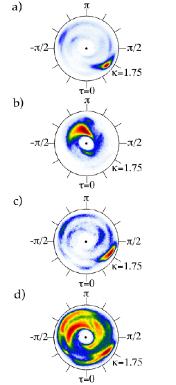
Figure 1: (Color online:) The four major protein structures: a) $\alpha$-helices, b) $\beta$-strands, c) $3/10$-helices and d) loops. We define these structures according to their PDB classification in our 2.0 Ȧ data set. In each Figure the center of the annulus is the north-pole of the two-sphere that surrounds the observer at the position $i$. This is the direction where the next $C_{\alpha}$ is located. At this point the bond (latitude) angle $\kappa=0$. The bond angle measures distance from the center of the annulus so that the south pole where $\kappa=\pi$ corresponds to points at infinity on the plane. The torsion i.e. longitude angle $\tau\in[-\pi,\pi]$ increases by $2\pi$ when we go around the center of the annulus in counter-clockwise direction. The color coding in all our Figures increases from white to blue to green to yellow to red describes the relative number of conformations in PDB in a $\log$-squared scale. The intensity is proportional to the probability of the direction where the observer turns at the next $C_{\alpha}$ carbon.

The four maps in Figure 1 portray non-local features that are not available in conventional Ramachandran plots. Moreover, instead of a discontinuous toroidal square as in the case of the Ramachandran plots, the predominant feature in all of the present maps is that the PDB data is concentrated in a continuous annulus which is roughly between the circles $\kappa_{in}\approx 1$ and $\kappa_{out}\approx\pi/2$. The exterior of the annulus $\kappa>\kappa_{out}$ is an excluded region, it describes conformations that are subject to steric clashes. The interior $\kappa<\kappa_{in}$ is sterically allowed but practically excluded as long as proteins remain in the collapsed phase; The interior region becomes occupied when we cross the $\Theta$-point and proteins assume their unfolded conformations.

We notice that loops appear to have a slightly higher tendency to bend towards left i.e. $\tau<0$. We also note that in the Figures for $\alpha$, $\beta$ and $3/10$ the blue regions correspond to residues where the present hydrogen-bond based PDB classification is in a miss-match with the geometric structure that is commonly associated with these configurations. Moreover, the Figure reveals that the PDB data displays innuendos of various underlying reflection symmetries: In the Figure 1d (loops) there is a clearly visible mirror of the standard right-handed $\alpha$-helix region, located in the vicinity of the outer rim with $\kappa\approx 3/2$ and with torsion angle close to the value $\tau\approx-2\pi/3$. A helix in this regime would be left-handed and tighter than the standard $\alpha$-helix. There is also a clear mirror structure in the Figure 1b for $\beta$ strands, the standard region is $(\kappa,\tau)\approx(1,\pi)$ and its less populated mirror is located around $(\kappa,\tau)\approx(1,0)$. The mirror symmetry between the ensuing extended regions persists in the Figure 1d for loops. Finally, in the Figure 1d we observe a small elevated (yellow) region in the vicinity of $(\kappa,\tau)\approx(3/2,-\pi/3)$. This is the region of helices that are spatial left-handed mirror images of the standard $\alpha$-helices. There is also a (slightly) elevated (green) mirror of this region around $(\kappa,\tau)\approx(3/2,2\pi/3)$. This is like the $(\kappa,\tau)\approx(3/2\,,-2\pi/3)$ mirror of the standard right-handed $\alpha$ helices.

IV Side-Chain mapping

We can similarly visualize the geometry of side-chain atoms, as they are seen by our roller-coasting observer. This gives us local information on the given peptide unit. Now the results turn out to be isomorphic to those revealed by the standard Ramachandran plot. Moreover, this enables us to develop a visual complement to the existing rotamer libraries.

We assume that the observer is oriented according to the discrete Frenet framing that is determined by the transfer matrix (4) at each $C_{\alpha}$. At the location of the $C_{\alpha}$ the observer then looks at the side-chain atoms and records the direction of each of them as points on the surface of the two-sphere that surrounds the observer, with the north-pole of the sphere always coinciding with the direction towards the next $C_{\alpha}$ exactly as in the case of the backbone.

In Figure 2 (top) we display the angular distribution of the $C_{\beta}$ carbons on the surface of the two-sphere for all the $C_{\alpha}$ carbons, as recorded by our Frenet frame observer who is located at the origin of the sphere. Recall that a $C_{\beta}$ carbon is present in all non-glycyl residues. We note that our framing is determined entirely in terms of the backbone. According to prevailing paradigm the directions of the $C_{\beta}$ carbons should then be directly computable from the geometry of the tetrahedral covalent bond structure of the pertinent $C_{\alpha}$ carbon. However, Figure 2 (top) reveals that the directions of the $C_{\beta}$ carbons are not determined only by the local covalent bond structure. In addition, these directions are clearly subject to secondary structure dependent but amino acid independent nutations. This confirms that at the level of accuracy of our data, the stereochemical restraints fail to be fully universal. They reflect the secondary structure environment sch -mart . In fact, despite being based entirely on the C_β atoms the Figure 2 is fully isomorphic to the standard Ramachandran plot, for all amino acids except for glycine that has no C_β.

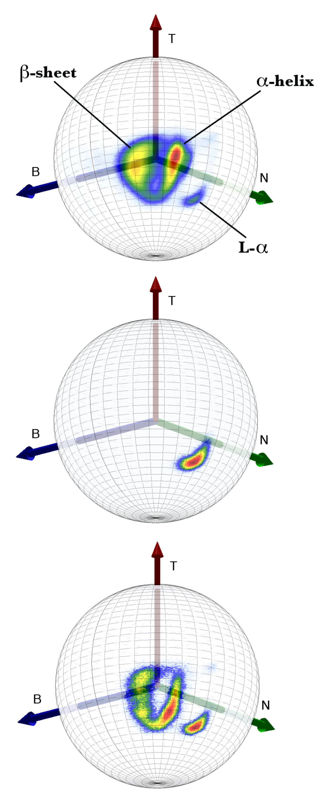
Figure 2: (Color online:) The directions of the $C_{\beta}$ carbons, as seen by our Frenet frame observer who is located at the corresponding $C_{\alpha}$ carbon which is at the center of the sphere. The vector $\mathbf{t}$ points to the direction of the next $C_{\alpha}$ carbon. On top all residues in our data set including ASN. In the middle we display only the $\tt L$-$\alpha$ region of the Ramachandran plot. On bottom we display only those ASN that are in a loop in PDB classification.

A important feature of the nutation is the presence of the highly localized, isolated island denoted $\tt L$-$\alpha$ that is clearly visible in Figure 2 (top). We have confirmed that this isolated island coincides exactly with the conventional non-glycyl $\tt L$-$\alpha$ region of the standard Ramachandran plot. This is shown in Figure 2 (middle) where we display the direction of the $C_{\beta}$ carbons solely for those non-glycyl residues that are in the $\tt L$-$\alpha$ Ramachandran region. Finally, in the Figure 2 (bottom) we display the discrete Frenet frame distribution of the $C_{\beta}$ carbons for those ASN that are located in loops only, according to PDB classification. The relatively high propensity of ASN in the $\tt L$-$\alpha$ island is prominent.

In the sequel we shall concentrate our attention solely on the isolated $\tt L$-$\alpha$ island in Figure 2 (middle). We start by noting the propensity of different amino acids in the $\tt L$-$\alpha$ island. The result (in percent) is shown in Figure 3. This Figure confirms the high propensity of ASN (N) that is also visible from Figure 2 (bottom). We find that ASP (D) has also relatively high relative propensity. But the propensity of histidine (H) is practically equal. Furthermore, several non-carbonylic amino acids have a higher propensity than GLU (E). Finally, the $\beta$-branched isoleucine (I), valine (V) and threorine (T) all have clearly suppressed propensities and proline (P) is practically absent, presumably reflecting the presence of steric constraints deane , review .

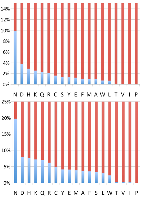
Figure 3: (Color online:) The percent distribution of non-glycyl residues in the $\tt L$-$\alpha$ island of Figure 2. In the top Figure we display the result for all amino acids in our entire data set, and in the bottom Figure for those in our data set that are classified as loops in PDB. The propensity of carbonylic ASN (N) is clearly enhanced in both cases. But in both cases the similarly carbonylic ASP (D) has about the same percent-wise propensity with the non-carbonylic HIS (H), and the carbonylic GLU (E) is relatively quite suppressed.

We now proceed to map the directions of the $C_{\gamma}$ carbons for those side-chains where $C_{\beta}$ is located in the $\tt L$-$\alpha$ island of Figure 2. We continue to utilize the framing determined by our observer who roller-coasts the $C_{\alpha}$ backbone with orientation determined by the discrete Frenet frames, and north-pole always in the direction of the next C_α. The result is presented in Figure 4. It reveals that at the level of $C_{\gamma}$, the single $\tt L$-$\alpha$ island of the $C_{\beta}$ becomes divided into two separate but still highly localized islands. This reflects the sp3 hybridization of the C_β: There is a putative gauche- ($g$-) island where around 70$\%$ of the residues in the $\tt L$-$\alpha$ island are located, and a putative trans island for the rest. Interestingly, we do not really see any putative gauche$+$ ($g+$) island.

The amino acid propensities of these two islands is displayed in Figure 5. ASN is the most populous in both $C_{\gamma}$ islands. However, the propensity of ASP is elevated only in trans island. In the g- island both non-carbonylic HIS (H) and LYS (K) and even the carbonylic GLN (Q) have a higher propensity than ASP. At the moment we have no good explanation for this observation, and we leave it as challenge.

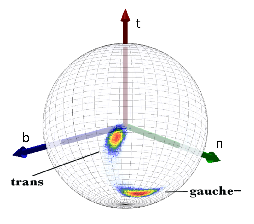
Figure 4: (Color online:) The directions of those $C_{\gamma}$ carbons for which the $C_{\beta}$ is located in the $\tt L$-$\alpha$ island, and as seen by our Frenet frame observer who is located at the $C_{\alpha}$ carbon which is situated at the center of the sphere.

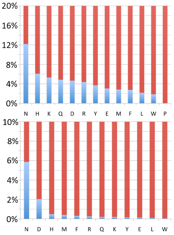
Figure 5: (Color online:) The percent-wise propensity of different amino acids in the putative g- island (top) and trans $C_{\gamma}$-island (bottom) in Figure 4

In Figure 6 we plot the percentage ratios of the different amino acids as they appear in the two $C_{\gamma}$ islands. We note that around $43\%$ of residues in the putative $\it g-$ island are non-carbonylic, while in the putative $\it trans$ island the number is much lower, close to $12\%$.

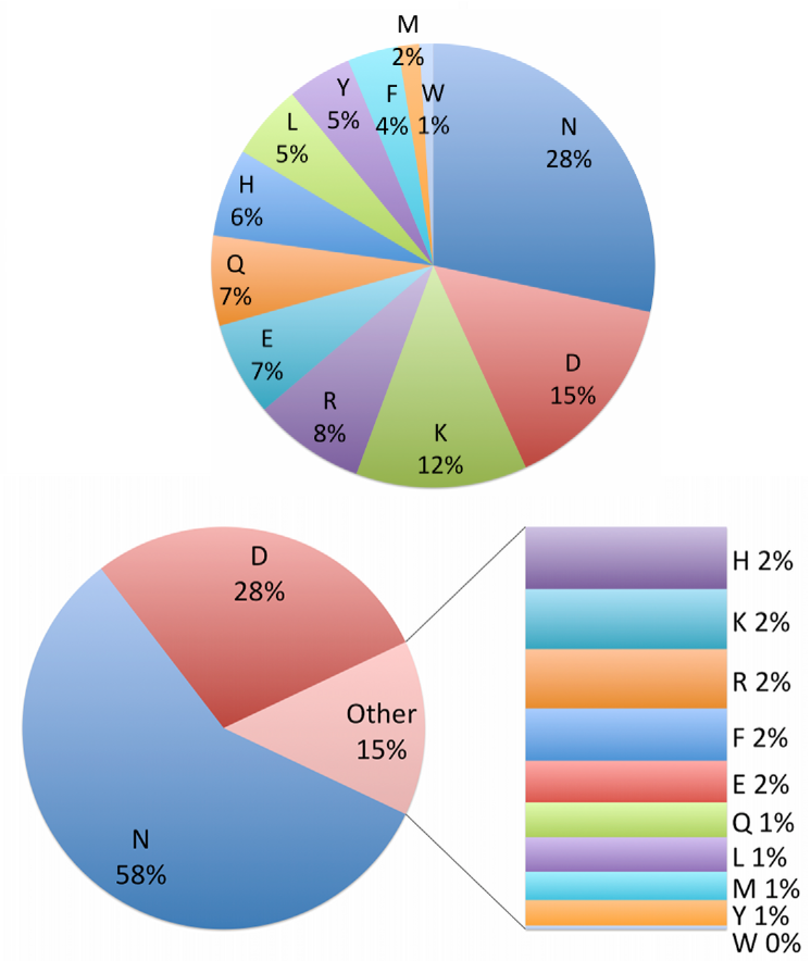
Figure 6: (Color online:) The relative number of different amino acids in the putative $\it g-$ (top) and $\it trans$ (bottom) $C_{\gamma}$-islands.

We proceed to the next level along the side-chain, to map the $C_{\delta}$ carbons. in Figure 7 we plot these carbons for those side-chains where $C_{\beta}$ is located in the $\tt L$-$\alpha$ island. In the Figure 7 on top, we show them as they are seen by by our discrete Frenet frame observer who sits at the locations of the $C_{\alpha}$ carbons. In the Figure 7 on bottom we show them as they are seen in the C_β frame for an observer now sitting at the C_β location, this time using the stereographic projection. Since ASN (and ASP) has no $C_{\delta}$ carbon, we display instead the direction of the side-chain $O$ atom for ASN, the result is shown in Figure 8. In the top Figure 8 we use the C_α based Frenet frame observer and in the middle and bottom Figure 8 we use the C_β frame observer in combinations with stereographic projection.

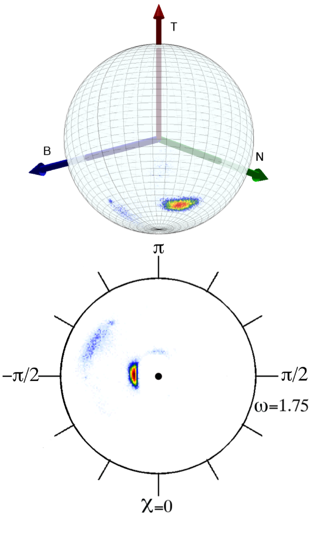
Figure 7: (Color online:) The directions of the $C_{\delta}$-carbons in the discrete Frenet frame of the $C_{\alpha}$ carbons on the surrounding two-sphere (top) and in the C_β frame (bottom). In the Figure on top, the C_β atom is located at the origin of the two-sphere, which is stereographically projected from the north pole (with C_α at the south pole).

From Figure 7 we observe that the directions of the $C_{\delta}$ continue to be highly localized, independently of the type of amino acid. But unlike in the case of $C_{\gamma}$, we find quite surprisingly, that now there is only one clearly visible island. We do not have any definite stereochemistry or physics based explanation why the clearly visible sp3 hybridization based doubling that we observe at the level of $C_{\gamma}$ has now completely disappeared. However, we do observe the formation of a second, relatively very weakly occupied island at larger values of the latitude angle and with longitude angle $\chi\sim-2\pi/3$. This island is clearly visible in Figure 7 (right). There is also a third, very faint island in the direction $\chi\sim\pi$ that (barely) becomes visible in the stereographically projected Figure 7 (left). At the moment we do not have a basis to conclude whether the extremely low population of the second and third island is a real effect or only a reflection of problems in the experimental data. We refer to errors , that there are presently an estimated half a million incorrectly positioned side-chain atoms PDB data. In this light, the reason for the sparse population of the two additional sp3 hybridized islands should be subjected to experimental curiosity, to determine the cause.

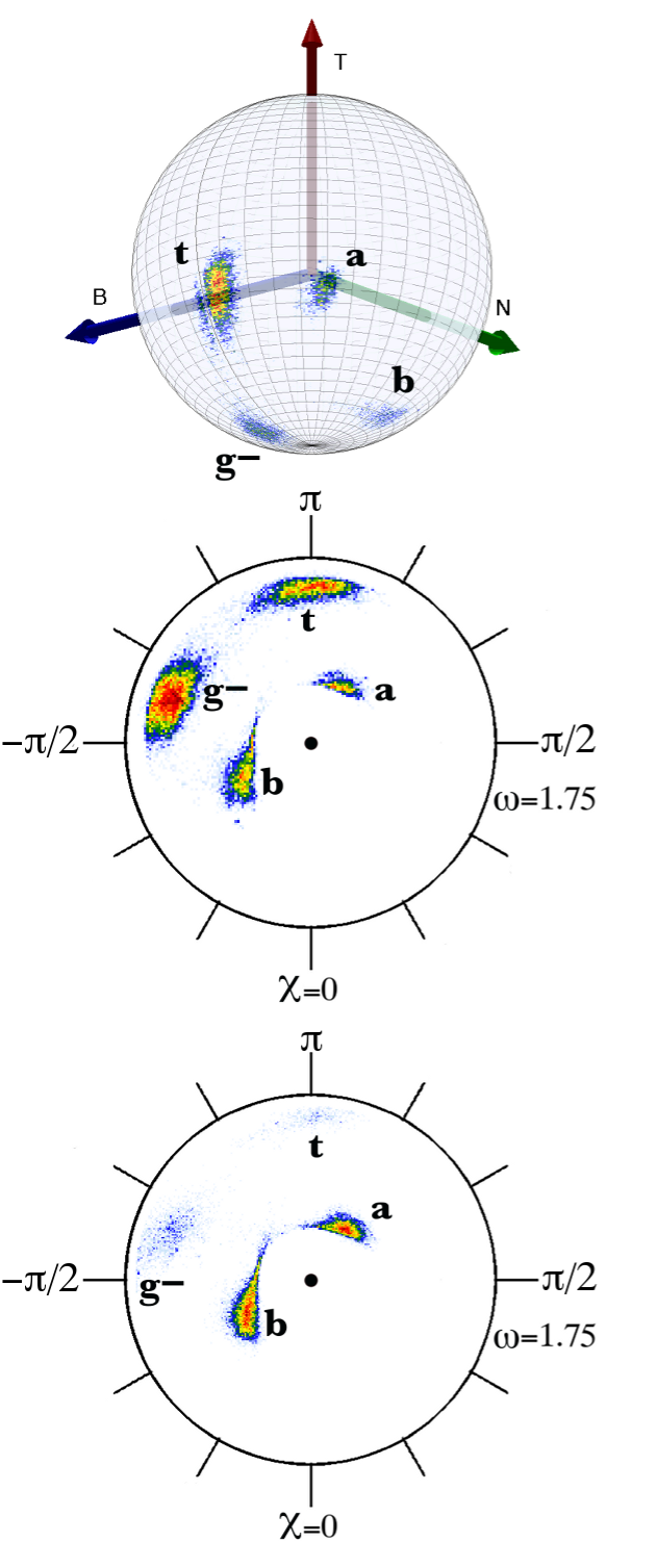
Figure 8: (Color online:) On top, the directions of the side-chain $O$ atoms of ASN in the discrete Frenet frame of the $C_{\alpha}$ carbons. In the middle and bottom we use the same stereographically projected C_β frames as in Figure 7 (right). The Figure in middle displays the same atoms as the Figure on top. On bottom, the directions of the side-chain $N$ atoms of ASN suggests that the correct identification of a and b regions in the top and middle figure should be $N$ and not $O$ as in PDB. Similarly, the regions t and g- in the bottom should be $O$ and not $N$ in PDB. See errors . (t is trans and g- is gauche-)

Since ASN has no $C_{\delta}$ carbon, in Figure 8 we display instead the $O$ atoms of the ASN side-chain according to PDB identification. In the top Figure 8 we use discrete Frenet frame of the $C_{\alpha}$-carbons, and in the middle and bottom we use the stereographically projected C_β frame. We note that the two $C_{\gamma}$ islands appear to become divided into four distinct but still highly localized islands. However, we recall that the identification between the ASN side-chain $O$ and $N$ can be very difficult, and there are apparently numerous errors in the $O$ and $N$ identifications in PDB data errors . Thus we have displayed in Figure 8 (top) the $N$ atoms according to PDB identification as well. By comparing the Figures 8 (middle) and (bottom) we propose that most likely the two inner-most islands denoted a and b in Figure 8 describe $N$ instead of $O$ atoms. If so, our visualization technique could become a useful tool in detecting erroneously identified $O$ and $N$ atoms and help to resolve the kind of issues raised in errors . This could be scrutinized by a careful re-analysis of high resolution x-ray crystallography data.

Finally, in Figure 9 we have mapped the locations of the C_γ atoms in our entire dataset (except for prolines) as they are seen in the stereo graphically projected C$-\beta$ frame. In the Figure at top we show all atoms except those that have C_β in the $\tt L$-$\alpha$, and in Figure at bottom we show only the $\tt L$-$\alpha$ atoms. The sp3 hybridization of the C_β covalent bond structure is clearly visible. Furthermore, in each of the three regions in left we recognize the substructure that correspond to the $\alpha$-helices, $\beta$-strands and the interconnecting loops. Each of the three regions is then isomorphic to Figure 2a.

Obviously, it is straightforward to continue the present analysis to inspect additional side-chain atoms. However, here our goal is not to perform a detailed and complete analysis of all the side-chain atoms, we simply aim to describe a method.

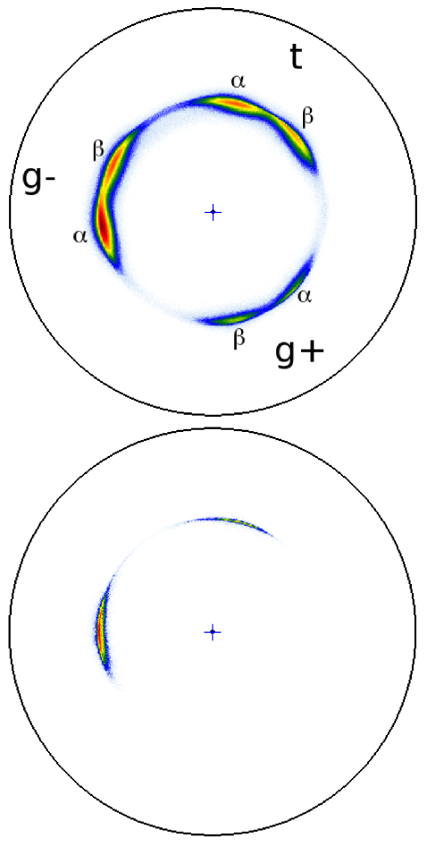
Figure 9: (Color online:) The directions of the C_γ atoms in the C_β centered frames, on two-sphere stereographically projected from its north pole and with C_α at south-pole. On the top all those C_γ atoms for which the C_β is not in the $\tt L$-$\alpha$, and on bottom those that correspond to C_β in the $\tt L$-$\alpha$ island. (gauche- on left, t on top-right and gauche+ on bottom-right.)

V solitons

The localization we have observed in the $\tt L$-$\alpha$ side-chain atoms proposes that there is an organizational principle in the side-chain orientations that extends beyond a single peptide unit. Hence it can not be detected by the Ramachandran plot or in terms of the standard rotamer libraries, these only provide information on a given peptide unit. The backbone C_α atoms we have inspected all correspond to the $\tt L$-$\alpha$ position of the C_β, this region is known to commonly appear in connection of loops in lieu of regular secondary structures. Thus the order we have observed is a priori not a reflection of any apparently regular secondary structure category at the level of the backbone geometry, but a characteristic of loops. We propose that it is due to the presence of a soliton solution to a discrete version of nonlinear Schrödinger (DNLS) equation that universally describes the backbone C_α geometry in (practically) all folded proteins.

For the soliton description we do not need to know the atomic level details of the energy function. We only need to apply general symmetry principles to the abstract full quantum mechanical, all-atom Hamiltonian operator $\mathcal{H}[q_{i},p_{i}]$. Here the index i = 1, …, N labels all pairs of canonical coordinates $(q_{i},p_{i})$ that describe the elementary constituents. These include the individual C, O, N, H and every other atom in the protein and in the solvent. We also account for the valence electrons, and for every local and long range interaction between all the atoms both in the protein and in the solvent. For simplicity we take all the variables to be point-like, that is we work at the first quantized level. The canonical partition function is computed by the path integral,

$$\mathcal{Z}=Tre^{-\beta\mathcal{H}}=\int[dq]e^{-\frac{1}{\hbar}\mathcal{S}(q,\dot{q})}$$

where $\mathcal{S}(q,\dot{q})$ is the classical Euclidean action of $\mathcal{H}[q_{i},p_{i}]$. The integration extends over all period configurations (anti-periodic in the case of fermions). With the partition function we obtain the thermodynamical Helmholtz free energy as follows: We introduce external sources $j_{i}(t)$ and extend the partition function into the generating functional of connected Green’s functions,

$$W[j]=\ln\left\{\int[dq]e^{-\frac{1}{\hbar}\mathcal{S}_{\beta}+\frac{1}{\hbar}\int\limits_{0}^{\hbar}\beta j\dot{q}}\right\}$$

We introduce the Legendre transformation

$$\Gamma[q]=-\frac{1}{\beta}\left\{W[j]-\int\limits_{0}^{\hbar\beta}\frac{\delta W}{\delta j}\cdot j\right\}$$

This defines the effective action that coincides with the Helmholtz free energy when we take the limit $j_{i}\to 0$.

There are various methods to compute the Helmholtz free energy $E$. Here we introduce a finite difference version of the gradient expansion. In the leading nontrivial order we have

$$E=\lim\limits_{j_{i}\to 0}\Gamma[q]=\sum_{i}V^{(i)}(q_{i})+F^{(i)}(q_{i},q_{i+1})+\dots$$

$$=\sum_{i}V^{(i)}(q_{i})+\frac{\partial F^{(i)}(q_{i},q_{i+1})}{{\partial q_{i+1}}_{|q_{i+1}=0}}q_{i+1}\ +\dots$$ (7)

The potentials $V^{(i)}$ are all local and the $F^{(i)}$ are bi-local. The higher order terms in the expansion are either higher order polynomials in the nearest neighbor variables, or terms that introduce couplings between next-to-nearest neighbor variables.

In the expansion (7), in the case of the backbone we identify the generalized coordinates $q_{i}$ with the bond and torsion angles ($\kappa_{i},\tau_{i}$) in (2), (3). We assume that all the additional variables that appear in the full Hamiltonian operator $\mathcal{H}[q_{i},p_{i}]$ have been integrated over in constructing the partition function. They affect the detailed functional form of the coefficients $V^{(i)}$, $F^{(i)}$ etc. in (7). Since (5) contains only the $\mathbf{t}_{i}$, it is clear that the expansion (7) in terms of ($\kappa_{i},\tau_{i}$) must remain invariant if we introduce a local frame rotation in the normal plane spanned by ($\mathbf{n}_{i},\mathbf{b}_{i}$). This introduces a strong constraint to its functional form. In oma1 , ulf this has been utilized to show that in the leading order the expansion (7) is uniquely determined. It can only contain the following terms cherno -peng , ulf ,

$$E=-\sum\limits_{i=1}^{N-1}2\,\kappa_{i+1}\kappa_{i}+\sum\limits_{i=1}^{N}\left\{2\kappa_{i}^{2}+q\cdot(\kappa_{i}^{2}-m^{2})^{2}\right.$$

$$\left.+\frac{d_{\tau}}{2}\,\kappa_{i}^{2}\tau_{i}^{2}-b_{\tau}\kappa_{i}^{2}\tau_{i}-a_{\tau}\tau_{i}+\frac{c_{\tau}}{2}\tau^{2}_{i}\right\}$$ (8)

Here the first sum together with the three first terms in the second sum coincide with the integrable energy function of the conventional DNLS equation with a potential that displays spontaneous symmetry breaking. The fourth ($b_{\tau}$) and the fifth ($a_{\tau}$) terms are the only two lower order nontrivial conserved quantities that appear in the integrable DNLS hierarchy prior to the energy. These are the momentum and the helicity, respectively. The last ($c_{\tau}$) term is the standard Proca mass term. The parameters are all global and specific only to a super-secondary structure such as helix-loop-helix. In particular they are independent of the detailed nature of amino acids.

Unlike a force field in molecular dynamics, the energy function (8) does not describe the fine details of the atomary level interactions such as Coulomb, van der Waals, hydrogen bonding etc. Instead, like an effective Landau-Lifschitz theory it describes the properties of a folded protein backbone in terms of universal physical arguments. Full details and motivation of (8) are presented in cherno -peng , ulf

The remarkable property of (8) is that the torsion angle $\tau_{i}$ is only subject to local interactions, all explicit non-local interactions are carried by the bond angle $\kappa_{i}$. Furthermore, since $\tau_{i}$ appears at most quadratically we can solve for it in terms of $\kappa_{i}$,

$$\tau_{i}=\frac{a_{\tau}+b_{\tau}\kappa_{i}^{2}}{c_{\tau}+d_{\tau}\kappa_{i}^{2}}$$ (9)

When we substitute this into the variational equation of $\kappa_{i}$ that follows from (8), we arrive at a generalized version of the DNLS equation. Its soliton solution has been constructed in cherno -peng . In particular, it has been observed that the soliton can be approximated by the discretized version of the soliton solution of the continuum dark NLSE soliton davy -fadd ,

$$\kappa_{i}=\frac{m_{1}\cdot e^{c_{1}(i-s)}-m_{2}\cdot e^{-c_{2}(i-s)}}{e^{c_{1}(i-s)}+e^{-c_{2}(i-s)}}$$ (10)

Here the various parameters each have a natural interpretations, see cherno -peng for a detailed description: The parameter $s$ determines the backbone site location of the center of the fundamental loop that is described by the soliton. The values of the parameters $m_{1,2}\in[0,\pi]\ mod(2\pi)$ are entirely determined by the bond angles of the adjacent helices and strands. Finally, only the $c_{1}$ and $c_{2}$ are intrinsically loop specific parameters, they specify the length of the loop. The soliton profile of $\kappa_{i}$ determines the torsion angles $\tau_{i}$ by (9). According to peng practically all PDB proteins can be constructed as the sum of terms of the form (10), in a modular fashion from a relatively small number of soliton profiles.

Following mart we argue that in the Frenet frames, the angular positions of the side-chain atoms can be similarly determined in terms of the corresponding $\kappa_{i}$ values only. For this we denote by ($\theta,\phi$) the standard spherical latitude and longitude angles of the sphere that surrounds the C_α observer. We propose that to leading order in the expansion (7), in these coordinates each of the side-chain atoms has an energy function that has the same functional form as the energy function of the backbone torsion angles. Consequently, for each side-chain atom we introduce only the following two leading contributions to the energy

$$E_{\theta}=\sum\limits_{i=1}^{N}\left\{\frac{d_{\theta}}{2}\,\kappa_{i}^{2}\theta_{i}^{2}-b_{\theta}\kappa_{i}^{2}\theta_{i}-a_{\theta}\theta_{i}+\frac{c_{\theta}}{2}\theta^{2}_{i}\right\}$$ (11)

$$E_{\varphi}=\sum\limits_{i=1}^{N}\left\{\frac{d_{\varphi}}{2}\,\kappa_{i}^{2}\varphi_{i}^{2}-b_{\varphi}\kappa_{i}^{2}\varphi_{i}-a_{\varphi}\varphi_{i}+\frac{c_{\varphi}}{2}\varphi^{2}_{i}\right\}$$ (12)

Note that these contributions have been carefully selected so that they will not change the functional form of(8). The addition of (11), (12) will only redefine the coefficients in the $\kappa_{i}$ dependent terms in (8) which does not lead to any change in the underlying soliton structure. In particular, we can still utilize the approximative soliton profile (10). In parallel with (9) the spherical angles ($\theta_{i},\varphi_{i}$) for each of the side-chain atoms are then dynamically determined by the DNLS soliton profile of the backbone bond angles $\kappa_{i}$,

$$\theta_{i}=\frac{a_{\theta}+b_{\theta}\kappa_{i}^{2}}{c_{\theta}+d_{\theta}\kappa_{i}^{2}}$$

$$\varphi_{i}=\frac{a_{\varphi}+b_{\varphi}\kappa_{i}^{2}}{c_{\varphi}+d_{\varphi}\kappa_{i}^{2}}$$

The present visual analysis implies that in the case of a $\tt L$-$\alpha$ residue the numerical values of both ($b_{\theta},d_{\theta}$) and ($b_{\varphi},d_{\varphi}$) are vanishingly small for the C_β, C_γ and C_δ carbons, and for the side-chain $N$ and $O$ atoms in the case of ASN and ASP. But both ($a_{\theta},c_{\theta}$) and ($a_{\varphi},c_{\varphi}$) have amino acid independent, finite and universal values that can be directly inferred from the Figure 2 (middle), 4, 7 and 8 respectively,

$$<\theta_{i}>_{{\tt L}-\alpha}\ \approx\frac{a_{\theta}}{c_{\theta}}$$

$$<\varphi_{i}>_{{\tt L}-\alpha}\ \approx\frac{a_{\varphi}}{c_{\varphi}}$$

We now proceed to argue that these universal values can be understood in terms of relatively few DNLS solitons. We then show how these solitons can be classified using our graphical tools.

VI soliton visualization

It has been argued in the literature that in the case of ASN and ASP the $\tt L$-$\alpha$ Ramachandran region become stabilized by a local but non-covalent attractive interaction between the side-chain and backbone carbonyls, with the backbone oxygen atom in a special rôle deane , review . Unlike the Ramachandran plot, our Frenet framing can provide information on the neighboring peptide units and we have investigated the directions of all backbone $O$ atoms in our data set, in a group of residues around the $i^{th}$ side-chain $C_{\beta}$ that is located in the $\tt L$-$\alpha$ island. The result shown in Figure 10 displays how these $O$ atoms are seen by our Frenet frame observer who is located at the $i^{th}$ central $C_{\alpha}$ carbon. Our observer finds that the directions of the nearby backbone $O$ atoms are very srongly localized and correlated. The localization is residue independent and extends itself over at least four different residues:

$\bullet$ For the $i-2$ site there is strong localization with a three-fold degeneracy that is reminiscent of the trans/gauche (sp3 hybridization) degeneracy. The data is consistent with vanishing values of both ($b_{\theta},d_{\theta}$) and ($b_{\varphi},d_{\varphi}$).

$\bullet$ For the site $i-1$ we have very strong localization along the longitudinal ($\varphi_{i-1}$) direction, with a tiny oscillation in the latitudinal ($\theta_{i-1}$) direction. For the corresponding energy, ($b_{\varphi},d_{\varphi}$) are again vanishingly small while ($b_{\theta},d_{\theta}$) are now small but non-vanishing.

$\bullet$ For the site $i$ we have a single localized oscillator in the longitudinal direction. Thus ($b_{\varphi},d_{\varphi}$) are now small but non-vanishing while ($b_{\theta},d_{\theta}$) vanish.

$\bullet$ For the site $i+1$ we again find the three-fold trans/gauche degeneracy: There are three oscillators in the longitudinal direction, and they are all located very close to the north-pole. Consequently ($b_{\theta},d_{\theta}$) vanish while ($b_{\varphi},d_{\varphi}$) do not. In fact, the $\varphi_{i+1}$ amplitudes are quite large.

The localization pattern of the backbone $O$ atoms means that for our Frenet frame observer the backbone geometry around a $\tt L$-$\alpha$ residue shows very little variations. Only a very limited set of extended backbone geometries are accessible. Since the regime that covers the sites from the $(i-2)^{th}$ to the $(i+1)^{th}$ involves four sets of bond and torsion angles, each of them defined in terms of three resp. four residues we conclude that the geometries reflect the non-local collective interplay of at least up to seven different residue sites along the backbone. This is in line with our proposal that the positions of the side-chain atoms are determined dynamically by the backbone, in terms of a small number of different DNLS soliton profiles according to (11), (12).

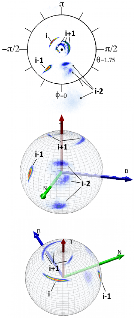
Figure 10: (Color online:) The orientations of backbone $O$ atoms around the site $i$ that is located in the $\tt L$-$\alpha$ island, as seen by our discrete Frenet frame observer at the $i^{th}$ central $C_{\alpha}$-carbon, on a stereographically projected two-sphere (top) and on the surrounding two-sphere that we have displayed from two different perspectives (middle, bottom). For the $i^{th}$ and $(i-1)^{th}$ atom only one position appears to be available while the $(i+1)^{th}$ and $(1-2)^{th}$ atoms each have three available (trans/gauche) positions. The angle $\phi$ is measured from the $\bf N$ axis.

To expose the soliton structures that surround the $\tt L$-$\alpha$ island, we consider the distribution of the backbone bond and torsion angles that are attached to those $C_{\alpha}$ carbons where the $C_{\beta}$ atom is in the $\tt L$-$\alpha$ position. The result is shown in Figure 11 on a stereographically projected two-sphere, separately for ASN and ASP and for the remaining non-glycyl amino acids.

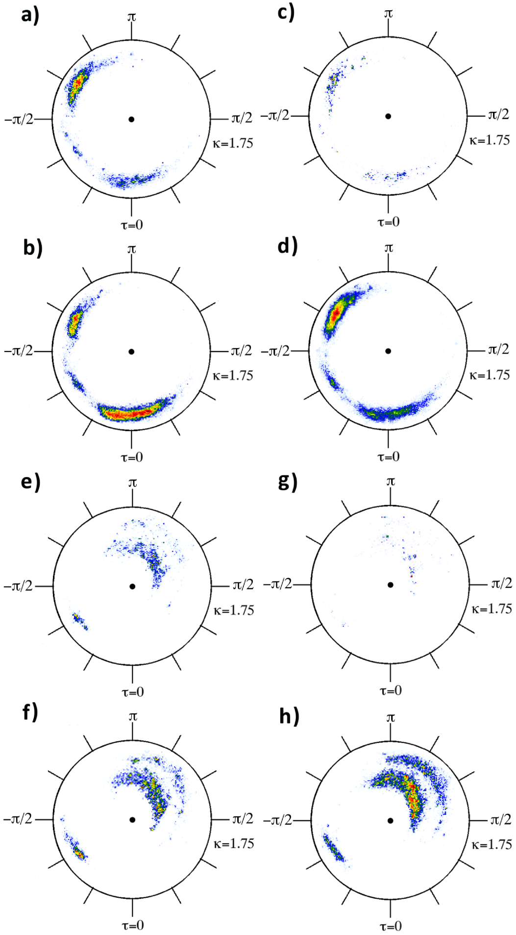
Figure 11: (Color online:) The $(\kappa,\tau)$ distributions for backbone links that are attached to a $C_{\alpha}$ carbon with $C_{\beta}$ in the $\tt L$-$\alpha$ island on stereographically projected two-sphere as in Figure 1. We display separately ASN, ASP, and all the rest. On left column the $C_{\alpha}$ carbons in the case where the corresponding $C_{\gamma}$ carbon is in the trans island, on right for those where the $C_{\gamma}$ is in the $g$- island. First row a),c) is for link that precedes either ASN or ASP. Second row b),d) is for link preceding any other non-glycyl amino acid. Third row e),g) is for link following either ASN or ASP. Fourth row f),h) is for link following the others.

We observe no practical difference between the residues. Nor do we find any practical difference between the various trans and $g$- positions. Instead, we do observe the following general pattern: For the backbone $C_{\alpha}$-$C_{\alpha}$ link that precedes the $\tt L$-$\alpha$ island, three different regions on the $(\kappa,\tau)$ plane are probable. These are the regions that we have denoted with a, b and c respectively in the Figure 12 (top); In this Figure we have combined all the data that are displayed separately in the parts a, b, c and d of Figure 11. After the $\tt L$-$\alpha$ island there are also three different regions that are probable. We denote these regions with letters b and d and e respectively in the Figure 12 (bottom), now combining the data in parts e, f, g, h in Figure 11. Note that the regions b in the two parts of Figure 12 practically overlap.

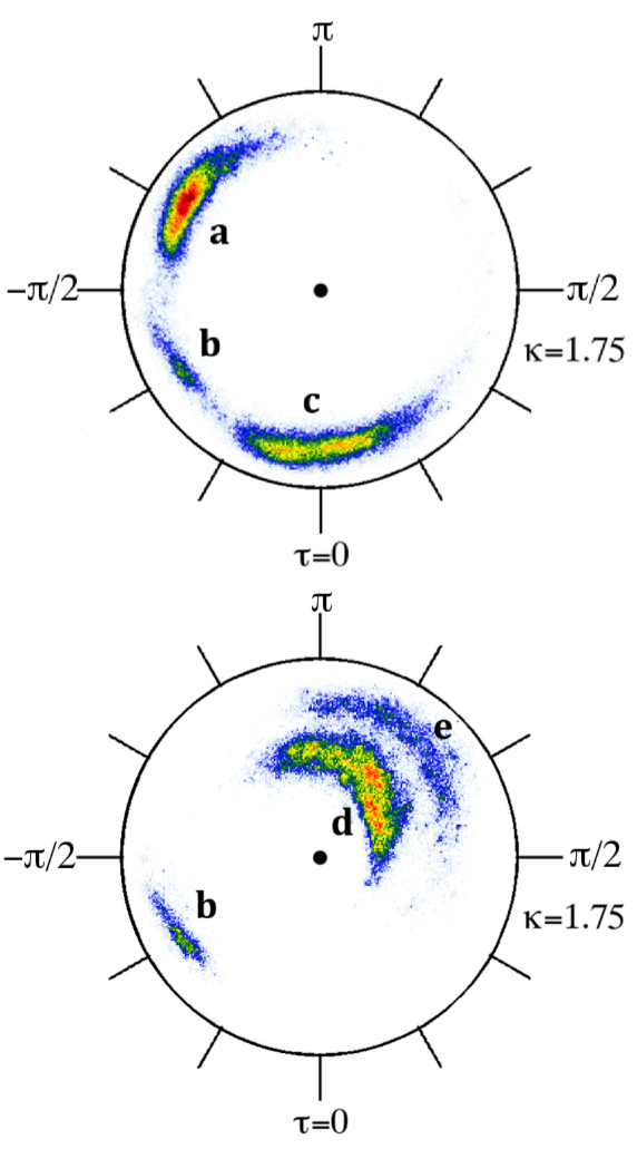
Figure 12: (Color online:) The $(\kappa,\tau)$ distributions for all backbone links that are attached to a residue in the $\tt L$-$\alpha$ island. On the top for the link preceding the residue in the $\tt L$-$\alpha$ island, on the bottom following the residue in the $\tt L$-$\alpha$ island.

By inspecting the protein structures in our data set we conclude that the presence of a residue in the $\tt L$-$\alpha$ island causes the following phenomenological selection rules between the regions displayed in Figure 12. When we roller-coast along the backbone:

$\bullet$ The region a can only precede regions d and e.

$\bullet$ Both regions b and c can be followed by any of the three regions b, d and e.

$\bullet$ The residue preceding either a or c is not located in the $\tt L$-$\alpha$ island.

$\bullet$ Both the residue preceding and following b can be located in the $\tt L$-$\alpha$ island.

$\bullet$ If the two residues following c are both in the $\tt L$-$\alpha$ island, the first residue connects c to b and the second connects b to b.

These are the selection rules, that limit the available global topology of the backbone solitons when we pass the $\tt L$-$\alpha$ site. Notice that since the region b has the same bond angle as the standard $\alpha$-helix region and since the torsion angles are equal in magnitude but have an opposite sign, a repeated structure in b is the right-handed mirror image of the standard $\alpha$-helix. Consequently this is truly the region of left-handed $\alpha$-helices.

These selection rules classify the different possible DNLS soliton profiles in the presence of the $\tt L$-$\alpha$ island. In particular, we have found that there seems to be no more than four solitons that are particularly common around a residue with $C_{\beta}$ located in the $\tt L$-$\alpha$ island. We now describe these solitons qualitatively using our visual tools, as transition trajectories between the different regions that appear in the maps of Figure 1. These transitions illustrate how our observer turns at the location of each $C_{\alpha}$ as she roller-coasts through the soliton. The results are shown in Figure 13. In each case the pink arrow corresponds to a site where $C_{\beta}$ is located in the $\tt L$-$\alpha$ island; Recall that the bond and torsion angles are link variables, they connect two $C_{\alpha}$ carbons according to (4). Clearly, the Figure 13 is but an example of a general method to visually classify solitons in a manner that directly reflects the geometry of the underlying backbone.

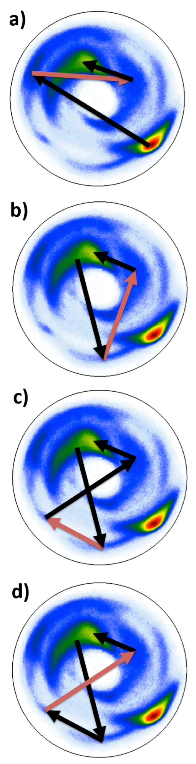
Figure 13: (Color online:) Four different soliton trajectories through a residue in the $\tt L$-$\alpha$ island that are common in our data set, on the stereographically projected two-sphere. The arrow shows how the Frenet frame observed sees the soliton to proceed from a $C_{\alpha}$ to the next $C_{\alpha}$. In each case the pink line denotes the transition that is caused by the presence of a residue in the $\tt L$-$\alpha$ island. The trajectory a described a soliton that connects the $\alpha$-helix region to the $\beta$-strand region. The remaining ones all both start and end in the $\beta$-strand region.

$\bullet$ In Figure 13a, the first residue takes our observer away from an $\alpha$-helix region to the region a in the Figure 12 left (black arrow). This is followed by a residue in the $\tt L$-$\alpha$ island, that takes the observer to the region d in the Figure 12 right (pink arrow). Finally, there is a transition to the $\beta$-strand region (black arrow). Consequently this is a short soliton that takes us from the ground state which is an $\alpha$-helix to the other ground state which is a $\beta$-strand.

$\bullet$ The second soliton trajectory shown in Figure 13b starts from the $\beta$-strand region with a residue that takes the observer into region c in Figure 12 left. The following residue that is located in the $\tt L$-$\alpha$ island then causes a transition into region d in Figure 12 right (pink arrow). This is followed by a transition back to a $\beta$-strand region. Since the initial and final positions are in a $\beta$-strand, this is an example of a soliton that combines the $\beta$-strand with another $\beta$-strand.

$\bullet$ The third trajectory that we have described in Figure 13c starts from the $\beta$-strand region and proceeds to region c in Figure 12 left. From there the trajectory proceeds to region b in Figure 12 left, with the transition caused by a residue in the $\tt L$-$\alpha$ island. This is followed by a transition to region d and then back to the $\beta$-strand region. This trajectory is also an example of a soliton that combines the $\beta$-strand with another $\beta$-strand.

$\bullet$ Finally, the fourth trajectory that is also common in our data set is the one displayed in Figure 13d. It is similar with the trajectory described in Figure 13c, except that now the residue that is located in $\tt L$-$\alpha$ island causes the transition from b to d in Figure 12. This trajectory is also an example of a soliton that combines the $\beta$-strand with another $\beta$-strand.

The remarkable property of solitons c) and d) in Figure 13 is, that they have similar overall topology and differ from each other only by the location of the $\tt L$-$\alpha$ along the trajectory. It is quite plausible that in some proteins these two solitons are but two states of an oscillating discrete ”breather” soliton. The ensuing proteins are presumable unstructured.

Finally, for the purposes of soliton taxonomy we note that when we analyze the proteins in the version v3.3 Library of chopped PDB files for representative CATH domains we find that the propensity of our solitons is largest in the (mainly-$\beta$) CA level classes 2.90, 2.160 where over 5$\%$ of all residues are in the $\tt L$-$\alpha$ island. We also find that any CA level family has at least 1$\%$ of their residues in the island, except 1.40 where the single representative with PDB code 1PPR has no residues in the island.

VII Conclusion

We have developed a new visualization method of proteins. In the case of backbones our method provides information about the geometry of neighboring peptide units. This enables us to go beyond the regime of the canonical Ramachandran plot which does not contain information on the neighboring units. As an example of side chains, we have visually investigated the non-glycyl residues that are located in the $\tt L$-$\alpha$ region of the Ramachandran plot. Independently of the amino acid, we find that for a discrete Frenet frame observer who roller-coasts along the backbone $C_{\alpha}$ carbons the corresponding side-chain $C_{\beta}$ carbons are always localized in the same direction which is clearly different from the direction of the $C_{\beta}$ carbons in the right-handed region. This universality in the orientation persists when we investigate the $C_{\gamma}$ and $C_{\delta}$ carbons, and the side chain $O$ and $N$ atom in the case of ASN and ASP. The results suggest that instead of reflecting only a local interaction between a given backbone unit and its residue, the $\tt L$-$\alpha$ island is also associated with a largely residue independent backbone conformation.

When we proceed to analyze the distribution of those backbone bond and torsion angles that are associated with the links that both precede and follow a residue that is located in the $\tt L$-$\alpha$ island, we find that independently of the residue these angles display very similar patterns. Since the definition of a bond angle takes three $C_{\alpha}$ carbons and the definition of a torsion angle takes four, this prompts us to propose that the geometrical structure associated with the presence of a residue in the $\tt L$-$\alpha$ island is a soliton that reflects the interplay of at least seven consecutive backbone units. In particular, we have not been able to pin-point any obvious local reason (charged, polar, acidic, hydrophobic/philic) to explain the presence or absence of a residue on the $\tt L$-$\alpha$ region.

Our approach is based on a novel visualization method to depict proteins. This method is based on advances in three dimensional visualization techniques that have been developed after Ramachandran presented his plot. In the course of our analysis we have been able to observe several systematic patterns including potential anomalies in the PDB data. The visualization method we have developed shows promise to become a valuable tool for both experimental and theoretical protein structure analysis and fold description, in particular for visually describing and classifying the backbone solitons and as a complement to existing side-chain rotamer libraries.

References

- (1) G. Ramachandran, C. Ramakrishnan and V. Sasisekharan, Journ. Mol. Biol. 7 95 (1963)
- (2) C. Ramakrishnan and G. Ramachandran, Biophys. J. 5 909 (1965)
- (3) J. Janin, S. Wodak, M. Levitt, D. Maigret, J Mol Biol. 125 357 (1978)
- (4) A.J. Hanson, Visualizing Quaternions, Morgan Kaufmann Elsevier (London, 2006)
- (5) J.B. Kuipers, Quaternions and Rotation Sequences: a Primer with Applications to Orbits, Aerospace, and Virtual Reality, Princeton University Press (Princeton, 1999)
- (6) M.N.Chernodub, S. Hu and A.J. Niemi Phys. Rev. E82 011916 (2010)
- (7) N.Molkenthin, S. Hu and A.J. Niemi Phys. Rev. Lett. 106 078102 (2011)
- (8) A. Krokhotin, A.J. Niemi and X. Peng, arXiv:1109.3903v1 [physics.bio-ph]
- (9) A.S. Davydov, Journ. Theor. Biol. 66 379 (1977)
- (10) P.G. Kevrekidis, The Discrete Nonlinear Schr dinger Equation: Mathematical Analysis, Numerical Computations and Physical Perspectives (Springer-Verlag, Berlin, 2009)
- (11) L.D. Faddeev and L.A. Takhtajan, Hamiltonian methods in the theory of solitons (Springer Verlag, Berlin, 1987)
- (12) S.Hu, M. Lundgren and A.J. Niemi Phys. Rev. E83 061908 (2011)
- (13) C.M. Deane, F.H. Allen, R. Taylor and T.L. Blundell, Prot. Eng. 12 1025 (1999)
- (14) F.H. Allen, C.A. Baalham, J.O.M. Lommerse and P.R. Raithby, Acta Crystallog. B54 320 (1998)
- (15) P. Chakrabarti and D. Pal, Prog. Biophys. Molec. Biol. 76 1 (2001)
- (16) N.E. Robinson and A.B. Robinson, PNAS (USA) 98 12409 (2001)
- (17) C.R. McCuddena and V.B. Kraus, Clinic. Biochem. 39 1112 (2006)
- (18) N.E. Robinson and A.B. Robinson, Molecular Clocks Deamidation of Asparaginyl and Glutaminyl Residues in Peptides and Proteins Althouse Press (London, 2004)
- (19) E.H. Koo, P.T. Lansbury and J.W. Kelly, PNAS (USA) 96 9989 (1999)
- (20) R.L. Bishop, Am. Math. Monthly 82 246-251 (1974)
- (21) R.S. Hartenberg and J. Denavit, Kinematic synthesis of linkages McGraw-Hill (New York, NY, 1964)
- (22) H.M. Berman, K. Henrick, H. Nakamura and J.L. Markley, Nucl. Acids Res. 35 (Database issue) D301 (2007)
- (23) C.A. Orengo, A.D. Michie, S. Jones, D.T. Jones, M.B. Swindells and J.M. Thornton, Structure 5 1093 (1997)
- (24) L. Schäfer and L.M. Cao, Journ. Mol. Struc. 333 201 (1995)
- (25) P.A. Karplus, Prot. Sci. 5 1406 (1996)
- (26) D.S. Berkholz, M.V. Shapovalov, R.L. Dunbrack, Jr. and P.A. Karplus, Structure 17 1316 (2009)
- (27) W.G. Touw and G. Vriend, Acta Cryst. D66 1341 (2010)
- (28) M. Lundgren and A.J. Niemi, arXiv:1109.0423v1 [q-bio.BM]
- (29) C.X. Weichenberger and M.J. Sippl, Nucl. Acids Res. 35 (Web Server Issue) W403 (2007)
- (30) A.J. Niemi, Phys. Rev. D67 106004 (2003)
- (31) U.H. Danielsson, M Lundgren and A.J. Niemi, Phys. Rev. E82 021910 (2010)