Hadronic effects in low–energy QCD: inclusive $\tau$ lepton decay

Abstract

The inclusive $\tau$ lepton hadronic decay is studied within Dispersive approach to QCD. The significance of effects due to hadronization is convincingly demonstrated. The approach on hand proves to be capable of describing experimental data on $\tau$ lepton hadronic decay in vector and axial–vector channels. The vicinity of values of QCD scale parameter obtained in both channels bears witness to the self–consistency of developed approach.

comma,sort&compress

The inclusive $\tau$ lepton hadronic decay provides a clean environment for the study of the nonperturbative aspects of Quantum Chromodynamics (QCD) at low energies. In particular, this process is commonly employed in tests of QCD and entire Standard Model, that, in turn, furnishes stringent constraints on possible New Physics beyond the latter.

The relevant experimentally measurable quantity is the ratio of the total width of $\tau$ lepton decay into hadrons to the width of its leptonic decay, which can be decomposed into several parts:

$$R_{\tau}\!\!\!\! = \!\!\!\!\frac{\Gamma(\tau^{-}\to\mbox{hadrons}^{-}\,\nu_{\tau})}{\Gamma(\tau^{-}\to e^{-}\,\bar{\nu}_{e}\,\nu_{\tau})}$$ (1)

$$= \!\!\!\!R_{\tau,\mbox{\tiny V}}^{\mbox{\tiny$J$=0}}+R_{\tau,\mbox{\tiny V}}^{\mbox{\tiny$J$=1}}+R_{\tau,\mbox{\tiny A}}^{\mbox{\tiny$J$=0}}+R_{\tau,\mbox{\tiny A}}^{\mbox{\tiny$J$=1}}+R_{\tau,\mbox{\tiny S}}.$$

In the second line of this equation the first four terms account for the hadronic decay modes involving light quarks (u, d) only and associated with vector (V) and axial–vector (A) quark currents, respectively, whereas the last term accounts for the $\tau$ lepton decay modes which involve strange quark. The superscript $J$ indicates the angular momentum in the hadronic rest frame.

All the quantities appearing in the second line of Eq. (1) can be evaluated by making use of the spectral functions, which are determined from the experiment. For the zero angular momentum ($J=0$) the vector spectral function vanishes, whereas the axial–vector one is usually approximated by Dirac $\delta$–function, since the main contribution comes from the pion pole here. The experimental predictions ALEPH08 for the nonstrange spectral functions corresponding to $J=1$ are presented in Fig. 1. In what follows we shall restrict ourselves to the consideration of terms $R_{\tau,\mbox{\tiny V}}^{\mbox{\tiny$J$=1}}$ and $R_{\tau,\mbox{\tiny A}}^{\mbox{\tiny$J$=1}}$ of $R_{\tau}$–ratio (1).

The theoretical prediction for the aforementioned quantities reads

$$R_{\tau,\mbox{\tiny V/A}}^{\mbox{\tiny$J$=1}}=\frac{N_{\mbox{\scriptsize c}}}{2}\,|V_{\mbox{\scriptsize ud}}|^{2}\,S_{\!\mbox{\tiny EW}}\,\Bigl{(}\Delta^{\mbox{\tiny V/A}}_{\mbox{\tiny QCD}}+\delta^{\prime}_{\mbox{\tiny EW}}\Bigr{)}\,,$$ (2)

where $N_{\mbox{\scriptsize c}}=3$ is the number of colors, $|V_{\mbox{\scriptsize ud}}|=0.97425\pm 0.00022$ is Cabibbo–Kobayashi–Maskawa matrix element PDG2012 , $S_{\!\mbox{\tiny EW}}=1.0194\pm 0.0050$ and $\delta^{\prime}_{\mbox{\tiny EW}}=0.0010$ stand for the electroweak corrections (see Refs. BNP ; EWF ), and

$$\Delta^{\mbox{\tiny V/A}}_{\mbox{\tiny QCD}}=2\int_{m_{\mbox{\tiny V/A}}^{2}}^{M_{l}^{2}}\!f\biggl{(}\frac{s}{M_{l}^{2}}\biggr{)}\,R^{\mbox{\tiny V/A}}(s)\,\frac{ds}{M_{l}^{2}}$$ (3)

denotes the QCD contribution. In this equation

$$R^{\mbox{\tiny V/A}}(s)=\frac{1}{\pi}\,\mbox{Im}\!\lim_{\varepsilon\to 0_{+}}\!\Pi^{\mbox{\tiny V/A}}(s+i\varepsilon),$$ (4)

with $\Pi^{\mbox{\tiny V/A}}(q^{2})$ being the hadronic vacuum polarization function, and $f(x)=(1-x)^{2}\,(1+2x)$.

          

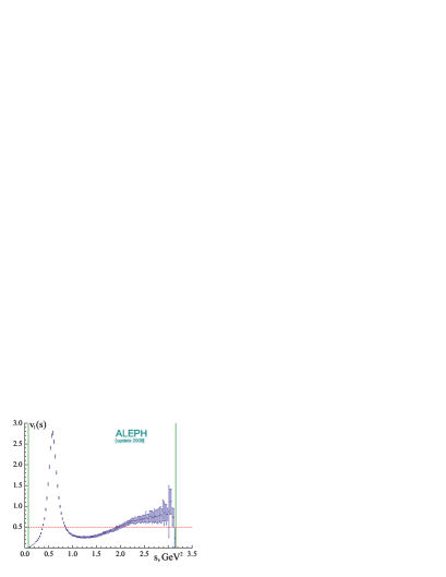
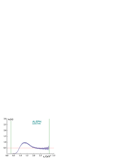
Figure 1: The inclusive vector and axial–vector spectral functions ALEPH08 . Vertical solid lines mark the boundaries of respective kinematic intervals, whereas horizontal dashed lines denote the naive massless parton model prediction.

In Eq. (3) $M_{l}$ denotes the mass of the lepton on hand, whereas $m_{\mbox{\tiny V/A}}$ stands for the total mass of the lightest allowed hadronic decay mode of this lepton in the corresponding channel. The nonvanishing value of $m_{\mbox{\tiny V/A}}$ explicitly embodies the physical fact that $\tau$ lepton is the only lepton which is heavy enough ($M_{\tau}\simeq 1.777\,$GeV PDG2012 ) to decay into hadrons. Indeed, in the massless limit ($m_{\mbox{\tiny V/A}}=0$) the theoretical prediction for $\Delta^{\mbox{\tiny}}_{\mbox{\tiny QCD}}$ (3) is nonvanishing for either lepton ($l=e,\mu,\tau$), whereas in the realistic case ($m_{\mbox{\tiny V/A}}\neq 0$) Eq. (3) acquires non–zero value for the case of the $\tau$ lepton only.

In general, it is convenient to perform the theoretical analysis of inclusive $\tau$ lepton hadronic decay in terms of the Adler function Adler (the indices “V” and “A” will only be shown when relevant hereinafter)

$$D(Q^{2})=-\frac{d\,\Pi(-Q^{2})}{d\ln Q^{2}},\quad Q^{2}=-q^{2}=-s.$$ (5)

Within perturbation theory the ultraviolet behavior of this function can be approximated by power series in the strong running coupling $\alpha^{\mbox{\scriptsize$$}}_{\mbox{\scriptsize s}}(Q^{2})$: $D(Q^{2})\simeq D^{\mbox{\scriptsize$(\ell)$}}_{\mbox{\scriptsize pert}}(Q^{2})$ for $Q^{2}\to\infty$, where

$$D^{\mbox{\scriptsize$(\ell)$}}_{\mbox{\scriptsize pert}}(Q^{2})=1+\sum\nolimits_{j=1}^{\ell}d_{j}\Bigl{[}\alpha^{\mbox{\scriptsize$(\ell)$}}_{\mbox{\scriptsize pert}}(Q^{2})\Bigr{]}^{j}.$$ (6)

At the one–loop level (i.e., for $\ell=1$) $\alpha^{\mbox{\scriptsize$(1)$}}_{\mbox{\scriptsize pert}}(Q^{2})=4\pi/(\beta_{0}\,\ln z)$, $z=Q^{2}/\Lambda^{2}$, $\beta_{0}=11-2n_{\mbox{\scriptsize f}}/3$, $\Lambda$ denotes the QCD scale parameter, $n_{\mbox{\scriptsize f}}$ is the number of active flavors, and $d_{1}=1/\pi$, see papers AdlerPert4Lab ; AdlerPert4Lc and references therein for the details. In what follows the one–loop level with $n_{\mbox{\scriptsize f}}=3$ active flavors will be assumed.

For the beginning, let us study the massless limit, that implies that the masses of all final state particles are neglected ($m=0$). By making use of definitions (4) and (5), integrating by parts, and additionally employing Cauchy theorem, the quantity $\Delta^{\mbox{\tiny}}_{\mbox{\tiny QCD}}$ (3) can be represented as (see Refs. P91 ; DP92 ; BNP )

$$\Delta^{\mbox{\tiny}}_{\mbox{\tiny QCD}}\!=\!\frac{1}{2\pi}\!\!\int_{-\pi}^{\pi}\!\!\!D\bigl{(}M_{\tau}^{2}\,e^{i\theta}\bigr{)}\bigl{(}1\!+\!2e^{i\theta}\!-\!2e^{i3\theta}\!-\!e^{i4\theta}\bigr{)}d\theta.$$ (7)

It is necessary to outline here that Eq. (7) can be derived from Eq. (3) only for the massless limit of “genuine physical” Adler function $D^{\mbox{\scriptsize$$}}_{\mbox{\scriptsize phys}}(Q^{2})$, which possesses the correct analytic properties in the kinematic variable $Q^{2}$. However, in Eq. (7) one usually directly employs the perturbative approximation $D^{\mbox{\scriptsize$$}}_{\mbox{\scriptsize pert}}(Q^{2})$ (6), which has unphysical singularities in $Q^{2}$. At the one–loop level this prescription eventually leads to

$$\Delta^{\mbox{\scriptsize$$}}_{\mbox{\scriptsize pert}}\!=\!\Delta^{\mbox{\scriptsize$(0)$}}_{\mbox{\scriptsize pert}}\!+\!\frac{4}{\beta_{0}}\!\int_{0}^{\pi}\frac{\lambda A_{1}(\theta)+\theta A_{2}(\theta)}{\pi(\lambda^{2}+\theta^{2})}\,d\theta,$$ (8)

where $A_{1}(\theta)=1+2\cos(\theta)-2\cos(3\theta)-\cos(4\theta)$, $A_{2}(\theta)\!=\!2\sin(\theta)-2\sin(3\theta)-\sin(4\theta)$, $\lambda\!=\!\ln\bigl{(}M_{\tau}^{2}/\Lambda^{2}\bigr{)}$, and $\Delta^{\mbox{\scriptsize$(0)$}}_{\mbox{\scriptsize pert}}=1$.

          

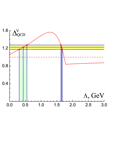
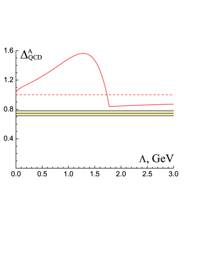
Figure 2: Comparison of the one–loop perturbative expression $\Delta^{\mbox{\tiny$$}}_{\mbox{\tiny pert}}$ (8) (solid curves) with relevant experimental data (9) (horizontal shaded bands). The solution for QCD scale parameter $\Lambda$ (if exists) is shown by vertical dashed band.

It is worth noting also that perturbative approach provides identical predictions for functions (3) in vector and axial–vector channels (i.e., $\Delta^{\mbox{\scriptsize$\mbox{\tiny V}$}}_{\mbox{\scriptsize pert}}\equiv\Delta^{\mbox{\scriptsize$\mbox{\tiny A}$}}_{\mbox{\scriptsize pert}}$). However, their experimental values ALEPH9806 ; ALEPH08 are different, namely

$$\Delta^{\mbox{\scriptsize$\mbox{\tiny V}$}}_{\mbox{\scriptsize exp}}\!\!=\!1.224\!\pm\!0.050,\quad\!\Delta^{\mbox{\scriptsize$\mbox{\tiny A}$}}_{\mbox{\scriptsize exp}}\!\!=\!0.748\!\pm\!0.034.$$ (9)

The juxtaposition of these quantities with perturbative result (8) is presented in Fig. 2. As one can infer from this figure, for vector channel there are two solutions for the QCD scale parameter, namely, $\Lambda=\bigl{(}434^{+117}_{-127}\bigr{)}\,$MeV and $\Lambda=\bigl{(}1652^{+21}_{-23}\bigr{)}\,$MeV. Commonly, the first of these solutions is retained, whereas the second one is merely disregarded. As for the axial–vector channel, the perturbative approach fails to describe the experimental data on inclusive $\tau$ lepton hadronic decay, since for any value of $\Lambda$ the function $\Delta^{\mbox{\scriptsize$$}}_{\mbox{\scriptsize pert}}$ (8) exceeds $\Delta^{\mbox{\scriptsize$\mbox{\tiny A}$}}_{\mbox{\scriptsize exp}}$ (9).

It is crucial to emphasize that the presented above massless limit completely leaves out the effects due to hadronization, which play an important role in the studies of the strong interaction processes at low energies. Specifically, the mathematical realization of the physical fact, that in a strong interaction process no hadrons can be produced at energies below the total mass $m$ of the lightest allowed hadronic final state, consists in the fact that the beginning of cut of corresponding hadronic vacuum polarization function $\Pi(q^{2})$ in complex $q^{2}$–plane is located at the threshold of hadronic production $q^{2}=m^{2}$, but not at $q^{2}=0$. Such restrictions are inherently embodied within relevant dispersion relation. In turn, the latter imposes stringent physical nonperturbative constraints on the quantities on hand, which should certainly be accounted for when one is trying to go beyond the limitations of perturbation theory.

Thus, the nonperturbative constraints, which dispersion relation Adler

$$D(Q^{2})=Q^{2}\!\int_{m^{2}}^{\infty}\!\frac{R(s)}{(s+Q^{2})^{2}}\,ds$$ (10)

imposes on the Adler function (5), have been merged with corresponding perturbative result (6) in the framework of Dispersive approach to QCD, that has eventually led to the following integral representations for functions (4) and (5) (see Refs. MAPT2 ; NPQCD07 for the details):

$$R(s)\!\!\!\! = \!\!\!\!r^{\mbox{\scriptsize$(0)$}}_{\mbox{\scriptsize}}(s)+\theta\Bigl{(}1-\frac{m^{2}}{s}\Bigr{)}\!\int_{s}^{\infty}\!\rho(\sigma)\,\frac{d\sigma}{\sigma}\,,$$ (11)

$$D(Q^{2})\!\!\!\! = \!\!\!\!d^{\mbox{\scriptsize$(0)$}}_{\mbox{\scriptsize}}(Q^{2})+\!\!\int_{m^{2}}^{\infty}\!\!\!P(Q^{2},m^{2},\sigma)\,\rho(\sigma)\,\frac{d\sigma}{\sigma}.$$ (12)

In these equations $\rho(\sigma)$ denotes the spectral density, $P(Q^{2},m^{2},\sigma)=Q^{2}(\sigma-m^{2})/((Q^{2}+m^{2})(\sigma+Q^{2}))$, and $\theta(x)$ is the unit step–function ($\theta(x)=1$ if $x\geq 0$ and $\theta(x)=0$ otherwise). It is worth noting also that in the massless limit ($m=0$) expressions (11) and (12) become identical to those of the so–called Analytic Perturbation Theory APTSS ; APTMS (see also Refs. Cvetic ; APT1 ; APT2 ). But, as it was mentioned above, it is essential to keep the hadronic mass $m$ nonvanishing within the approach on hand.

          

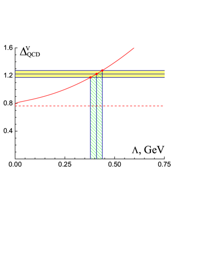
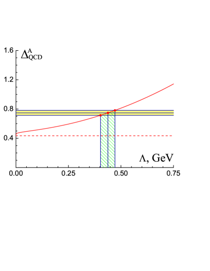
Figure 3: Comparison of expression $\Delta^{\mbox{\tiny$\!\mbox{V/A}$}}_{\mbox{\tiny QCD}}$ (16) (solid curves) with relevant experimental data (9) (horizontal shaded bands). The solutions for QCD scale parameter $\Lambda$ are shown by vertical dashed bands.

Let us proceed now to the description of inclusive $\tau$ lepton hadronic decay within Dispersive approach MAPT2 ; NPQCD07 (see also papers PRD64 ; PRD71 ; PRD77 and references therein). In this analysis the effects due to hadronization will be retained (in other words, the expressions (11) and (12) will be used instead of their perturbative approximations and the hadronic mass $m$ will be kept nonvanishing). The so–called “smooth kinematic threshold” for the leading–order term of function $R(s)$ (see, e.g., Refs. Feynman ; QCDAB ) will also be employed:

$$r^{\mbox{\scriptsize$(0)$}}_{\mbox{\scriptsize\mbox{\tiny V/A}}}(s)\!\!\!\!\! = \!\!\!\!\!(1-m_{\mbox{\tiny V/A}}^{2}/s)^{3/2},$$ (13)

$$d^{\mbox{\scriptsize$(0)$}}_{\mbox{\scriptsize\mbox{\tiny V/A}}}(Q^{2})\!\!\!\!\! = \!\!\!\!\!1+\frac{3}{\xi}\biggl{[}\!1+\frac{u(\xi)}{2}\ln\Bigl{[}\!1\!+\!2\xi\bigl{(}1\!-\!u(\xi)\bigr{)}\Bigr{]}\biggr{]},$$ (14)

where $u(\xi)=\sqrt{1+\xi^{-1}}$ and $\xi=Q^{2}/m_{\mbox{\tiny V/A}}^{2}$. Besides, the following model for the one–loop spectral density will be adopted:

$$\rho(\sigma)=\frac{4}{\beta_{0}}\frac{1}{\ln^{2}(\sigma/\Lambda^{2})+\pi^{2}}+\frac{\Lambda^{2}}{\sigma}\,,$$ (15)

see papers Tau11 ; PRD62 ; Review and references therein. The first term in the right–hand side of Eq. (15) is the one–loop perturbative contribution, whereas the second term represents intrinsically nonperturbative part of the spectral density.

Eventually, all this has led to the following expression for the quantity $\Delta^{\mbox{\tiny V/A}}_{\mbox{\tiny QCD}}$ (3) within Dispersive approach (see Refs. Tau11 ; Prep for the details):

$$\Delta^{\mbox{\tiny V/A}}_{\mbox{\tiny QCD}}\!\!\!\!\! = \!\!\!\!\!\sqrt{1-\zeta_{\mbox{\tiny V/A}}}\,\biggl{(}1+6\zeta_{\mbox{\tiny V/A}}-\frac{5}{8}\zeta_{\mbox{\tiny V/A}}^{2}+\frac{3}{16}\zeta_{\mbox{\tiny V/A}}^{3}\biggr{)}$$ (16)

$$-3\zeta_{\mbox{\tiny V/A}}\biggl{(}1+\frac{1}{8}\zeta_{\mbox{\tiny V/A}}^{2}-\frac{1}{32}\zeta_{\mbox{\tiny V/A}}^{3}\biggr{)}$$

$$~{}\,\times\ln\biggl{[}\frac{2}{\zeta_{\mbox{\tiny V/A}}}\Bigl{(}1+\sqrt{1-\zeta_{\mbox{\tiny V/A}}}\Bigr{)}-1\biggr{]}$$

$$+\int_{m_{\mbox{\tiny V/A}}^{2}}^{\infty}\!H\biggl{(}\frac{\sigma}{M_{\tau}^{2}}\biggr{)}\,\rho(\sigma)\,\frac{d\sigma}{\sigma}\,,$$

where $H(x)=g(x)\,\theta(1-x)+g(1)\,\theta(x-1)-g(\zeta_{\mbox{\tiny V/A}})$, $g(x)=x(2-2x^{2}+x^{3})$, $m_{\mbox{\tiny V}}^{2}\simeq 0.075\,\mbox{GeV}^{2}$, $m_{\mbox{\tiny A}}^{2}\simeq 0.300\,\mbox{GeV}^{2}$, and $\zeta_{\mbox{\tiny V/A}}=m_{\mbox{\tiny V/A}}^{2}/M_{\tau}^{2}$.

The comparison of obtained result (16) with experimental data (9) yields nearly identical solutions for the QCD scale parameter $\Lambda$ in both channels, see Fig. 3. Namely, $\Lambda=(408\pm 30)\,$MeV for vector channel and $\Lambda=(437\pm 34)\,$MeV for axial–vector one. Additionally, both these solutions agree with aforementioned perturbative solution for vector channel.

The author is grateful to A. Bakulev, D. Boito, M. Davier, and S. Menke for the stimulating discussions and useful comments. Partial financial support of grant JINR–12–301–01 is acknowledged.

References

• (1) M. Davier, S. Descotes–Genon, A. Hocker, B. Malaescu, and Z. Zhang, Eur. Phys. J. C 56 (2008) 305.
• (2) J. Beringer et al. [Particle Data Group Collaboration], Phys. Rev. D 86 (2012) 010001.
• (3) E. Braaten, S. Narison, and A. Pich, Nucl. Phys. B 373 (1992) 581.
• (4) W.J. Marciano and A. Sirlin, Phys. Rev. Lett. 61 (1988) 1815; E. Braaten and C.S. Li, Phys. Rev. D 42 (1990) 3888.
• (5) S.L. Adler, Phys. Rev. D 10 (1974) 3714.
• (6) P.A. Baikov, K.G. Chetyrkin, and J.H. Kuhn, Phys. Rev. Lett. 101 (2008) 012002; 104 (2010) 132004.
• (7) P.A. Baikov, K.G. Chetyrkin, J.H. Kuhn, and J. Rittinger, Phys. Lett. B 714 (2012) 62.
• (8) A.A. Pivovarov, Z. Phys. C 53 (1992) 461.
• (9) F. Le Diberder and A. Pich, Phys. Lett. B 286 (1992) 147; 289 (1992) 165.
• (10) R. Barate et al. [ALEPH Collaboration], Eur. Phys. J. C 4 (1998) 409; M. Davier, A. Hocker, and Z. Zhang, Rev. Mod. Phys. 78 (2006) 1043.
• (11) A.V. Nesterenko and J. Papavassiliou, J. Phys. G 32 (2006) 1025.
• (12) A.V. Nesterenko, SLAC eConf C0706044 (2008) 25; arXiv:0710.5878 [hep-ph]; Nucl. Phys. B (Proc. Suppl.) 186 (2009) 207.
• (13) D.V. Shirkov and I.L. Solovtsov, Phys. Rev. Lett. 79 (1997) 1209; Theor. Math. Phys. 150 (2007) 132.
• (14) K.A. Milton and I.L. Solovtsov, Phys. Rev. D 55 (1997) 5295; 59 (1999) 107701.
• (15) G. Cvetic and C. Valenzuela, Braz. J. Phys. 38 (2008) 371.
• (16) K.A. Milton, I.L. Solovtsov, and O.P. Solovtsova, Mod. Phys. Lett. A 21 (2006) 1355; G. Cvetic, C. Valenzuela, and I. Schmidt, Nucl. Phys. B (Proc. Suppl.) 164 (2007) 308.
• (17) A.P. Bakulev, Phys. Part. Nucl. 40 (2009) 715; G. Cvetic and A.V. Kotikov, J. Phys. G 39 (2012) 065005.
• (18) A.V. Nesterenko, Phys. Rev. D 64 (2001) 116009.
• (19) A.V. Nesterenko and J. Papavassiliou, Phys. Rev. D 71 (2005) 016009.
• (20) M. Baldicchi, A.V. Nesterenko, G.M. Prosperi, and C. Simolo, Phys. Rev. D 77 (2008) 034013.
• (21) R.P. Feynman, Photon–hadron interactions, Reading, MA: Benjamin (1972) 282p.
• (22) A.I. Akhiezer and V.B. Berestetsky, Quantum electrodynamics, Interscience, NY (1965) 868p.
• (23) A.V. Nesterenko, SLAC eConf C1106064 (2011) 23; arXiv:1106.4006 [hep-ph]; arXiv:1110.3415 [hep-ph].
• (24) A.V. Nesterenko, Phys. Rev. D 62 (2000) 094028.
• (25) A.V. Nesterenko, Int. J. Mod. Phys. A 18 (2003) 5475; Nucl. Phys. B (Proc. Suppl.) 133 (2004) 59.
• (26) A.V. Nesterenko, in preparation.