Non-perturbative theoretical description of two atoms in an optical lattice with time-dependent perturbations

Abstract

A theoretical approach for a non-perturbative dynamical description of two interacting atoms in an optical lattice potential is introduced. The approach builds upon the stationary eigenstates found by a procedure described in Grishkevich et al. [Phys. Rev. A 84, 062710 (2011)]. It allows presently to treat any time-dependent external perturbation of the lattice potential up to quadratic order. Example calculations of the experimentally relevant cases of an acceleration of the lattice and the turning-on of an additional harmonic confinement are presented.

I Introduction

Triggered by the creation of the first Bose-Einstein condensates Anderson et al. (1995); Davis et al. (1995), the field of ultracold atoms has experienced many major advancements. Nowadays it is not only possible to steer and observe many-body effects like the Mott-insulator superfluid phase transition Greiner et al. (2002); Bloch et al. (2008); Bakr et al. (2010) but also to manipulate single atoms in an optical lattice (OL) or a dipole trap Weitenberg et al. (2011); Serwane et al. (2011).

A key technology is the dynamical variation of the trapping potential that allows, e.g., for a cooling of the system by transferring hot atoms to non-trapped continuum states Bakr et al. (2011). In a recent work by some of us it has been proposed how to perform quantum computations in an OL just by manipulating the depth of single lattice sites and by shaking the optical lattice to drive transitions between different Bloch bands Schneider and Saenz (2012). For a full understanding of the underlying dynamical processes of any multi-band system Anderlini et al. (2007); Trotzky et al. (2008); Wirth et al. (2010); Bakr et al. (2011) the application of the usually employed single-band Hubbard model is insufficient. Here, a numerical approach is presented, that solves the full time-dependent Schrödinger equation of two interacting atoms in a single-well or multiple-well lattice, which can be perturbed by any additional time-dependent potential up to quadratic order. While the types of perturbations can be easily extended, the currently implemented types already allow for studying many experimentally relevant situations. For example, an acceleration of an OL or a periodic driving as realized in Ivanov et al. (2008); Sias et al. (2008) results in a linear perturbation of the lattice. The manipulation of the barrier hight between two lattice sites Anderlini et al. (2007) or a variation of the global confinement, e.g. by a MOT Schneider et al. (2008), can be simulated by adding a harmonic perturbation.

The general problem of a precise description of interacting atoms in trapping potentials is the existence of two very distinct length scales: that of the short-range Born-Oppenheimer interaction (some 100 a.u.) and that of the trapping potential (some $10\,000$ a.u.). The employed basis functions have to cover the highly oscillating behavior in the interaction range and the slow variation due to the trap. The use of an uncorrelated basis such as a regular grid or products of single-particle solutions is therefore impractical. A method to avoid the length scale problem is to replace the interaction potential by a delta-like pseudo potential that supports only a single bound state and can be adjusted to have the same $s$-wave scattering length as the full interaction potential Busch et al. (1998). In this case the problem can be tackled, e.g., by choosing a basis of multi-band Wannier functions of the optical lattice Schneider and Saenz (2012). However, effects of higher partial waves or of an energy dependence of the scattering length, that can easily become important if multiple Bloch bands are occupied Schneider et al. (2011), are ignored by this approach. Here, the problem is approached by using the stationary solutions of the lattice potential obtained by a procedure presented in Grishkevich et al. (2011). For this, the Hamiltonian is first separated into relative (rel.) motion and center-of-mass (c.m.) motion. The different length scales are covered by expanding the rel. and c.m. wave functions in spherical harmonics and a flexible basis of $B$ splines for the radial part Grishkevich et al. (2011). In a configuration-interaction procedure the eigenfunctions of the rel. and c.m. part of the full lattice Hamiltonian are used to determine the full eigenfunctions. These eigenfunctions are subsequently used as a basis for the propagation of the time-dependent wavefunction.

The paper is organized as follows. In Sec. II the stationary Hamiltonian of the system is presented. In order to understand the numerical approach, the basis functions obtained by the procedure in Grishkevich et al. (2011) are shortly introduced while the interested reader should consult Grishkevich et al. (2011) for a more detailed description. In Sec. III the time-propagation method is described. Afterwards in Sec. IV the results of the time propagation are validated by a comparison to problems that possess an analytical solution. Finally, in Sec. V the numerical method is used to analyse a system of ⁶Li-⁷Li in a three-well OL. The experimentally relevant cases of an acceleration of the lattice, i. e., a linear perturbation, and of an additional harmonic confinement are considered.

II Stationary Hamiltonian and its eigensolutions

The full Hamiltonian

$$\hat{H}(t)=\hat{H}_{0}+\hat{W}(t)\\$$ (1)

consists of a time-dependent part $\hat{W}(t)$ (specified below) and a stationary part

$$\hat{H}_{0}=\frac{\hat{p}_{1}^{2}}{2m_{1}}+\frac{\hat{p}_{2}^{2}}{2m_{2}}+\hat{V}_{\rm lat}^{(1)}(\vec{r}_{1}\,)+\hat{V}_{\rm lat}^{(2)}(\vec{r}_{2}\,)+\hat{V}_{\rm int}(\vec{r}_{1}-\vec{r}_{2}\,)$$ (2)

for two particles $i=1,2$ with mass $m_{i}$ interacting via the potential $\hat{V}_{\rm int}$. In the case of ultracold atoms the isotropic interaction potential $\hat{V}_{\rm int}(\vec{r}_{1}-\vec{r}_{2}\,)=\hat{V}_{\rm int}(|\vec{r}_{1}-\vec{r}_{2}\,|)$ is described by an often only numerically given Born-Oppenheimer potential. The trapping potential

$$\hat{V}_{\rm lat}^{(i)}=\sum_{u=x,y,z}V_{u}^{(i)}\sin^{2}(k_{u}u_{i})$$ (3)

is that of an OL formed by three counter-propagating laser beams with wave vector $k_{u}$ in $u$ direction ($u=x,y,z$). The lattice depth $V_{u}^{(i)}$ is proportional to the laser intensity in direction $u$ and the polarizability of particle $i$.

The infinite lattice potential $V_{\rm lat}$ is reduced to a potential $\tilde{V}_{\rm lat}$ with finite extension by expanding $V_{\rm lat}$ to some arbitrary order into a Taylor series in all three directions [see Fig. 1 for the example of a 22nd order expansion of $V_{x}\sin^{2}(k_{x}x)$]. For practical purposes only expansions of order $2(2n+1)$ are important, which lead to lattice potentials $\tilde{V}_{\rm lat}$ with $\tilde{V}_{\rm lat}(\vec{r}\,)\rightarrow\infty$ for $|\vec{r}\,|\rightarrow\infty$. For other expansions the potential is unbound from below leading to the appearance of non-physical states.

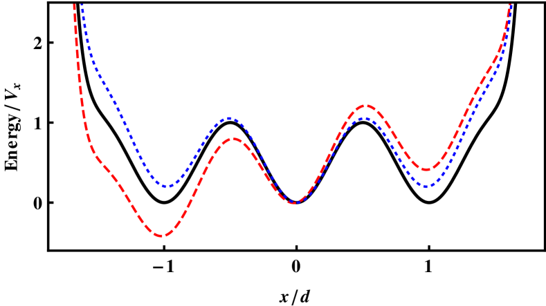
Figure 1: (color online) The 22nd-order expansion $\tilde{V}_{\rm lat}(x,y=0,z=0)$ of the lattice potential $V_{\rm lat}(x,y=0,z=0)$ in $x$-direction (solid line). Lengths are given in units of the lattice spacing $d=\pi/k_{x}$. A linear perturbation as it appears, e.g., for an acceleration of the lattice in $x$ direction leads to an inclination of the lattice sketched by the red dashed line, while an additional harmonic confinement raises the left and right lattice site (blue dotted line).

The trapping potential $\hat{V}_{\rm lat}$ of an OL (and also $\tilde{V}_{\rm lat}$) has orthorhombic symmetry, which is characterized by the point group $D_{2h}$. By adapting the basis functions to this symmetry, the eigenfunctions and the time-dependent wave function can be determined more efficiently. The symmetry of the problem is discussed in depth in Grishkevich et al. (2011). Here, only the essential points are repeated.

The symmetry operations of $D_{2h}$ are

$$\mathcal{S}=\left\{E,\;C_{2}(x),\;C_{2}(y),\;C_{2}(z),\;\sigma(xy),\;\sigma(xz),\;\sigma(yz),\;i\right\}\,,$$ (4)

where $E$ is the identity, $C_{n}(u)$ is the rotation about $\frac{2\pi}{n}$ around the $u$ axis ($u=x,y,z$), $\sigma(u_{1}u_{2})$ the reflection on the ($u_{1}$, $u_{2}$) plane and $i$ the inversion (i. e. point reflection at the origin).

Since the interaction potential $\hat{V}_{\rm int}$ is invariant under any operation in $\mathcal{S}$ also the full unperturbed Hamiltonian $\hat{H}_{0}$ belongs to the $D_{2h}$ point group if the symmetry operations are performed on both coordinates $\vec{r}_{1}$ and $\vec{r}_{2}$ simultaneously.

The group $D_{2h}$ possesses eight irreducible representations $\Gamma_{\sigma}$ with

$$\sigma\in\left\{A_{g},B_{1g},B_{2g},B_{3g},A_{u},B_{1u},B_{2u},B_{3u}\right\}\,.$$ (5)

The characters of these irreducible representations are listed in Table 1.

$D_{2h}$	$E$	$C_{2}(z)$	$C_{2}(y)$	$C_{2}(x)$	$i$	$\sigma(xy)$	$\sigma(xz)$	$\sigma(yz)$
$A_{g}$	1	1	1	1	1	1	1	1
$B_{1g}$	1	1	-1	-1	1	1	-1	-1
$B_{2g}$	1	-1	1	-1	1	-1	1	-1
$B_{3g}$	1	-1	-1	1	1	-1	-1	1
$A_{u}$	1	1	1	1	-1	-1	-1	-1
$B_{1u}$	1	1	-1	-1	-1	-1	1	1
$B_{2u}$	1	-1	1	-1	-1	1	-1	1
$B_{3u}$	1	-1	-1	1	-1	1	1	-1

Table 1: Character table of the $D_{2h}$ point group.

In order to find the eigensolutions of $\hat{H}_{0}$ the system is split into rel. and c.m. coordinates,

$$\vec{\rho}=\vec{r_{1}}-\vec{r_{2}}\,,\quad\vec{R}=\frac{m_{1}\vec{r_{1}}+m_{2}\vec{r_{2}}}{m_{1}+m_{2}}.$$ (6)

With this separation, the Hamiltonian is written as

$$\hat{H}_{0}(\vec{R},\vec{\rho}\,)=\hat{H}_{\rm c.m.\ }(\vec{R})+\hat{H}_{\rm rel.\ }(\vec{\rho}\,)+\hat{H}_{\rm coupl\ }(\vec{R},\vec{\rho}\,)\,,$$ (7)

where $\hat{H}_{\rm c.m.}$, $\hat{H}_{\rm rel.}$, and $\hat{H}_{\rm coupl\ }(\vec{R},\vec{\rho}\,)$ still have $D_{2h}$-symmetry Grishkevich et al. (2011).

The eigenfunctions of rel. and c.m. are described in spherical coordinates and expanded in a basis of $B$ splines $B_{\alpha}$ and spherical harmonics $Y_{l}^{m}$. Since the symmetry operations of $D_{2h}$ commute with the Hamiltonian, the eigenfunctions can be chosen such that their symmetry properties correspond to some irreducible representation $\Gamma_{\sigma}$ of $D_{2h}$. In the following the rel. (c.m.) eigenfunctions are denoted as $\phi_{j}^{(\sigma)}(\vec{\rho}\,)$ [$\Psi_{j}^{(\sigma)}(\vec{R})$] with $j=1,2,3,\dots$

In a configuration-interaction procedure products of eigensolutions of $\hat{H}_{\rm c.m.}$ and $\hat{H}_{\rm rel.}$, i.e. configurations, are used to diagonalize the full Hamiltonian $\hat{H}_{0}$. Because all irreducible representations of $D_{2h}$ are one dimensional, the direct product of two irreducible representations $\Gamma_{\kappa}\otimes\Gamma_{\lambda}$ is again an irreducible representation $\Gamma_{\sigma}$ that can be determined from the product table 2. Hence, each configuration $\Psi_{i}^{(\kappa)}(\vec{R})\phi_{j}^{(\lambda)}(\vec{\rho}\,)$ has the symmetry properties of the related irreducible representation $\Gamma_{\sigma}=\Gamma_{\kappa}\otimes\Gamma_{\lambda}$. The full solutions of a given symmetry $\sigma$ has the form of a superposition

$$\Phi_{\sigma}(\vec{R},\vec{\rho}\,)=\sum_{\left\{\kappa,\lambda\right\}\in\sigma}\sum_{ij}\mathcal{C}_{ij}^{(\kappa,\lambda)}\Psi_{i}^{(\kappa)}(\vec{R})\phi_{j}^{(\lambda)}(\vec{\rho}\,)\,,$$ (8)

where $\left\{\kappa,\lambda\right\}\in\sigma$ should indicate that the summation is performed over irreducible representations that fulfill $\Gamma_{\kappa}\otimes\Gamma_{\lambda}=\Gamma_{\sigma}$.

When considering identical bosonic (fermionic) particles the rel. wavefunction has to be symmetric (antisymmetric) under inversion, i. e. only basis functions of rel. motion with $\lambda\in\{A_{g},B_{1g},B_{2g},B_{3g}\}$ ($\lambda\in\{A_{u},B_{1u},B_{2u},B_{3u}\}$) are used to form configurations.

The wavefunctions, i. e. the coefficients $C_{ij}^{(\kappa,\lambda)}$ in Eq. (8), are finally determined by solving the eigenvalue problem

$$\hat{H}_{0}\left|\Phi_{i}^{(\sigma)}\right>=E_{i}^{(\sigma)}\left|\Phi_{i}^{(\sigma)}\right>$$ (9)

of $\hat{H}_{0}$ in the configuration basis.

$\otimes$	$A_{g}$	$B_{1g}$	$B_{2g}$	$B_{3g}$	$A_{u}$	$B_{1u}$	$B_{2u}$	$B_{3u}$
$A_{g}$	$A_{g}$	$B_{1g}$	$B_{2g}$	$B_{3g}$	$A_{u}$	$B_{1u}$	$B_{2u}$	$B_{3u}$
$B_{1g}$	$B_{1g}$	$A_{g}$	$B_{3g}$	$B_{2g}$	$B_{1u}$	$A_{u}$	$B_{3u}$	$B_{2u}$
$B_{2g}$	$B_{2g}$	$B_{3g}$	$A_{g}$	$B_{1g}$	$B_{2u}$	$B_{3u}$	$A_{u}$	$B_{1u}$
$B_{3g}$	$B_{3g}$	$B_{2g}$	$B_{1g}$	$A_{g}$	$B_{3u}$	$B_{2u}$	$B_{1u}$	$A_{u}$
$A_{u}$	$A_{u}$	$B_{1u}$	$B_{2u}$	$B_{3u}$	$A_{g}$	$B_{1g}$	$B_{2g}$	$B_{3g}$
$B_{1u}$	$B_{1u}$	$A_{u}$	$B_{3u}$	$B_{2u}$	$B_{1g}$	$A_{g}$	$B_{3g}$	$B_{2g}$
$B_{2u}$	$B_{2u}$	$B_{3u}$	$A_{u}$	$B_{1u}$	$B_{2g}$	$B_{3g}$	$A_{g}$	$B_{1g}$
$B_{3u}$	$B_{3u}$	$B_{2u}$	$B_{1u}$	$A_{u}$	$B_{3g}$	$B_{2g}$	$B_{1g}$	$A_{g}$

Table 2: Product table of irreducible representations of the $D_{2h}$ point group.

III Time-dependent evolution

The Schrödinger equation of the time-dependent evolution

$$\begin{split}\left(\hat{H}_{0}+\hat{W}(t)\right)\left|\Psi(t)\right>&=i\hbar\frac{\partial}{\partial t}\left|\Psi(t)\right>\\ \text{with}\quad\left|\Psi(t=0)\right>&=\left|\Psi_{0}\right>\end{split}$$ (10)

is solved in the basis $\{\Phi_{i}^{(\sigma)}\}$ of eigenfunctions of $\hat{H}_{0}$ of Eq. (9),

$$\left|\Psi(t)\right>=\sum_{\sigma i}\mathcal{B}_{\sigma i}(t)\left|\Phi_{i}^{(\sigma)}\right>\,.$$ (11)

Plugging Eq. (11) into Eq. (10) and multiplying from the left by $\left<\Phi_{j}^{(\kappa)}\right|$ leads to the equation

$$i\hbar\frac{\partial\mathcal{B}_{\kappa j}(t)}{\partial t}=E_{j}^{(\kappa)}\mathcal{B}_{\kappa j}(t)+\sum_{\sigma i}\mathcal{B}_{\sigma i}(t)\left<\Phi_{j}^{(\kappa)}\right|\hat{W}(t)\left|\Phi_{i}^{(\sigma)}\right>$$ (12)

for the evolution of the time-dependent coefficients $\mathcal{B}_{\kappa j}(t)$, which is governed by the matrix elements $\mathcal{P}_{ij}^{(\kappa,\sigma)}=\left<\Phi_{j}^{(\kappa)}\right|\hat{W}(t)\left|\Phi_{i}^{(\sigma)}\right>$ of the perturbation. Considering two eigenstates

$$\begin{split}\left|\Phi_{m}^{(\tau)}\right>=&\sum_{\left\{\kappa,\lambda\right\}\in\tau}\sum_{ij}\mathcal{C}_{ij}^{(\kappa,\lambda)}\left|\Psi_{i}^{(\kappa)}\right>\left|\phi_{j}^{(\lambda)}\right>\\ \left|\Phi_{n}^{(\sigma)}\right>=&\sum_{\left\{\mu,\nu\right\}\in\sigma}\sum_{kl}\mathcal{C^{\prime}}_{kl}^{(\mu,\nu)}\left|\Psi_{k}^{(\mu)}\right>\left|\phi_{l}^{(\nu)}\right>\\ \end{split}$$ (13)

as specified in Eq. (8), the matrix elements of a perturbation are

$$\begin{split}\mathcal{P}_{mn}^{(\tau,\sigma)}=&\left<\Phi_{m}^{(\tau)}\right|\hat{W}(t)\left|\Phi_{n}^{(\sigma)}\right>\\ =&\sum_{\left\{\kappa,\lambda\right\}\in\tau}\sum_{ij}\sum_{\left\{\mu,\nu\right\}\in\sigma}\sum_{kl}\left(\mathcal{C}_{ij}^{(\kappa,\lambda)}\right)^{*}\mathcal{C^{\prime}}_{kl}^{(\mu,\nu)}\\ &\times\left<\phi_{j}^{(\lambda)}\right|\left<\Psi_{i}^{(\kappa)}\right|\hat{W}(t)\left|\Psi_{k}^{(\mu)}\right>\left|\phi_{l}^{(\nu)}\right>\,.\end{split}$$ (14)

In general, the perturbation $\hat{W}(t)$ can be expanded in a time-dependent Taylor series of its spacial coordinates

$$\hat{W}(t)=\sum_{nm}\sum_{u=x,y,z}\sum_{u^{\prime}=x,y,z}f_{nm}^{(u,u^{\prime})}(t)\,\hat{R}_{u}^{n}\,\hat{\rho}_{u^{\prime}}^{m}\,,$$

where $\rho_{u}$ ($R_{u}$) is the component of the rel. (c.m.) motion in $u$ direction ($u=x,y,z$).

At the present stage perturbations in $x$ direction of the general form

$$\begin{split}\hat{W}(t)=&f_{01}(t)\,\hat{\rho}_{x}+f_{10}(t)\,\hat{R}_{x}+f_{11}(t)\,\hat{\rho}_{x}\hat{R}_{x}\\ &+f_{02}(t)\,\hat{\rho}_{x}^{2}+f_{20}(t)\,\hat{R}_{x}^{2}\end{split}$$ (15)

are implemented. In principle, the method can be easily extended to allow for perturbations in other directions and of higher orders.

In order to illustrate how the perturbation matrix is computed, the case of a linear perturbation $\hat{W}=f_{10}(t)\hat{R}_{x}$ is discussed in more detail. This perturbation does not couple the orthonormal rel. basis functions $\left|\phi_{j}^{(\lambda)}\right>$. Thus, the summations in Eq. (14) reduce to

$$\begin{split}\mathcal{P}_{mn}^{(\tau,\sigma)}=&f_{10}(t)\sum_{\left\{\kappa,\lambda\right\}\in\tau}\sum_{ij}\sum_{\left\{\mu,\lambda\right\}\in\sigma}\sum_{k}\left(\mathcal{C}_{ij}^{(\kappa,\lambda)}\right)^{*}\mathcal{C^{\prime}}_{kj}^{(\mu,\lambda)}\\ &\left<\Psi_{i}^{(\kappa)}\right|\hat{R}_{x}\left|\Psi_{k}^{(\mu)}\right>\,.\end{split}$$ (16)

In the following the term $\left<\Psi_{i}^{(\kappa)}\right|\hat{R}_{x}\left|\Psi_{k}^{(\mu)}\right>$ is considered for the exemplary case of $\kappa=A_{g}$. In this case the wave function $\Psi_{i}^{(\kappa)}(\vec{R}\,)$ is totally symmetric (see Table 1). Hence, $\Psi_{k}^{(\mu)}(\vec{R}\,)$ needs to be anti-symmetric in $x$ direction and symmetric otherwise, which is fulfilled solely for $\mu=B_{3u}$. In all other cases the integral vanishes. The according c.m. basis functions are represented as

$$\begin{split}\Psi_{i}^{(A_{g})}(R,\Theta,\Phi)&=\sum_{\alpha=1}^{N_{\alpha}}\sum_{l=0,\{2\}}^{N_{l}}\sum_{m=0,\{2\}}^{l}c_{i,\alpha lm}^{(A_{g})}\frac{B_{\alpha}(R)}{R}\mathscr{Y}_{lm}^{+}\\ \Psi_{k}^{(B_{3u})}(R,\Theta,\Phi)&=\sum_{\alpha=1}^{N_{\alpha}}\sum_{l=1,\{2\}}^{N_{l}}\sum_{m=1,\{2\}}^{l}c_{k,\alpha lm}^{(B_{3u})}\frac{B_{\alpha}(R)}{R}\mathscr{Y}_{lm}^{-}\,,\end{split}$$ (17)

where $B_{\alpha}$ are $B$ splines, $\mathscr{Y}_{lm}^{\pm}=Y_{l}^{m}(\Theta,\Phi)\pm Y_{l}^{-m}(\Theta,\Phi)$ are a sum of spherical harmonics for $m\neq 0$, and $\mathscr{Y}_{l0}^{\pm}=Y_{l}^{0}(\Theta,\Phi)$ (see Grishkevich et al. (2011) for details). The numbers in curly brackets below the sums indicate the summation step. $N_{\alpha}$ and $N_{l}$ are variable values of the number of $B$ splines and the maximal angular momentum, respectively. With $R_{x}=R\sin\Theta\cos\Phi$ one finds

$$\begin{split}\left<\Psi_{i}^{(\kappa)}\right|&\hat{R}_{x}\left|\Psi_{k}^{(\mu)}\right>\\ =&\sum_{l=0,\{2\}}\sum_{m=0,\{2\}}^{l}\sum_{l^{\prime}=1,\{2\}}\sum_{m^{\prime}=1,\{2\}}^{l^{\prime}}\sum_{\alpha\alpha^{\prime}}\left(c_{i,\alpha lm}^{(A_{g})}\right)^{*}c_{k,\alpha lm}^{(B_{3u})}\\ &\times\int\mathrm{d}R\;B_{\alpha}(R)RB_{\alpha^{\prime}}(R)\\ &\times\int_{0}^{\pi}\sin\Theta\,\mathrm{d}\Theta\;\int_{0}^{2\pi}\mathrm{d}\Phi\;\left(\mathscr{Y}_{lm}^{+}\right)^{*}\sin\Theta\cos\Phi\mathscr{Y}_{lm}^{-}\,.\end{split}$$ (18)

Using the identities $\left(Y_{l}^{m}\right)^{*}=(-1)^{m}Y_{l}^{-m}$, $\sin\Theta\cos\Phi=\sqrt{\frac{2\pi}{3}}\left[Y_{1}^{-1}(\Theta,\Phi)-Y_{1}^{1}(\Theta,\Phi)\right]$, and

$$\begin{split}\int_{0}^{\pi}\sin\Theta\,\mathrm{d}\Theta\;\int_{0}^{2\pi}\mathrm{d}\Phi\;Y_{l_{1}}^{m_{1}}(\Theta,\Phi)Y_{l_{2}}^{m_{2}}(\Theta,\Phi)Y_{l_{3}}^{m_{3}}(\Theta,\Phi)=\\ \sqrt{\frac{(2l_{1}+1)(2l_{3}+1)(2l_{3}+1)}{4\pi}}\begin{pmatrix}l_{1}&l_{2}&l_{3}\\ 0&0&0\end{pmatrix}\begin{pmatrix}l_{1}&l_{2}&l_{3}\\ m_{1}&m_{2}&m_{3}\end{pmatrix}\,,\end{split}$$ (19)

the integral over the angles in Eq. (18) can be efficiently computed in terms of Wigner 3j-symbols $\begin{pmatrix}l_{1}&l_{2}&l_{3}\\ m_{1}&m_{2}&m_{3}\end{pmatrix}$. The other types of perturbations in Eq. (15) are treated in an analogous way.

Since the system is six dimensional the analysis in terms of the full time-dependent wavefunction is nontrivial. However, equipped with the matrix elements of all perturbations, $\left<\Phi_{i}^{(\kappa)}\right|\hat{R}_{x}\left|\Phi_{k}^{(\mu)}\right>$, $\left<\Phi_{i}^{(\kappa)}\right|\hat{R}_{x}^{2}\left|\Phi_{k}^{(\mu)}\right>$, $\left<\Phi_{i}^{(\kappa)}\right|\hat{\rho}_{x}\left|\Phi_{k}^{(\mu)}\right>$, $\left<\Phi_{i}^{(\kappa)}\right|\hat{\rho}_{x}^{2}\left|\Phi_{k}^{(\mu)}\right>$, and $\left<\Phi_{i}^{(\kappa)}\right|\hat{R}_{x}\hat{\rho}_{x}\left|\Phi_{k}^{(\mu)}\right>$ one can easily determine the expectation values of some of the most important observables. For example, the squared mean particle distance in $x$ direction is given as

$$\begin{split}\left<\rho_{x}^{2}\right>=&\left<\Psi(t)\vphantom{\hat{\rho}_{x}^{2}\Psi(t)}\right|\hat{\rho}_{x}^{2}\left|\Psi(t)\vphantom{\Psi(t)\hat{\rho}_{x}^{2}}\right>\\ =&\sum_{\sigma i}\sum_{\kappa j}\left[\mathcal{B}_{\sigma i}(t)\right]^{*}\mathcal{B}_{\kappa j}(t)\left<\Phi_{i}^{(\sigma)}\right|\hat{\rho}_{x}^{2}\left|\Phi_{j}^{(\kappa)}\right>\,.\end{split}$$

Likewise, one can determine the mean particle position or the uncertainty of the position in $x$ direction.

IV Comparison with analytical results

In order to validate the numerical procedure a comparison with analytical results is necessary, which are available for the harmonic approximation of the OL potential. In the case of two identical particles of mass $m$ in a harmonic trap the system decouples into rel. and c.m. motion with Hamiltonian

$$\hat{H}_{0}=\frac{\hat{P}^{2}}{2M}+\frac{1}{2}M\omega^{2}R^{2}+\frac{\hat{p}^{2}}{2\mu}+\frac{1}{2}m\omega^{2}\rho^{2}+V_{\rm int}(\rho)\,.$$ (20)

Here, $M=2m$, $\mu=m/2$, $\hat{P}$ is the momentum of c.m. and $\hat{p}$ the momentum of rel. motion. In the following, a linear perturbation $\hat{W}(t)=f(t)\hat{R}_{x}$ and a quadratic perturbation $\hat{W}(t)=f(t)\hat{R}_{x}^{2}$, i. e. a time-dependent acceleration and a variation of the trapping frequency, are considered. Since the c.m. part of $H_{0}$ decouples into $x,y$, and $z$ direction, only the c.m. harmonic oscillator in $x$ direction with Hamiltonian

$$\hat{H}_{\rm ho}=\frac{\hat{P}_{x}^{2}}{2M}+\frac{1}{2}M\omega^{2}\hat{R}_{x}^{2}=\hbar\omega\left(A_{\rm ho}^{2}\frac{\hat{P}^{2}}{2\hbar^{2}}+\frac{1}{2}\frac{\hat{R}_{x}^{2}}{A_{\rm ho}^{2}}\right)$$ (21)

is affected by the perturbations, where $A_{\rm ho}=\sqrt{\hbar/(M\omega)}$ is the harmonic oscillator length. The comparisons are performed for expectation values of the position

$$\bar{X}(t)=\left<\hat{R}_{x}\right>=\left<\Psi(t)\vphantom{\hat{R}_{x}\Psi(t)}\right|\hat{R}_{x}\left|\Psi(t)\vphantom{\Psi(t)\hat{R}_{x}}\right>$$ (22)

and the mean deviation from $\bar{X}$

$$\sigma(t)=\sqrt{\left<\hat{R}_{x}^{2}\right>-\left<\hat{R}_{x}\right>^{2}}\,.$$ (23)

IV.1 Periodic driving

For the case of a periodically driven harmonic oscillator with driving strength $C_{\rm shake}$ and frequency $\omega_{0}$,

$$\hat{W}_{1}(t)=\hbar\omega\,C_{\rm shake}\,\cos\left(\omega_{0}t\right)\,\frac{\hat{R}_{x}}{A_{\rm ho}}\,,$$ (24)

there exists an analytic solution Bandyopadhyay and Dattagupta (2008),

$$\psi_{n}(X,t)=e^{i\varphi(x,t)}\phi_{n}(X-\xi(t))\,,$$ (25)

where $\varphi(x,t)$ is a phase, which vanishes for $t=0$, $\phi_{n}$ is the $n$th harmonic oscillator eigenstate of $\hat{H}_{\rm ho}$, and

$$\xi(t)=\frac{A_{\rm ho}C_{\rm shake}}{1-\omega_{0}^{2}/\omega^{2}}\cos(\omega_{0}t).$$ (26)

In order to conform with the initial condition

$$\psi_{n}(X,0)=\phi_{n}(X-\xi(0))$$ (27)

the trap is shifted at $t=0$ to $\xi(0)$ by instantly adding a constant linear perturbation

$$\hat{W}_{2}=-\hbar\omega\,C_{\rm shake}\,\frac{1}{1-\omega_{0}^{2}/\omega^{2}}\,\frac{\hat{R}_{x}}{A_{\rm ho}}\,.$$ (28)

From the analytic solution one obtains straightforwardly

$$\bar{X}(t)=-A_{\rm ho}C_{\rm shake}\left[1-\cos(\omega_{0}t)\right],\quad\sigma(t)=\frac{A_{\rm ho}}{\sqrt{2}}.$$ (29)

In Fig. 2 a comparison of a numerical calculation of $\bar{X}(t)$ to the result in Eq. (29) shows very good agreement with deviations on the order of $10^{-10}$. A similar accuracy is obtained for the value of $\sigma(t)$. The deviations are due to the finiteness of the basis which, in the shown calculation, only includes basis functions with an eigenenergy below the chosen cutoff of $20\hbar\omega$. The energy cutoff can be adapted to reach higher accuracies, if needed.

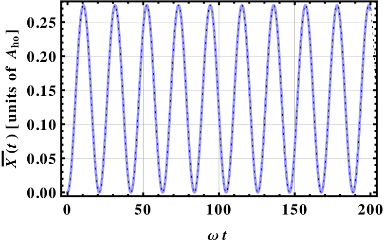
Figure 2: (color online) Comparison of analytical (blue solid) and numerical (black dashed) results for $\bar{X}(t)$ [see Eqs. (22) and (29)] for $C_{\rm shake}=0.5$. The difference of the results is below $10^{-10}$ and therefore invisible. The width of the wave function $\sigma(t)=A_{\rm ho}/\sqrt{2}$ is numerically reproduced with the same level of accuracy.

IV.2 Adiabatic deepening

The mean width of the wavefunction $\sigma$ for an harmonic oscillator with oscillator length $A_{\rm ho}$ is given as $A_{\rm ho}/\sqrt{2}$ [see Eq. (29)]. Considering a time dependent perturbation $\hat{W}(t)=C_{\rm harm}\hbar\omega\hat{R}_{x}^{2}/A_{\rm ho}^{2}\omega t$, the full potential is given as $\frac{1}{2}\hbar\omega\frac{R_{x}^{2}}{A_{\rm ho}^{2}}(1+2C_{\rm harm}\omega t)$. If the perturbation happens sufficiently slowly, the wave function will always remains in an eigenstate of a harmonic oscillator with a trap length

$$A_{\rm ho}(t)=A_{\rm ho}(t=0)/\sqrt{1+2C_{\rm harm}\omega t}\,.$$ (30)

Thus, assuming perfect adiabaticity, the width of the wave function behaves like

$$\sigma(t)=A_{\rm ho}/\sqrt{2(1+2C_{\rm harm}\omega t)}\,.$$ (31)

In Fig. 3 a comparison to the numerical calculations shows good agreement to this result with an error of about $5\times 10^{-5}$ for $C_{\rm harm}=0.002$, which is due to nonadiabatic effects. For example, reducing the speed of the perturbation by setting $C_{\rm harm}=0.001$ reduced the error to about $2\times 10^{-5}$.

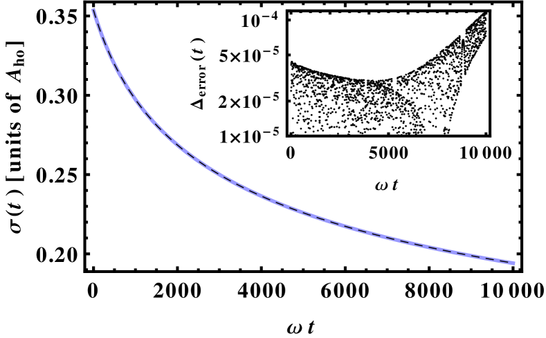
Figure 3: (color online) Comparison of analytical (blue solid) and numerical (black dashed) results for $\sigma(t)$ [see Eqs. (23) and (31)] for $C_{\rm harm}=0.002$. The error $\Delta_{\rm error}=|\sigma-\sigma_{\rm num}|$ is shown in the inset. The relatively large error in comparison to the results shown in Fig. 2 is due to nonadiabatic effects. These effects get smaller for larger $t$ since the change of $A_{\rm ho}(t)$ is reduced [see Eq. (30)]. For $\omega t>5000$, however, the incompleteness of the basis used for the numerical calculations (only states with energies below $E=20\,\hbar\omega$ are included) leads finally to an increase of $\Delta_{\rm error}$.

V Example calculations for ⁶Li-⁷Li

In the following a system of two distinguishable atoms, ⁶Li and ⁷Li is considered. The interaction potential $V_{\rm int}$ is given by the Born-Oppenheimer potential for scattering of spin-polarized lithium. The atoms are confined in a three-site lattice potential $\tilde{V}_{\rm lat}$, which is realized by a 22nd order expansion of $V_{\rm lat}$ in Eq. (3) in $x$ direction (see Fig. 1) and a harmonic approximation in $y$ and $z$ direction. The chosen wave vectors $k_{x}=k_{y}=k_{z}=2\pi/(1000\,{\rm nm})$ lead to a lattice spacing of $d=500\,{\rm nm}=9450\,$a.u. A lattice depth in $x$ direction of $V_{x}=1.36\hbar\omega_{1}$, where $\omega_{1}$ is the frequency of the harmonic approximation of the lattice for atom 1 (⁶Li), results in the relatively small hopping energies $J_{1}=2.1\times 10^{-4}\hbar\omega_{1}$ of atom 1 and $J_{2}=1.5\times 10^{-4}\hbar\omega_{1}$ of atom 2 in the corresponding Hubbard model for the infinite lattice. Hence, even for the relatively small $s$-wave scattering length of $41\,$a.u. of ⁶Li-⁷Li a correlated Mott-like state is formed, i. e., the atoms do not occupy the same lattice site in the ground state . Since no unit filling of the lattice is considered, the atoms are nevertheless mobile in $x$ direction. This enables the observation of a correlated motion of the distinguishable atoms. The lattice depths in $y$ and $z$ direction are given as $V_{y}=V_{z}\approx 8V_{x}$ such that for low-lying states motion in these directions is frozen out.

Despite the reduction to only three lattice sites, the considered system exhibits the basic mechanisms of hopping and onsite interaction of atoms in an OL. Similar systems of only a few lattice sites appear also experimentally in superlattices Anderlini et al. (2007).

V.1 Linear perturbation

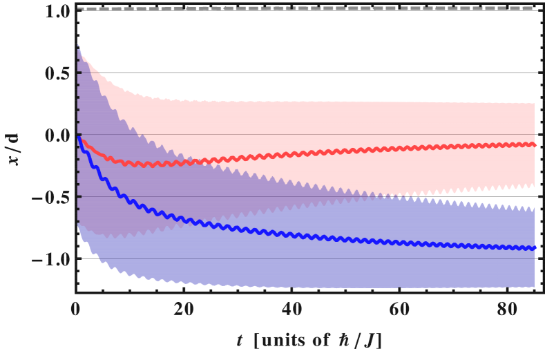
(a) x (b) x

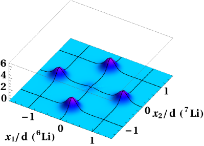
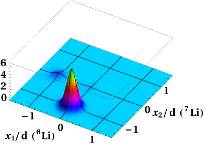
(c) x

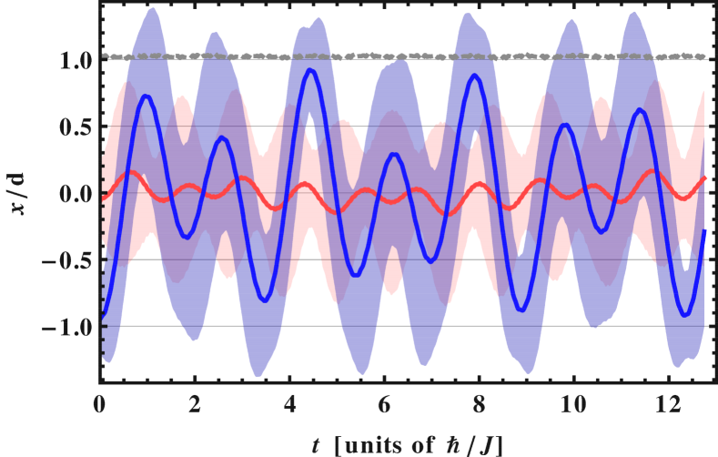
Figure 4: (color online) Mean particle position $\bar{x}_{i}=\left<x_{i}\right>$ of ⁶Li (thick lighter red line) and of ⁷Li (thick darker blue line) and mean distance $\sqrt{\left<\rho_{x}^{2}\right>}$ (grey dashed line). The corresponding lighter red, and darker blue shading illustrates the uncertainty of the position $\bar{x}_{i}\pm\sqrt{\left<(x_{i}-\bar{x}_{i})^{2}\right>}$ of ⁶Li and ⁷Li, respectively. Time is given in units of the hopping time $\hbar/J_{1}$ of ⁶Li. (a) Time dependent behavior for a linear inclination with a final perturbation $\hat{W}=66J_{1}\hat{R}_{x}/d=0.09\,\hbar\omega_{1}\hat{R}_{x}/d$. (b) Probability density $|\Psi(x_{1},x_{2})|^{2}$ for $y_{1}=y_{2}=z_{1}=z_{2}=0$ of the initial state (left) and the final state (right). Initially there is an almost equal probability of finding ⁶Li in the central well and ⁷Li in the outer wells and vice versa. After the linear inclination ⁷Li is predominantly situated in the left well and ⁶Li in the central well. The situation with exchanged ⁶Li and ⁷Li the wavefunction has a small but non-vanishing probability. (c) Free evolution of the system with the initial state being the final state of the process in (a).

First, the system is adiabatically inclined by a perturbation of the type $\hat{W}(t)=At\hat{R}_{x}$ [see Fig. 4 (a)]. Experimentally this could, e.g., be realized by slowly increasing the acceleration of the lattice in $x$ direction. The system starts in the ground state where the atoms spread symmetrically over the lattice. As a consequence, the mean atom position is exactly in the middle of the triple-well potential, i. e. at $x/d=0$. Due to their repulsion the atoms never occupy the same lattice site. In this case their mean distance $\sqrt{\left<\rho_{x}^{2}\right>}$ is approximately $d$. The corresponding probability density along the $x$ axis is shown in the left graph of Fig. 4 (b).

Upon inclining, the system stays in the state of minimal energy, i. e. the heavier ⁷Li atom slowly moves into the lower left lattice site (i. e. $\bar{x}_{2}=\left<x_{2}\right>$ approaches $-d$) while the lighter ⁶Li atom moves to the central site (i. e. $\bar{x}_{1}=\left<\hat{x}_{1}\right>$ approaches zero), where it avoids an energy gain due to the interatomic repulsion. With much smaller probability the same process with exchanged ⁶Li and ⁷Li appears [see right graph of Fig. 4 (b)]. During the process the mean distance is unchanged while the uncertainty of the position $\sqrt{\left<(x_{i}-\bar{x}_{i})^{2}\right>}$ of atom $i$ ($i=1,2$) decreases [see Fig. 4 (a) and (b)]. Stopping at a final inclination that results in an energy difference of $0.09\hbar\omega$ between neighboring wells, the atoms are well separated. For a further inclination both ⁶Li and ⁷Li would move to the left well.

Starting from a system of separated atoms, one can induce a collision process. To this end the linear perturbation, i. e. the acceleration, is suddenly switched off. As shown Fig. 4 (c) in this case the heavier atom tunnels back and forth between the left and the right well. Due to the small initial population of the state where ⁶Li is in the left well and ⁷Li in the central well, also ⁶Li tunnels back and forth and $\bar{x}_{1}$ oscillates slightly around zero. Owing to the mass difference both tunneling processes of ⁶Li and ⁷Li happen with different frequencies. Due to the repulsion during the tunneling process the atoms do still not occupy the same lattice site which is obvious from the unchanged particle distance.

While a weak adiabatic inclination can be easily described also within the standard Hubbard model, a fast inclination couples states of different Bloch bands Schneider and Saenz (2012). In Fig. 5 the behavior for a stronger and faster inclination than the one in Fig. 4 (a) is presented. In this case the behavior is harder to predict. For example, it is unclear whether either first the heavier atom or the lighter atom moves to the left lattice site. Although one could expect that the lighter atom with its larger tunneling rate is more mobile and will move first, indeed the heavier atom tunnels first to the left well. During the fast inclination also states with two atoms at the same lattice site are occupied, which is reflected by a reduction of the mean distance $\sqrt{\left<\rho_{x}^{2}\right>}$. The occupation probability of states above the first Bloch band is high (see top of Fig. 5), and thus the behavior cannot be described within a single-band approximation of the Hubbard model.

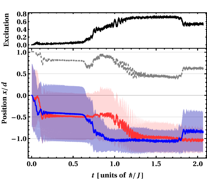
Figure 5: (color online) Time dependent behavior for a linear inclination with a final perturbation $\hat{W}=4400\,J_{1}\hat{R}_{x}/d=0.6\,\hbar\omega_{1}\hat{R}_{x}/d$. Top: Total occupation probability of states above the first Bloch band. Bottom: Legend as in Fig. 4.

V.2 Harmonic perturbation

In experiments optical lattices are not infinite but the atoms are normally confined by an additional weak harmonic potential. In the following the effect of the sudden activation of such a harmonic potential $\hat{W}=A(\hat{x}_{1}^{2}+\hat{x}_{2}^{2})/d^{2}$ is studied. This perturbation does not break the symmetry of the potential and the mean position of the atoms remains at $x/d=0$. However, as one can see in Fig. 6 (a) for a certain strength of the harmonic perturbation the system oscillates between unbound states ($\sqrt{\left<\rho_{x}^{2}\right>}\approx d$) and repulsively bound states ($\sqrt{\left<\rho_{x}^{2}\right>}\approx 0.5d$) Winkler et al. (2006) that are in resonance. These oscillations are also visible in the uncertainty of the atoms’ positions. For an increased harmonic perturbation no repulsively bound state is in resonance with the unbound state. Hence, as shown in Fig. 6(b) the atoms oscillate predominantly between delocalized states and states localized at the central lattice site. Since the atoms repel each other, the oscillations are exactly opposing each other. The off-resonant coupling to the bound state leads to small and fast oscillations of the mean distance $\sqrt{\left<\rho_{x}^{2}\right>}$ between $0.8d$ and $1.0d$.

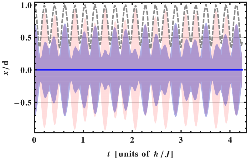
(a) x (b) x

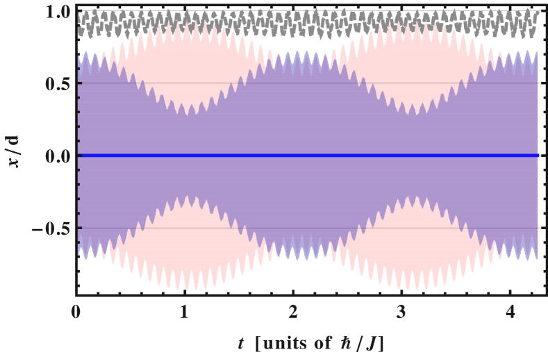
Figure 6: (color online) Time-dependent behavior for the sudden turn-on of an additional harmonic confinement. (a) For $\hat{W}=82\,J_{1}(\hat{x}_{1}^{2}+\hat{x}_{2}^{2})/d^{2}=0.01\,\hbar\omega_{1}(\hat{x}_{1}^{2}+\hat{x}_{2}^{2})/d^{2}$ oscillations between bound and unbound states appear. (b) For stronger confinement $\hat{W}=164\,J_{1}(\hat{x}_{1}^{2}+\hat{x}_{2}^{2})/d^{2}=0.02\,\hbar\omega_{1}(\hat{x}_{1}^{2}+\hat{x}_{2}^{2})/d^{2}$ the bound-state occupation is much weaker, however the particles tunnel alternating between the central and outer wells. Legend as in Fig. 4.

VI Conclusion and outlook

A theoretical approach for the full non-perturbative time-dependent description of two interacting particles in an optical lattice was introduced. A comparison with analytical results shows the possibility to perform high-precision analyses. Example calculations for ⁶Li-⁷Li in a three-well optical lattice where performed, demonstrating the possibility to analyze this complex six-dimensional system in terms of several expectation values. It was shown how the atoms are separated by a slowly increasing acceleration of the system and how the system reacts upon suddenly stopping the acceleration. It was also demonstrated that a fast acceleration of the lattice leads to a strong occupation of states above the first Bloch band, which marks the break down of the usually adopted single-band Hubbard models. As finally shown, a weak harmonic perturbation can have an important impact if the system encounters a resonance between bound and unbound states.

The use of a spectral method, i. e. expanding the time-dependent wavefunction in a basis of eigenfunctions of some underlying Hamiltonian, offers a large degree of flexibility. For example, by modifying the underlying Hamiltonian the here-presented system of two neutral atoms can be easily generalized to other particles, such as ions, or dipoles. Also the external potential is flexible enough to describe a large class of systems like quantum dots or one- and two-dimensional optical traps. In the future we intend to analyse and develop with the presented procedure schemes for the fast and high-fidelity manipulation of small quantum systems.

References

- Anderson et al. (1995) M. H. Anderson, J. R. Ensher, M. R. Matthews, C. E. Wieman, and E. A. Cornell, Science 269, 198 (1995).
- Davis et al. (1995) K. B. Davis, M. O. Mewes, M. R. Andrews, N. J. van Druten, D. S. Durfee, D. M. Kurn, and W. Ketterle, Phys. Rev. Lett. 75, 3969 (1995).
- Greiner et al. (2002) M. Greiner, O. Mandel, T. Esslinger, T. Hänsch, and I. Bloch, Nature 415, 39 (2002).
- Bloch et al. (2008) I. Bloch, J. Dalibard, and W. Zwerger, Rev. Mod. Phys. 80, 885 (2008).
- Bakr et al. (2010) W. S. Bakr, A. Peng, M. E. Tai, R. Ma, J. Simon, J. I. Gillen, S. Fölling, L. Pollet, and M. Greiner, Science 329, 547 (2010).
- Weitenberg et al. (2011) C. Weitenberg, M. Endres, J. F. Sherson, M. Cheneau, P. Schausz, T. Fukuhara, I. Bloch, and S. Kuhr, Nature 471, 319 (2011).
- Serwane et al. (2011) F. Serwane, G. Zürn, T. Lompe, T. B. Ottenstein, A. N. Wenz, and S. Jochim, Science 332, 336 (2011).
- Bakr et al. (2011) W. S. Bakr, P. M. Preiss, M. E. Tai, R. Ma, J. Simon, and M. Greiner, Nature 480, 500 (2011).
- Schneider and Saenz (2012) P.-I. Schneider and A. Saenz, Phys. Rev. A 85, 050304 (2012).
- Anderlini et al. (2007) M. Anderlini, P. J. Lee, B. L. Brown, J. Sebby-Strabley, W. D. Phillips, and J. V. Porto, Nature 448, 452 (2007).
- Trotzky et al. (2008) S. Trotzky, P. Cheinet, S. Fölling, M. Feld, U. Schnorrberger, A. M. Rey, A. Polkovnikov, E. A. Demler, M. Lukin, and I. Bloch, Science 319, 295 (2008).
- Wirth et al. (2010) G. Wirth, M. Ölschläger, and A. Hemmerich, Nature Physics 7, 147 (2010).
- Ivanov et al. (2008) V. V. Ivanov, A. Alberti, M. Schioppo, G. Ferrari, M. Artoni, M. L. Chiofalo, and G. M. Tino, Phys. Rev. Lett. 100, 043602 (2008).
- Sias et al. (2008) C. Sias, H. Lignier, Y. P. Singh, A. Zenesini, D. Ciampini, O. Morsch, and E. Arimondo, Phys. Rev. Lett. 100, 040404 (2008).
- Schneider et al. (2008) U. Schneider, L. Hackermüller, S. Will, T. Best, I. Bloch, T. A. Costi, R. W. Helmes, D. Rasch, and A. Rosch, Science 322, 1520 (2008).
- Busch et al. (1998) T. Busch, B.-G. Englert, K. Rzazewski, and M. Wilkens, Found. Phys. 28, 549 (1998).
- Schneider et al. (2011) P.-I. Schneider, Y. V. Vanne, and A. Saenz, Phys. Rev. A 83, 030701 (2011).
- Grishkevich et al. (2011) S. Grishkevich, S. Sala, and A. Saenz, Phys. Rev. A 84, 062710 (2011).
- Bandyopadhyay and Dattagupta (2008) M. Bandyopadhyay and S. Dattagupta, Pramana-Journal of Physics 70, 381 (2008).
- Winkler et al. (2006) K. Winkler, G. Thalhammer, F. Lang, R. Grimm, J. Hecker-Denschlag, A. J. Daley, A. Kantian, H. P. Büchler, and P. Zoller, Nature 441, 853 (2006).