Stern-Gerlach Effect of Weak-Light Ultraslow Vector Solitons

Abstract

We propose a scheme to exhibit Stern-Gerlach (SG) deflection of high-dimensional vector optical soliton (VOS) at weak-light level in a cold atomic gas via electromagnetically induced transparency. We show that the propagating velocity and generation power of such VOS can be reduced to $10^{-6}\,\,c$ ($c$ is light speed in vacuum) and lowered to magnitude of nanowatt, respectively. The stabilization of the VOS may be realized by using an optical lattice formed by a far-detuned laser field, and its trajectory can be deflected significantly by using a SG magnetic field. Deflection angle of the VOS can be of magnitude of $10^{-3}$ rad when propagating several millimeters. Different from atomic SG deflection, deflection angle of the VOS can be distinct for different polarization components and can be manipulated in a controllable way. The results obtained can be described in terms of a SG effect for the VOS with quasispin and effective magnetic moment.

Stern-Gerlach (SG) effect, i.e., a particle with nonzero magnetic moment deflects when passing through an inhomogeneous magnetic field, was firstly discovered in early time of quantum mechanics. This effect illustrates the necessity for a radical departure from classical mechanics, and characterizes quantum nature of atomic motion in a simple and fundamental way sak . Recently, similar effect was also predicted in many other systems, e.g., spinor Fermi and Bose gases GO and chiral molecules LBS .

All massive elementary particles, such as electrons, have non-zero magnetic moments. Contrarily, photons have no magnetic moment in vacuum, thus experience no force when passing through inhomogeneous magnetic field. Recently, in a very remarkable experiment KW , Karpa and Weitz showed that photons may acquire effective magnetic moments when propagating in a resonant atomic gas, and hence can deflect by a gradient magnetic field. In their experiment, a technique of electromagnetically induced transparency (EIT) fle is exploited, by which a small absorption and slow propagating velocity of photons can be realized.

However, the EIT-enhanced deflection of light in Ref. KW cannot be explained as a standard SG effect because only one component of “spin” is involved. In this Letter, we propose a double EIT scheme to demonstrate a SG effect of high-dimensional vector optical soliton (VOS), which not only has two polarization components (i.e. a quasispin) but also allows a distortionless propagation. Propagating velocity and generation power of the VOS can be reduced to very low level. Stabilization of the VOS can be realized using an optical lattice formed by a far-detuned laser field. The VOS can acquire very large effective magnetic moments, and the deflection of its trajectory is much more significant when passing though a SG gradient magnetic field.

Before proceeding, we note that besides Ref. KW , optical beam deflection in external fields has been the subject of many previous works SW ; hol ; PUR ; ZLZS ; GZKS . The present work is related to Refs. KW ; ZLZS ; GZKS and to recent studies of slow-light solitons WD ; HDP ; MPP . Essence of Refs. KW ; ZLZS ; GZKS is a SG effect of linear polaritons. However, such linear polaritons spread and attenuate during propagation because of the existence of diffraction and other detrimental effects. In Refs. WD ; HDP ; MPP , slow-light solitons via EIT are suggested, but no SG effect is considered.

In contrast, the scheme presented here exploits optical lattice and EIT-enhanced Kerr effect, which allow the formation and stable propagation of high-dimensional VOS, or called nonlinear polariton, with effective magnetic moment (SG deflection) being four (two) orders of magnitude larger than that of the linear polariton of Ref. KW . Thus, comparing with that obtained in a linear scheme KW ; ZLZS ; GZKS , the SG effect proposed here is more efficient and robust for observation and practical applications.

To be specific, we consider a medium consisting of five-level atoms with M-configuration. A linearly polarized, pulsed probe field (with pulse duration $\tau_{0}$) ${\bf E}_{p}={\bf E}_{p1}+{\bf E}_{p2}=({\bf\hat{\epsilon}}_{-}{\cal E}_{p1}+{\bf\hat{\epsilon}}_{+}{\cal E}_{p2})\exp[i(k_{p}z-\omega_{p}t)]+{\rm c.c.}$ drives the transitions $|3\rangle\leftrightarrow|2\rangle$ and $|3\rangle\leftrightarrow|4\rangle$ by its left-circular (i.e. $\sigma^{-}$) polarization component ${\bf E}_{p1}$ and right-circular (i.e. $\sigma^{+}$) polarization component ${\bf E}_{p2}$, respectively. Here ${\cal E}_{p1,p2}$ are envelopes and ${\bf\hat{\epsilon}}_{\pm}\equiv({\bf\hat{x}}\pm i{\bf\hat{y}})/\sqrt{2}$. A $\pi$-polarized, strong continuous-wave control field ${\bf E}_{c1}={\bf\hat{z}}{\cal E}_{c1}\exp[i(k_{c1}x-\omega_{c1}t)]+{\rm c.c.}$ (${\bf E}_{c2}={\bf\hat{z}}{\cal E}_{c2}\exp[i(k_{c2}x-\omega_{c2}t)]+{\rm c.c.}$) drives the transition $|1\rangle\leftrightarrow|2\rangle$ ($|5\rangle\leftrightarrow|4\rangle$) (Fig. 1(a) ). $\hat{\bf x}$, $\hat{\bf y}$, and $\hat{\bf z}$ are unit vectors along coordinate axes $x$, $y$ and $z$, respectively (Fig. 1(b)).

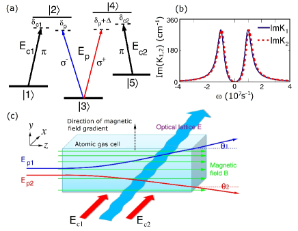
Figure 1: (color online) (a): Double EIT scheme. ${\bf E}_{p}$ and ${\bf E}_{cj}$ ($j=1,2$) are probe and control fields, respectively; $\delta_{p}$, $\delta_{p}+\Delta$, and $\delta_{cj}$ are detunings. (b): Absorption spectrum Im$K_{j}(\omega)$ as functions of $\omega$. Solid and dotted lines correspond to the $\sigma^{-}$ and $\sigma^{+}$ polarization components, respectively. (c): A possible experimental arrangement, where an inhomogeneous magnetic field ${\bf B}$ removes the degeneracy of ground states $|j\rangle$ ($j=1,3,5$) and excited states $|l\rangle$ ($l=2,4$), and causes Stern-Gerlach deflection of probe-field components. $\theta_{1}$ and $\theta_{2}$ are deflection angles of $\sigma^{-}$ polarization component (i.e. ${\bf E}_{p1}$) and $\sigma^{+}$ polarization component (i.e. ${\bf E}_{p2}$) of high-dimensional VOS, which has a quasispin and an effective magnetic moment. The curved thick arrow represents the far-detuned optical lattice field ${\bf E}$ used to stabilize the VOS.

We assume an inhomogeneous magnetic field ${\bf B}(y)=\hat{\bf z}B(y)=\hat{\bf z}(B_{0}+B_{1}y)$ ($B_{1}\ll B_{0}$) is applied to the system. Here $B_{0}$ contributes to a Zeeman level shift $\Delta E_{\rm Z}=\mu_{B}g_{F}^{j}m_{F}^{j}B_{0}$, and hence removes the degeneracy of ground-state sublevels $|j\rangle$ ($j=1,3,5$) and the excited-state sublevels $|l\rangle$ ($l=2,4$). $\mu_{B}$, $g_{F}^{j}$, and $m_{F}^{j}$ are Bohr magneton, gyromagnetic factor, and magnetic quantum number of the level $|j\rangle$, respectively. $B_{1}$ contributes a transverse gradient of the magnetic field, resulting in a SG deflection of the probe field.

We assume further a small, far-detuned laser field ${\bf E}(x,t)=\hat{\bf x}E_{0}\cos(x/R_{\perp})\cos(\omega_{L}t)$ is also applied into the medium, where $E_{0}$, $R_{\perp}$, and $\omega_{L}$ are field amplitude, beam radius, and angular frequency, respectively. Due to ${\bf E}(x,t)$, Stark level shift $\Delta E_{j,\rm S}=-\frac{1}{2}\alpha_{j}\langle E^{2}\rangle_{t}=-\frac{1}{2}\alpha_{j}E^{2}(x)$ occurs, here $\alpha_{j}$ is the scalar polarizability of the level $|j\rangle$, $\langle\cdots\rangle_{t}$ denotes the time average in an oscillation cycle, and hence $E(x)=(E_{0}/\sqrt{2})\cos(x/R_{\perp})$. The aim of introducing the far-detuned laser field is to form an optical lattice potential to stabilize the high-dimensional VOS BMS , as shown below.

Besides, atoms are assumed prepared initially in the ground-state level $|3\rangle$ and trapped in a gas cell with ultracold temperature to cancel Doppler broadening and collisions. Thus, the system is composed of two $\Lambda$-type EIT configurations (i.e. double EIT). A possible arrangement of experimental apparatus is suggested in Fig. 1(c).

Under electric-dipole and rotating-wave approximations, the Hamiltonian of the system in interaction picture is $H_{\rm int}/\hbar=(\delta_{p}-\delta_{c1})|1\rangle\langle 1|+\delta_{p}|2\rangle\langle 2|+(\delta_{p}+\Delta)|4\rangle\langle 4|+(\delta_{p}+\Delta-\delta_{c2})|5\rangle\langle 5|+\Omega_{c1}|2\rangle\langle 1|+\Omega_{p1}|2\rangle\langle 3|+\Omega_{p2}|4\rangle\langle 3|+\Omega_{c2}|4\rangle\langle 5|+{\rm H.c.}$, where $\Omega_{p1}$=$-(\textbf{p}_{23}\cdot\hat{{\bf\epsilon}}_{-}){\cal E}_{p1}/\hbar$ and $\Omega_{p2}$=$-(\textbf{p}_{43}\cdot\hat{{\bf\epsilon}}_{+}){\cal E}_{p2}/\hbar$ ($\Omega_{c1}$=$-(\textbf{p}_{21}\cdot\hat{\bf z}){\cal E}_{c1}/\hbar$ and $\Omega_{c2}$=$-(\textbf{p}_{45}\cdot\hat{\bf z}){\cal E}_{c2}/\hbar$) are respectively Rabi frequencies of two circularly polarized components of the probe field (two $\pi$-polarized control fields), with $\textbf{p}_{jl}$ being the electric dipole matrix element associated with the transition from $|j\rangle$ to $|l\rangle$. The detunings are defined as $\delta_{p}=\omega_{23}+\mu_{23}B(y)-\frac{1}{2}\alpha_{23}E(x)^{2}-\omega_{p}$, $\delta_{c1}=\omega_{21}+\mu_{21}B(y)-\frac{1}{2}\alpha_{21}E(x)^{2}-\omega_{c1}$, $\delta_{c2}=\omega_{45}+\mu_{45}B(y)-\frac{1}{2}\alpha_{45}E(x)^{2}-\omega_{c2}$, and $\Delta=\mu_{42}B(y)-\frac{1}{2}\alpha_{42}E(x)^{2}$, where $\mu_{jl}=\mu_{B}(g_{F}^{j}m_{F}^{j}-g_{F}^{l}m_{F}^{l})/\hbar$, $\alpha_{jl}=(\alpha_{j}-\alpha_{l})/\hbar$, and $\omega_{jl}=(E_{j}-E_{l})/\hbar$, with $E_{j}$ being the eigenenergy of the state $|j\rangle$.

The motion of atoms is governed by the Bloch equation for density-matrix $\rho$,

$$\partial\rho/\partial t=-i[H_{\rm int},\rho]/\hbar-\Gamma(\rho),$$ (1)

where $\Gamma(\rho)$ is relaxation matrix representing spontaneous emission and dephasing (see Supplementary Material). Electric-field evolution is controlled by Maxwell equation

$$\nabla^{2}\textbf{E}-(1/c^{2})\partial^{2}\textbf{E}/\partial t^{2}=(1/\epsilon_{0}c^{2})\partial^{2}\textbf{P}/\partial t^{2},$$ (2)

where $\textbf{P}={\cal N}{\rm Tr}({\bf p}\rho)$ is electric polarization with ${\cal N}$ the atomic density. Under slowly varying envelope approximation, Eq. (2) reduces to $[i\partial_{z}+(i/c)\partial_{t}+c\nabla_{\perp}^{2}/(2\omega_{p})]\Omega_{p1,p2}-\kappa_{32,34}\rho_{23,43}=0$, where $\nabla_{\perp}^{2}=\partial^{2}/\partial x^{2}+\partial^{2}/\partial y^{2}$ and $\kappa_{32,34}={\cal N}|\textbf{p}_{32,34}\cdot{\bf\hat{\epsilon}}_{\mp}|^{2}\omega_{p}/(2\hbar\epsilon_{0}c)$ with $\epsilon_{0}$ the vacuum dielectric constant.

Linear propagation of the probe field in the absence of diffraction can be obtained by taking $\Omega_{p1,p2}$ as small quantities and $B_{1}$, $E_{0}$ as zero. Then one has $\Omega_{pj}=F_{j}\exp\{i[K_{j}(\omega)z-\omega t)]\}$ ($j=1,2$) with $K_{1,2}(\omega)=\omega/c+\kappa_{32,34}(\omega-d_{1,5})/D_{1,2}$ (linear dispersion relation). Here, $F_{j}$ are constants, $D_{1,2}=|\Omega_{c1,c2}|^{2}-(\omega-d_{1,5})(\omega-d_{2,4})$, $d_{1}=(\delta_{p}-\delta_{c1})-i\gamma_{13}/2$, $d_{2}=\delta_{p}-i(\Gamma_{2}+\gamma_{23})/2$, $d_{4}=(\delta_{p}+\Delta)-i(\Gamma_{4}+\gamma_{34})/2$, and $d_{5}=(\delta_{p}+\Delta-\delta_{c2})-i\gamma_{35}/2$ with $\delta_{p}=\omega_{23}+\mu_{23}B_{0}-\omega_{p}$, $\Delta=\mu_{42}B_{0}$, $\delta_{c1}=\omega_{21}+\mu_{21}B_{0}-\omega_{c1}$, and $\delta_{c2}=\omega_{45}+\mu_{45}B_{0}-\omega_{c2}$. $\Gamma_{i}$ and $\gamma_{ij}$ denote the spontaneous emission and dephasing rates of relevant states, respectively.

The linear dispersion relation displays two branches. Fig. 1(b) shows the absorption spectrum of Im$K_{j}(\omega)$ ($j=1,2$) as a function of frequency $\omega$. Parameters are chosen for a laser-cooled ⁸⁵Rb atomic gas with $|1\rangle=|5^{2}S_{1/2},F=2,m_{F}=-1\rangle$, $|2\rangle=|5^{2}P_{1/2},F=2,m_{F}=-1\rangle$, $|3\rangle=|5^{2}S_{1/2},F=1,m_{F}=0\rangle$, $|4\rangle=|5^{2}P_{1/2},F=2,m_{F}=1\rangle$, and $|5\rangle=|5^{2}S_{1/2},F=2,m_{F}=1\rangle$. Decay rates are $\Gamma_{2}\simeq\Gamma_{4}\simeq 6$ MHz and $\gamma_{13}\simeq\gamma_{23}\simeq\gamma_{34}\simeq\gamma_{35}\simeq 50$ Hz. Other parameters are taken as $\kappa_{32}\simeq\kappa_{34}=1.0\times 10^{9}$ cm^-1s^-1, $\Omega_{c1}=\Omega_{c2}=1.0\times 10^{7}$ s^-1, $\delta_{p}=\delta_{c1}=\delta_{c2}=0$, and $B_{0}=34.1$ mG. The solid (dotted) line in the figure is for $\sigma^{-}$ ($\sigma^{+}$) polarization component. We see that large and deep transparency windows in the absorption spectra of both polarization components (double EIT) appear. Using above parameters, group velocities of the both components (defined by $V_{gj}={\rm Re}(\partial K_{j}/\partial\omega)^{-1}$) are given as $3.3\times 10^{-6}c$.

However, the linear solution is unstable due to the diffraction and other detrimental effects, which results in spreading and attenuation of the probe field during propagation, as demonstrated by Eq. (24) of Ref. GZKS . To solve this problem we use nonlinear effect to suppress the spreading and attenuation. When including weak nonlinearity and diffraction, we obtain the following nonlinearly coupled, dimensionless equations, derived by using a standard method of multiple-scales (see the Supplementary Material):

$$\left[\frac{i}{v_{g1,g2}}\frac{\partial}{\partial\tau}+\frac{1}{2}\left(\frac{\partial^{2}}{\partial\xi^{2}}+\frac{\partial^{2}}{\partial\eta^{2}}\right)\right]u_{1,2}-\frac{1}{\sqrt{2\pi}\rho_{0}}(g_{11,22}|u_{1,2}|^{2}$$

$$+g_{12,21}|u_{2,1}|^{2})u_{1,2}+V_{1,2}(\xi,\eta)u_{1,2}=-iA_{1,2}u_{1,2}.$$ (3)

where $\tau$=$t/\tau_{0}$, $(\xi,\eta)$=$(x,y)/R_{\bot}$, $v_{gj}$=$V_{gj}\tau_{0}/L_{\rm Diff}$, and $u_{j}(\tau,\xi,\eta)$=$[\Omega_{pj}/F_{j}(\rho_{j})]e^{-i{\rm Re}[K_{j}|_{\omega=0}]z}/U_{0}$. Here, $L_{\rm Diff}=\omega_{p}R_{\bot}^{2}/c$ and $U_{0}$ are respectively the typical diffraction length and Rabi frequency, $F_{j}(\rho_{j})$ are normalized Gaussian functions (i.e. $F_{j}=[1/(\rho_{0}\sqrt{\pi})]^{1/2}\exp[-\rho_{j}^{2}/(2\rho_{0}^{2})]$ with $\rho_{j}=(z-V_{gj}t)/L_{\rm Diff}$ and $\rho_{0}$ a constant GZKS ), $g_{11,12,21,22}=W_{11,12,21,22}/|W_{22}|$ are nonlinearity coefficients with $W_{11,22}=-\kappa_{32,34}d_{1,5}(|d_{1,5}|^{2}+|\Omega_{c1,c2}|^{2})/(D_{1,2}|D_{1,2}|^{2})$ and $W_{12,21}=-\kappa_{32,34}d_{1,5}(|d_{5,1}|^{2}+|\Omega_{c2,c1}|^{2})/(D_{1,2}|D_{2,1}|^{2})$ characterizing respectively self-phase and cross-phase modulations, and $A_{j}$=${\rm Im}[K_{j}|_{\omega=0}]L_{\rm Diff}$ are small absorption coefficients.

Combined potentials in Eq. (Stern-Gerlach Effect of Weak-Light Ultraslow Vector Solitons) have the form

$$V_{j}(\xi,\eta)={\cal M}_{j}\eta+{\cal N}_{j}\cos^{2}(\xi),$$ (4)

where ${\cal M}_{1,2}=M_{1,2}R_{\bot}B_{1}$ and ${\cal N}_{1,2}=N_{1,2}E_{0}^{2}$ are contributions from the SG gradient magnetic field (proportional to $B_{1}$) and the optical lattice field (proportional to $E_{0}^{2}$), respectively. $M_{j}$ and $N_{j}$ are defined as $M_{1,2}$= $-\kappa_{32,34}(d_{1,5}^{2}\mu_{23,43}+|\Omega_{c1,c2}|^{2}\mu_{13,53})L_{\rm Diff}/D_{1,2}^{2}$ and $N_{1,2}$=$\frac{1}{4}\kappa_{32,34}(d_{1,5}^{2}\alpha_{23,43}+|\Omega_{c1,c2}|^{2}\alpha_{13,53})L_{\rm Diff}/D_{1,2}^{2}$. When deriving Eq. (Stern-Gerlach Effect of Weak-Light Ultraslow Vector Solitons), $B_{1}$ and $E_{0}^{2}$ are assumed as small quantities. Additionally, $\tau_{0}$ is also assumed to be large (e.g. $\tau_{0}=2.1$ $\mu$s) so that the second-order dispersion (proportional to $\partial^{2}u_{j}/\partial\tau^{2}$) is negligible.

Fig. 2 (a) and (b) show

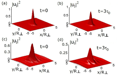
Figure 2: (color online) (a) and (b): Evolutions of $|u_{1}|^{2}$ respectively at $t=0$ and $t=3\tau_{0}$ for single-peaked VOS. (c) and (d): Evolutions of $|u_{1}|^{2}$ respectively at $t=0$ and $t=3\tau_{0}$ for multiple-peaked VOS. SG gradient magnetic field is absent (i.e. $B_{1}=0$). The stability of the VOS is achieved by the far-detuned optical lattice. Result for $|u_{2}|^{2}$ is similar to $|u_{1}|^{2}$ thus not shown.

results of numerical simulation for $|u_{1}|^{2}$ respectively at $t=0$ and $t=3\tau_{0}$ for a deep optical lattice ($E_{0}=3.2\times 10^{4}$ V cm^-1). The soliton obtained displays a single-peaked structure. The result for $|u_{2}|^{2}$ is similar to $|u_{1}|^{2}$ due to symmetry and hence not shown. The case for a shallower optical lattice ($E_{0}=2.3\times 10^{4}$ V cm^-1) is also simulated, with the result plotted in panels (c) and (d) for $t=0$ and $t=3\tau_{0}$, respectively. We see that in this case a multiple-peaked soliton appears. In both simulations, $\delta_{p}=1.0\times 10^{6}$ s^-1, $\delta_{c2}=1.0\times 10^{5}$ s^-1, and $R_{\perp}=16$ $\mu$m with other parameters the same with those in Fig. 1. In addition, $U_{0}=6.8\times 10^{6}$ s^-1, which allows enough nonlinearity to balance the diffraction. The typical diffraction length $L_{\rm Diff}$ and nonlinearity length $L_{\rm Nonl}$ ($\equiv 1/(U_{0}^{2}|W_{22}|$) are $\simeq 0.2$ cm. Furthermore, $B_{1}$ is chosen as zero, i.e., the SG gradient magnetic field is absent, thus no SG deflection occurs.

The stability of the high-dimensional VOS is checked by adding a small random perturbation to the stationary solution obtained in imaginary time (Fig. 2 (a), (c)) and evolving the solution according to Eq. (Stern-Gerlach Effect of Weak-Light Ultraslow Vector Solitons) in real time. We find that the soliton can indeed propagate stably for a long time (Fig. 2 (b), (d)). We have also used a standard linear stability analysis (see the Supplementary Material) to confirm the stability of the high-dimensional VOS.

Next we study VOS deflection by numerically simulating Eq. (Stern-Gerlach Effect of Weak-Light Ultraslow Vector Solitons) with $B_{1}\neq 0$. Shown in Fig. 3

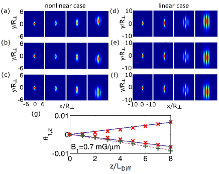
Figure 3: (color online) SG effect of ultraslow VOS. (a) and (b): Symmetric deflection (on $y$-axis) of $|u_{1}|^{2}$ and $|u_{2}|^{2}$ when propagating from $z=2L_{\rm Diff}$ to $z=8L_{\rm Diff}$ (corresponding respectively to the subfigure from left to right), respectively. (c): Asymmetric deflection of $|u_{2}|^{2}$ ($|u_{1}|^{2}$ is the same as (a) thus not shown). (d), (e), (f): Corresponding evolution of linear polariton. (g): Deflection angles of the VOS as functions of $z/L_{\rm Diff}$ for $B_{1}=0.7$ mG/$\mu$m. The solid line with positive (negative) slope is the analytical result of $\theta_{1}$ ($\theta_{2}$) for the symmetric case. Dashed line is the analytical result of $\theta_{2}$ for the asymmetric case ($\theta_{1}$ is the same as the symmetric case thus not shown). Points labeled by “x” and “+” are center positions of the VOS polarization components obtained numerically.

(a) and (b) are spatial distributions of $|u_{1}|^{2}$ (panel (a)) and $|u_{2}|^{2}$ (panel (b)) in ($x,y$)-plane when the VOS propagates from $z=2L_{\rm Diff}$ to $z=8L_{\rm Diff}$ with group velocity $V_{g1}\simeq V_{g2}=3.2\times 10^{-6}c$. In the simulation, $B_{1}=0.7$ mG $\mu$m^-1 is chosen. We see that an obvious deflection of VOS trajectories occurs due to the existence of the SG gradient magnetic field. Additionally, two different polarization components deflect symmetrically in $+y$ and $-y$ directions, similar to the SG deflection for atoms.

The SG deflection of VOS components can be made asymmetric. To show this, we take $\Omega_{c2}=0.9\times 10^{7}$ s^-1 without changing other parameters, then $(V_{g1},V_{g2})=(3.2,2.6)\times 10^{-6}c$. As a result, the trajectory of $\sigma^{-}$ component keeps unchanged, whereas the trajectory of $\sigma^{+}$ component changes as shown in Fig. 3(c). This is different from atomic SG deflection, where trajectories are always symmetric for two different spin components.

For comparison, in Fig. 3(d), (e), and (f) we present results of corresponding evolution for a linear polariton. One sees that the probe pulse spread rapidly. Thus the nonlinear effect is necessary for obtaining stable VOS and its robust SG deflection.

Analytical VOS solutions of Eq. (Stern-Gerlach Effect of Weak-Light Ultraslow Vector Solitons) can be gained under some approximations: (i)The small absorption term $-iA_{j}u_{j}$ is disregarded. (ii)Since in the presence of the SG gradient magnetic field the two polarization components of VOS separate each other after propagating some distance, the cross-phase-modulation terms can be neglected. (iii)The optical lattice is deep enough so that $V_{j}$ can be approximated as ${\cal M}_{j}\eta+{\cal N}_{j}(1-\xi^{2})$. Taking $u_{j}(\tau,\xi,\eta)=w_{j}(\tau,\eta)\phi_{j}(\xi)\exp[i{\cal N}_{j}v_{gj}\tau]$, where $\phi_{j}(\xi)$ is the normalized ground state of the eigenvalue problem $(\partial^{2}/\partial\xi^{2}-2{\cal N}_{j}\xi^{2})\phi_{j}=2E_{\xi}\phi_{j}$ with $E_{\xi}=-\sqrt{{\cal N}_{j}/2}$, and integrating out the variable $\xi$, Eq. (Stern-Gerlach Effect of Weak-Light Ultraslow Vector Solitons) reduces to $[(i/v_{gj})\partial_{\tau}+(1/2)\partial^{2}_{\eta}]w_{j}-{\cal N}_{j}^{1/4}/(2^{3/4}\pi\rho_{0})g_{jj}|w_{j}|^{2}w_{j}+({\cal M}_{j}\eta-\sqrt{{\cal N}_{j}/2})w_{j}=0$, which admits exact soliton solutions YZY . A single-soliton solution (see the Supplementary Material) gives

$$\Omega_{pj}= U_{0}A_{j}\,[1/(\rho_{0}\sqrt{\pi})]^{1/2}\,(\sqrt{2{\cal N}_{j}}/\pi)^{1/4}e^{i\varphi_{j}}$$ (5)

$$\times e^{-(s-v_{gj}\tau)^{2}/(2\rho_{0}^{2})}\,e^{-\sqrt{{\cal N}_{j}}\xi^{2}/\sqrt{2}}{\rm sech}\Theta_{j},$$

where $A_{j}=(2^{5/4}{\cal N}_{j}^{1/4}\pi\rho_{0}/|g_{jj}|)^{1/2}$, $\varphi_{j}={\cal M}_{j}v_{gj}\tau(\eta-{\cal M}_{j}v_{gj}^{2}\tau^{2}/6)$, and $\Theta_{j}=(2{\cal N}_{j})^{1/4}(\eta-{\cal M}_{j}v_{gj}^{2}\tau^{2}/2)$ ($j=1,2$). We see that both VOS components are localized in three spatial and one temporal dimensions. Thus, $(u_{1},u_{2})$ can be considered as a vector light bullet.

After passing the medium with length $L$, the center position of the $j$th polarization component of the VOS is at $(x,y_{j},z)$=$(0,{\cal M}_{j}L^{2}R_{\bot}/(2L_{\rm diff}^{2}),L)$, with the propagating velocity along the $z$- ($y$-) direction given by $V_{gj}$ ($V_{j}\equiv{\cal M}_{j}v_{gj}^{2}R_{\bot}t/\tau_{0}^{2})$. As a result, the expected deflection angle of the $j$th VOS component is

$$\theta_{j}=V_{j}/V_{gj}=(L/V_{gj})(\mu_{{\rm sol}\,j}/p)r^{2}B_{1},$$ (6)

where $r=R_{\bot}/L_{\rm Diff}$, $p=\hbar k_{p}$ is photon momentum, $\mu_{{\rm sol}\,j}=M_{j}V_{gj}\hbar k_{p}$ is effective magnetic moment. With the data in Fig. 3, we obtain $\mu_{{\rm sol}\,1,2}=\pm 7.6\times 10^{-20}$ J/T, which is four orders of magnitude larger than the effective magnetic moment for linear polariton of Ref. KW . From Eq. (6) we see the deflection angle of the $j$th polarization component of the VOS is proportional to the medium length $L$, the SG gradient magnetic field $B_{1}$, and inversely proportional to the group velocity $V_{gj}$. In a mechanical viewpoint, the deflection of the $j$th component of the VOS is caused by the transverse magnetic force $F_{j}=\mu_{{\rm sol}\,j}B_{1}$ and deflection angles can be expressed as $\theta_{j}=F_{j}t_{{\rm int}\,j}r^{2}/p_{j}$ with $t_{{\rm int}\,j}=L/V_{gj}$ being the interaction time. Due to untraslow propagating velocity, large deflection angles may be observed even for small $L$.

Fig. 3(g) shows deflection angles of the VOS as functions of $z/L_{\rm Diff}$ for $B_{1}=0.7$ mG/$\mu$m. The solid line of positive (negative) slope is the analytical result of $\theta_{1}$ ($\theta_{2}$) by Eq. (6) for the $\sigma^{-}$ ($\sigma^{+}$) component with $V_{g1}\simeq V_{g2}=3.3\times 10^{-6}c$ (i.e. the symmetric case). Points labeled by “x” are center positions of the VOS components obtained numerically. We thus have $(\theta_{1},\theta_{2})\simeq(1.6,-1.6)\times 10^{-3}$ rad for $z=0.4$ cm, which is two orders of magnitude larger than that for linear polariton obtained in Ref. KW . The dashed line is the analytical result of $\theta_{2}$ with $(V_{g1},V_{g2})=(3.2,2.6)\times 10^{-6}c$ (i.e. the asymmetric case) and points labeled by “+” are numerical results ($\theta_{1}$ is the same as the symmetric case). In both cases analytical results agree well with numerical ones.

The generation power of the high-dimensional VOS predicted above can be estimated by using Poynting’s vector HDP , which is $3.5$ nW calculated using the above parameters. Thus, very low input power is needed for generating the VOS in the present double EIT system.

In conclusion, a scheme is proposed to exhibit SG deflection of high-dimensional VOS via a double EIT. The VOS has ultraslow propagating velocity and extremely low generation power. The stabilization of the VOS can be realized by using an optical lattice, and its trajectory can be significantly deflected by a SG gradient magnetic field. The results obtained can be described in terms of a SG effect of the VOS with quasispin and effective magnetic moments. We expect that such large and robust SG effect may have potential applications in magnetometery and quantum information processing.

This work was supported by the NSF-China under Grant Nos. 11174080 and 11105052.

References

• (1) J. J. Sakurai, Modern Quantum Mechanics (Revised Edition) (Addison-Wesley, 1994).
• (2) M. D. Girardeau and M. Olshanii, Phys. Rev. A 70, 023608 (2004).
• (3) Y. Li et al., Phys. Rev. Lett. 99, 130403 (2007).
• (4) L. Karpa and M. Weitz, Nat. Phys. 2, 332 (2006).
• (5) M. Fleischhauer et al., Rev. Mod. Phys. 77, 633 (2005).
• (6) R. Schlesser and A. Weis, Opt. Lett. 17, 1015 (1992).
• (7) R. Holzner et al., Phys. Rev. Lett. 78, 3451 (1997).
• (8) G. T. Purves et al., Eur. Phys. J. D 29, 433 (2004).
• (9) D. L. Zhou et al., Phys. Rev. A 76, 055801 (2007).
• (10) Y. Guo et al., Phys. Rev. A 78, 013833 (2008).
• (11) Y. Wu and L. Deng, Phys. Rev. Lett. 93, 143904 (2004).
• (12) G. Huang et al., Phys. Rev. E 72, 016617 (2005).
• (13) H. Michinel et al., Phys. Rev. Lett. 96, 023903 (2006).
• (14) B. B. Baizakov et al., Phys. Rev. A 70, 053613 (2004).
• (15) J. Yan et al., Phys. Fluids A 4, 690 (1992).