NLO QCD corrections to multi-jet production at the LHC with a centre-of-mass energy of $\sqrt{s}=8$ TeV

Abstract

We study three and four jet production in hadronic collisions at next-to-leading order accuracy in massless QCD. We cross check results previously obtained by the BlackHat collaboration for the LHC with a centre-of-mass energy of $\sqrt{s}=7$ TeV and present new results for the LHC operating at 8 TeV. We find large negative NLO corrections reducing the leading-order cross sections by about 40–50%. Furthermore we observe an important reduction of the scale uncertainty. In addition to the cross sections we also present results for differential distributions. The dynamical renormalization/factorization scale used in the calculation leads to a remarkably stable K-factor. The results presented here were obtained with the NJet package [1], a publicly available library for the evaluation of one-loop amplitudes in massless QCD.
Draft from

1 Introduction

Multi-jet production in hadronic collisions via the strong interaction represents an important testing ground for quantum chromodynamics (QCD). Jet production in massless QCD may provide valuable information to constrain the QCD coupling constant $\alpha_{s}$ and/or the parton distribution functions (PDFs). Furthermore owing to their significant production rates multi-jet processes may contribute as background processes to a large variety of interesting signal reactions including processes relevant for new physics searches. Independent of whether multi-jet production in QCD is studied as signal or background process precise theoretical predictions are mandatory.

In the past substantial progress has been made in the numerical evaluation of leading order (LO) matrix elements for large multiplicities. Using publicly available tools like Alpgen [2], Sherpa+Comix [3, 4], MadGraph/MadEvent [5, 6, 7] and Helac [8] multiplicities with up to 12 final state jets can be calculated. However leading-order cross section predictions suffer from a substantial (residual) dependence on the unphysical renormalization scale $\mu_{r}$. This is in particular true for high multiplicities due to the high power in $\alpha_{s}$ occurring in the perturbative expansion. For a process starting with $\alpha_{s}^{n}$ the scale dependent terms are proportional to

$$n\beta_{0}\alpha_{s}\sigma_{0}$$ (1)

where $\sigma_{0}$ denotes the leading-order cross section and $\beta_{0}$ is the leading coefficient of the QCD beta function. Precise theoretical predictions thus require at least next-to-leading order (NLO) corrections in the coupling $\alpha_{s}$ to reduce the scale dependence. While the NLO corrections to two jet production were calculated already in 1992 [9, 10] and the corrections to three jet production a decade later [11, 12] (results for the gluon channel were obtained already in Refs. [13, 14]) further progress has been hindered by both the increasing complexity of the one-loop amplitudes and the large number of tree-level processes entering the infra-red counter-terms in the Catani-Seymour subtraction formalism [15]. The latter problem could be solved by an automated generation of subtraction terms based on the aforementioned tree-level technology [16, 17, 18, 19, 20, 21]. While technically solved the available computer resources still impose a severe restriction on the multiplicity which can be handled in practice. As far as the virtual corrections are concerned just the mere number of Feynman diagrams in the conventional Feynman diagram based approach e.g. $\sim 15,000$ for $gg\to 4g$ at one-loop (neglecting self-energy type corrections) shows that alternative techniques are required. In recent years new methods for the evaluation of one-loop amplitudes have relieved the long standing bottleneck in producing virtual corrections for processes with high parton multiplicities. The on-shell unitarity method [22, 23] and the subsequently developed generalized unitarity method [25, 26, 27, 28, 29, 24] offer an interesting alternative to conventional Feynman diagram based methods. In particular the unitarity method allows to use leading order amplitudes as basic building blocks for the one-loop calculation. It is thus possible to make use of the efficient tree-level machinery mentioned above. In parallel with the development of the unitarity method also the conventional approach has been continuously improved in the last couple of years and a mixture of methods are currently exploited [30]. We also mention that recently other directions have been investigated which offer the potential to become powerful alternatives to those above [31]. While improvements are still ongoing, NLO technology is already now automated and flexible enough to cover a wide range of processes for four final state particles [32, 33, 34, 35, 36, 37, 38, 39, 40, 41, 42, 43, 44, 45, 46, 47, 48, 49, 50, 51, 52] and a handful of $2\to\geq 5$ processes [53, 54, 55, 31]. A number of automated approaches to the computation of virtual amplitudes have appeared as public codes [56, 58, 57, 59].

Despite the aforementioned progress only very recently first results for four jet production in NLO accuracy became available. In Ref. [60] the BlackHat collaboration published results for three and four jet production in NLO accuracy for the LHC running at 7 TeV centre-of-mass energy. Given the complexity of the calculation it is very important to perform an independent cross check. Furthermore we present results for the LHC running at 8 TeV and discuss various differential distributions. For the evaluation of the virtual matrix elements we use the publicly available package NGluon [56]. NGluon uses on-shell methods to evaluate numerically one-loop primitive amplitudes in pure gauge theory. Recently we have extended NGluon to account for amplitudes involving massless quarks [61, 62, 1]. We note that in Refs. [61, 62, 1] no approximation in the colour is performed. The real corrections and the cancellation of soft- and collinear divergences are obtained within the Catani-Seymour dipole subtraction method [15]. For this contribution we use the Sherpa Monte-Carlo event generator [16]. We will briefly comment on some technical aspects in the next section. In section 3 we will present the comparison with the results published by BlackHat [60]. In addition we show new results for 8 TeV for three and four jet production. Our conclusions are presented in section 4.

2 Outline of the calculation

In what follows we briefly outline the calculation. We work in massless QCD with 5 flavours. In particular we include the bottom quark in the initial state. The top-quark is assumed to be integrated out. Through the matching of the coupling constants between the five and the six flavour theories some of the corrections due to top-quarks are retained. We expect the neglected corrections to be small. For three jet production the contributing processes are given by all possible crossings of the following transitions:

$$0\to ggggg,\quad 0\to q{\overline{q}}ggg,\quad 0\to q{\overline{q}}q^{\prime}{\overline{q}}^{\prime}g,$$ (2)

where $q$ and $q^{\prime}$ denote a generic quark. For the four jet production the corresponding processes are derived from

$$0\to gggggg,$$ (3)

and

$$0\to q{\overline{q}}gggg,\quad 0\to q{\overline{q}}q^{\prime}{\overline{q}}^{\prime}gg,\quad 0\to q{\overline{q}}q^{\prime}{\overline{q}}^{\prime}q^{\prime\prime}{\overline{q}}^{\prime\prime}.$$ (4)

In principle we need to distinguish the like-flavour cases from the case that all quark flavours are different. However technically the like-flavour processes can be obtained from the latter by an appropriate (anti) symmetrization with respect to the quark momenta. For example the amplitude $A_{q{\overline{q}}q{\overline{q}}g}$ for the transition $0\to q{\overline{q}}q{\overline{q}}g$ is obtained through

$$A_{q{\overline{q}}q{\overline{q}}g}(1,2,3,4,5) =$$ (5)

$$A_{q{\overline{q}}q^{\prime}{\overline{q}}^{\prime}g}(1,2,3,4,5)-A_{q{\overline{q}}q^{\prime}{\overline{q}}^{\prime}g}(1,4,3,2,5),$$

where we used the short hand notation to abbreviate with $i$ the momentum $k_{i}$ and helicity $\lambda_{i}$ of the $i$-th parton ($i=(k_{i},\lambda_{i})$). The expansion of the $n$-jet differential cross section in the coupling $\alpha_{s}$ reads:

$$d\sigma_{n}=d\sigma_{n}^{\mbox{\scriptsize LO}}+d\delta\sigma_{n}^{\mbox{\scriptsize NLO}}+{\cal O}(\alpha_{s}^{n+2})$$ (6)

($d\sigma_{n}^{\mbox{\scriptsize LO}}\sim\alpha_{s}^{n},d\delta\sigma_{n}^{\mbox{\scriptsize NLO}}\sim\alpha_{s}^{n+1}$) with the leading order cross section given by

$$d\sigma_{n}^{\mbox{\scriptsize LO}}= \sum_{\begin{subarray}{c}i,j\\ \in\{q,{\overline{q}},g\}\end{subarray}}dx_{i}dx_{j}F_{j/H_{2}}(x_{j},\mu_{f})F_{i/H_{1}}(x_{i},\mu_{f})$$

$${}\times d\sigma_{n}^{\rm B}\bigl{(}i(x_{i}P_{1})+j(x_{j}P_{2})\to n\mbox{ part.}\bigr{)}.$$ (7)

$P_{1},P_{2}$ denote the momenta of the incoming hadrons. $x_{i}$ are the momentum fractions carried by the initial state partons $i$ with respect to the incoming hadrons $H_{1},H_{2}$. The momentum sum of the incoming partons is thus given by $P=x_{i}P_{1}+x_{j}P_{2}$. As usual we neglect the masses of the incoming hadrons. $F_{i/H}(x_{i},\mu_{f})$ are the parton distribution functions which roughly speaking describe the probability to find a parton $i$ inside the hadron $H$ with a momentum fraction between $x_{i}$ and $x_{i}+dx_{i}$. The factorization scale is denoted by $\mu_{f}$. The partonic cross section for the reaction $(ij\to n\mbox{-jets})$ in Born approximation is given by $d\sigma_{n}^{B}\bigl{(}i(x_{1}P_{1})+j(x_{j}P_{2})\to n\mbox{-jets}\bigr{)}$. In terms of the leading order squared matrix elements $|{\cal M}_{n}|^{2}$ the explicit expression for $d\sigma_{n}^{B}$ reads:

$$d\sigma_{n}^{\rm B}=\frac{1}{2\hat{s}}\prod_{\ell=1}^{n}\frac{d^{3}k_{\ell}}{(2\pi)^{3}2E_{\ell}}\Theta_{n\text{-jet}}\\ {}\times(2\pi)^{4}\delta\Bigl{(}P-\sum_{m=1}^{n}k_{m}\Bigr{)}\big{|}{\cal M}_{n}(ij\to n\mbox{ part.})\big{|}^{2},$$ (8)

where $k_{i}$ are the four momenta of the outgoing partons and $\hat{s}=2x_{i}x_{j}(P_{1}\cdot P_{2})=(\sum_{i=1}^{n}k_{i})^{2}$ is the partonic centre of mass energy squared. The jet algorithm is encoded through $\Theta_{n\text{-jet}}$. $\Theta_{n\text{-jet}}$ is a function of the final state parton momenta $k_{i}$. It is one if the corresponding $n$ parton momenta represent an $n$-jet event and zero otherwise. As mentioned in the introduction different publicly available tools exist to evaluate the matrix elements ${\cal M}(ij\to n\mbox{ part.})$. We used Amegic++ [63] within the Sherpa framework to achieve this task. Cross checks on the matrix elements were performed using Comix [4]. To perform the numerical integration the Sherpa Monte Carlo event generator [16] is used.

At NLO accuracy we need to consider the one-loop corrections $d\sigma_{n}^{\rm V}$ and the real corrections $d\sigma_{n+1}^{\rm R}$ due to an additional parton in the final state. Both contributions $d\sigma_{n}^{\rm V}$ and $d\sigma_{n+1}^{\rm R}$ individually contain collinear and soft singularities. To obtain a finite result the two contributions must be combined and the initial state singularities must be factorized. A convenient method to perform the cancellation of the soft and collinear divergences is the Catani-Seymour subtraction method [15]. The basic idea is to introduce local counter-terms which render the integration of the real corrections finite and are easy enough so that an analytic integration over the soft and collinear regions of phase space is possible. Schematically the total cross section reads:

$$\delta\sigma^{\mbox{\scriptsize NLO}}=\int\limits_{n}\big{(}d\sigma_{n}^{\rm V}+\int\limits_{1}d\sigma_{n+1}^{\rm S}\big{)}+\int\limits_{n}d\sigma_{n}^{\rm Fac.}\\ +\int\limits_{n+1}\big{(}d\sigma_{n+1}^{\rm R}-d\sigma_{n+1}^{\rm S}\big{)},$$ (9)

where $d\sigma_{n+1}^{\rm S}$ denotes the local counter-term and $d\sigma_{n}^{\rm Fac.}$ is due to the factorization of initial state singularities. It is thus convenient to split the NLO corrections into three contributions:

$$d\delta\sigma_{n}^{\mbox{\scriptsize NLO}} =d\bar{\sigma}_{n}^{\rm V}+d\bar{\sigma}_{n}^{\rm I}+d\sigma_{n+1}^{\rm RS},$$ (10)

the finite part of the virtual corrections $d\bar{\sigma}_{n}^{\rm V}$, the finite part of the integrated subtraction terms together with the contribution from the factorization $d\bar{\sigma}_{n}^{\rm I}$ and the real corrections combined with the subtraction terms $d\sigma_{n+1}^{\rm RS}$. As in the case of the LO cross sections we use Sherpa in combination with Amegic++ to calculate $d\bar{\sigma}_{n}^{\rm I}$ and $d\sigma_{n}^{\rm RS}$. Again cross checks on the tree-level amplitudes were performed using Comix [4].

The one-loop matrix elements required for the virtual corrections $d\bar{\sigma}_{n}^{\rm V}$ are evaluated using an on-shell generalized unitarity set-up (see Ref. [64] for a recent review) for multi-parton primitive amplitudes [56, 61, 62]. In Ref. [56] only colour-ordered pure gluon amplitudes were considered. To account for massless quarks appearing in the loop or as external partons we have extended the NGluon package to allow the computation of primitive amplitudes involving quarks. The primitive amplitudes correspond to the colour-ordered amplitudes in the pure gluon case. Details on the extension of the NGluon package are given in Refs. [61, 62, 1]. The entire library together with additional code to perform the colour algebra — on which we comment below — is publicly available as NJet package. A detailed description how to use the library can be found in Ref. [1].

For a given process the primitive one-loop amplitudes provide all required information to reconstruct the full amplitude including the complete colour information. In particular the partial amplitudes appearing in the colour decomposition of the full amplitude can be obtained as linear combinations of primitive amplitudes. Since in our calculation no approximation in the sum over colour is performed, we need to express all partial amplitudes in terms of the primitive amplitudes. This is in general a non-trivial task. In Ref. [64] an algorithm to establish the relation between the partial amplitudes and the primitive amplitudes has been presented. The method uses the colour decomposition of the full amplitude in terms of colour stripped Feynman diagrams. This decomposition is obtained by separating for each Feynman diagram the Lorentz structure from the colour structure. On the other hand the primitive amplitudes can also be expressed as linear combinations of colour stripped Feynman diagrams. From the comparison of the two representations the relation between the partial and the primitive amplitudes can be extracted. For additional details on the method we refer to Ref. [64]. We have applied this method to produce results for up to seven point amplitudes [62]. The explicit formulae have also been implemented in the NJet  library. We note that the relations between the primitive amplitudes and the partial amplitudes for up to seven partons are also given in Ref. [65]. Since we apply additional symmetries we slightly differ in the number of independent primitive amplitudes required in the numerical evaluation. To check the correctness of our implementation of the virtual corrections we have compared our results for individual phase points as far as possible with GoSam [59] and Helac-NLO [57]. Furthermore we also checked the benchmark points provided by BlackHat [60]. We obtained at least an agreement of eight digits. This is largely sufficient for all practical applications.

To perform the phase space integration we interfaced the NJet  library to the Sherpa event generator using the Binoth Les Houches Accord [66]. As a technical remark we add that we used the HepMC file format [67] for weighted events.

3 Cross sections for multi-Jet production at the LHC

3.1 Numerical setup and checks

Before discussing the results for three and four jet production at the LHC in massless QCD we briefly describe the numerical setup adopted in the calculation. As shown in Eq. (7) we need to specify the parton distribution functions. We use the MSTW2008 PDF set [68]. The MSTW2008 PDF set also provides a set of error PDFs which can be used to assess the uncertainties due to our incomplete knowledge of the PDFs. We have not performed any detailed analysis of PDF uncertainties or comparison between alternative fits Refs. [69, 70, 71], which we leave for a future publication. In particular it would be interesting to see how the MSTW2008 PDF set compares with the ABM12 set [71], which comes with a slightly different value for $\alpha_{s}$ and differs significantly in the gluon distribution at large $x$.

For consistency we use the $\alpha_{s}$ values as provided by the PDF set. We note that the MSTW2008 PDF set contains so-called leading-order, next-to-leading order and next-to-next-to-leading order PDFs. They were obtained by using different orders in the evolution and different orders for the hard scattering coefficients in the fits to data. Since $\alpha_{s}$ is extracted together with the PDFs different orders come in general with different $\alpha_{s}$ values. In particular for the LO set we have $\alpha_{s}^{\rm LO}(\mu_{r}=m_{Z})=0.13939$ while for the NLO set the corresponding value is $\alpha_{s}^{\rm NLO}(\mu_{r}=m_{Z})=0.12018$. The large value of $\alpha_{s}^{\rm LO}$ reflects the fact that LO PDF fits in general don’t work very well since sizeable NLO corrections are not taken into account. This in turn leads to the large value for $\alpha_{s}$ which partially compensates the missing corrections in the hard scattering coefficients. Despite this obvious tension with the world average for $\alpha_{s}$ we follow in our default setup the standard procedure to use LO PDFs together with $\alpha_{s}^{\rm LO}$ to evaluate LO cross sections. For the NLO cross sections we use the NLO PDFs together with $\alpha_{s}^{\rm NLO}$ everywhere. When we discuss the size of the NLO corrections we will come back to this point. The PDFs and $\alpha_{s}$ dependent on the unphysical scales $\mu_{f}$ and $\mu_{r}$. For the results presented here we set $\mu_{f}=\mu_{r}\equiv\mu$. For distributions where the typical energy scale $Q$ changes significantly like for example the transverse momentum distribution of the highest energetic jet a fixed value of $\mu$ may lead to a poor behaviour of the perturbative expansion due to the appearance of possible large logarithms of the form $\ln({\mu/Q})$. In such cases using a phase space dependent $\alpha_{s}$ is usually a better choice since some of the logarithms may be resummed through the evolution of $\alpha_{s}$. As a consequence we use a dynamical scale $\mu$ based on the sum of the total transverse momentum of the final state partons

$$\hat{H}_{T}=\sum_{i=1}^{N_{\text{parton}}}p_{T,i}^{\text{parton}}.$$ (11)

In particular we set $\mu=\hat{H}_{T}/2$. To estimate the effect of uncalculated higher orders we consider the scale variation $\hat{H}_{T}/4\leq\mu\leq\hat{H}_{T}$.

For the jet algorithm appearing in Eq. (8) through $\Theta_{n\text{-jet}}$ we use the anti-kt algorithm [72] as implemented in fastjet [73]. The jet-radius parameter $R$ is set to

$$R=0.4$$ (12)

following the value adopted by the ATLAS collaboration. Events were generated using identical cuts to that of the multi-jet measurements from ATLAS [74] and the recent study by the BlackHat collaboration [60]. In particular the transverse momentum, $p_{T}$, of the first jet is required to be larger than $80$ GeV with subsequent jets required to have at least $p_{T}>60$ GeV. Rapidity cuts of $|\eta|<2.8$ were also taken.

To check our setup we reproduced the results quoted in Ref. [60]. For the three and four jet cross sections at a centre-of-mass energy of 7 TeV we find:

$$\sigma_{3}^{\text{7TeV-LO}} =93.40(0.03)^{+50.37}_{-30.34}\>{\rm nb},$$ (13)

$$\sigma_{3}^{\text{7TeV-NLO}} =53.74(0.16)^{+2.06}_{-20.72}\>{\rm nb},$$ (14)

and

$$\sigma_{4}^{\text{7TeV-LO}} =9.98(0.01)^{+7.40}_{-3.93}\>{\rm nb},$$ (15)

$$\sigma_{4}^{\text{7TeV-NLO}} =5.61(0.13)^{+0.0}_{-2.23}\>{\rm nb},$$ (16)

where the NLO cross section $\sigma_{n}^{\mbox{\scriptsize NLO}}$ is defined as

$$\sigma_{n}^{\mbox{\scriptsize NLO}}=\sigma_{n}^{\mbox{\scriptsize LO}}+\delta\sigma_{n}^{\mbox{\scriptsize NLO}}.$$ (17)

The number in brackets show the Monte-Carlo errors of the numerical integration and the sub- and super-scripts refer to the minimum and maximum values obtained through scale variations estimated at $\mu=\hat{H}_{T}/4$ and $\mu=\hat{H}_{T}$. Comparing the results given in Eq. (14) and Eq. (16) we find perfect agreement with Ref. [60]. In addition for the $p_{T}$ distribution of the fourth leading jet in $pp\to 4$jets we compared to the table presented by the BlackHat collaboration, again finding full agreement within Monte-Carlo errors. The results are shown in Table 1. We believe that together with the check of the matrix elements for individual phase space points the successful comparison with the Ref. [60] is highly non-trivial giving us confidence that the results presented in this paper are correct.

$p_{T}$ (GeV)	$d\sigma_{4}^{\text{LO}}/dp_{T,4}$	$d\sigma_{4}^{\text{NLO}}/dp_{T,4}$
$60$ — $80$	$398.6(0.4)^{+295.9}_{-157.0}$	$223(6)^{+0.0}_{-92}$
$80$ — $110$	$57.53(0.07)^{+42.54}_{-22.66}$	$32.5(1.1)^{+0.0}_{-11.9}$
$110$ — $160$	$5.24(0.01)^{+3.87}_{-2.06}$	$3.1(0.2)^{+0.0}_{-0.8}$
$160$ — $210$	$0.394(0.002)^{+0.285}_{-0.156}$	$0.26(0.02)^{+0.0}_{-0.08}$

Table 1: A table of values for the differential $p_{T}$ distribution of the $4^{\text{th}}$ leading jet in $pp\to 4$ jets at $\sqrt{s}=7$ TeV given in units of pb/GeV. The numbers can be compared directly to those of Ref. [60].

3.2 Three Jet Production

Figure 1: $p_{T}$ distribution for the leading jet at the LHC with a centre-of-mass energy of 8 TeV. The upper plots show leading order (blue) and next-to-leading order (red) results for the central scale $\mu=\hat{H}_{T}/2$. The bands show the LO and NLO scale variations respectively. In the lower plot we show the ratio of LO and NLO together with the LO scale variations (blue band) and NLO scale variations (red band).

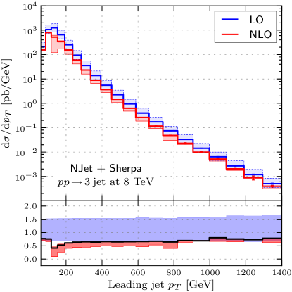
We now present results for three jet production at 8 TeV centre-of-mass energy. Since three jet production has been studied in some detail before [11, 12] we limit our discussion to a few basic quantities. Using the aforementioned setup we find for the total three jet cross section:

$$\sigma_{3}^{\text{8TeV-LO}} =126.65(0.05)^{+66.56}_{-40.40}\>{\rm nb},$$ (18)

$$\sigma_{3}^{\text{8TeV-NLO}} =72.57(0.16)^{+2.71}_{-28.08}\>{\rm nb},$$ (19)

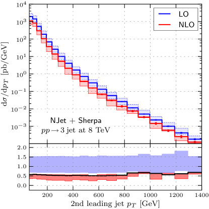
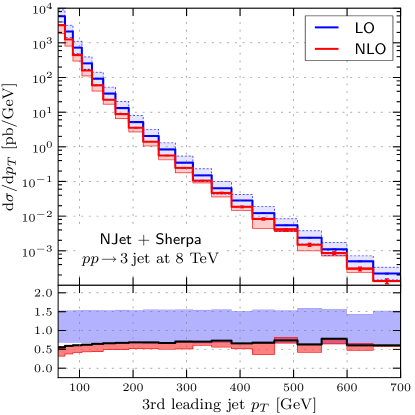
again the numbers in parentheses quote the numerical uncertainty due to the Monte Carlo integration while the sub- and super-scripts show the effect of the scale variation. We note a significant reduction of the scale uncertainty similar to what has been observed for 7 TeV. Furthermore the NLO corrections give a sizeable change of the cross section prediction: The NLO results are reduced by about 40% with respect to the LO cross section again in perfect agreement to what has been observed for 7 TeV in Ref. [60]. Compared to a collider energy of 7 TeV the cross sections are about 35% larger as a consequence of the increased parton fluxes at 8 TeV. As a technical side remark we point out that the numerical integration is very well under control: The numerical uncertainty for the central value amounts to about 2 per mille. In Fig. 1 we show results for the $p_{T}$ distribution of the leading jet. As for the total three jet corrections we observe a sizeable reduction of the NLO prediction with respect to the leading order result. The scale uncertainty is reduced to about 25% of the LO scale uncertainty. With the exception of the low $p_{T}$ region we observe a rather constant K-factor. The dynamical scale chosen for the renormalization and factorization scale indeed avoids large logarithmic corrections at large $p_{T}$. For small $p_{T}$ we expect that soft gluon corrections become important. A reliable prediction in that region would thus require to go beyond a fixed order calculation. We have also studied the $p_{T}$ distribution for the second and the third jet in the $p_{T}$ ordering. The results are very similar to what is shown in Fig. 1. Again we find a rather flat K-factor. The main difference to the $p_{T}$ distribution of the leading jet is that the corrections are slightly larger. The results are shown in the appendix (Fig. 11 and Fig. 12).

Figure 2: Rapidity distribution in $pp\to 3$ jets for the leading jet at the LHC with a centre-of-mass energy of 8 TeV.

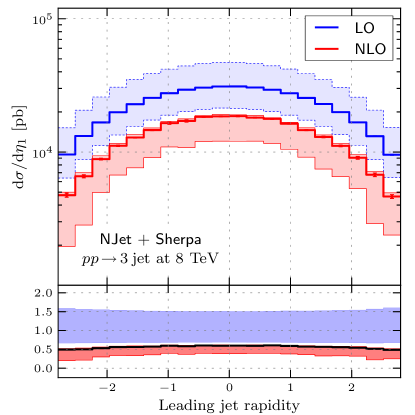
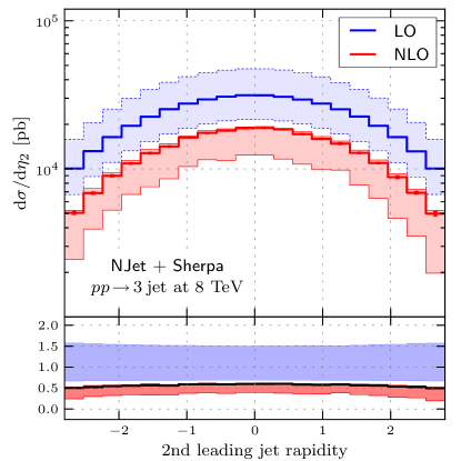
In Fig. 2 we show the rapidity distribution of the leading jet. As in the $p_{T}$ distribution we observe a sizeable correction at NLO together with an important reduction of the scale uncertainty. Again the K-factor is rather flat. We have also analysed the rapidity distribution of the second and third jet. The results look very similar to Fig. 2. The explicit plots are given in the appendix.

3.3 Four Jet Production

In this subsection we present new results for four jet production at NLO accuracy in QCD. Performing a similar analysis as in the three jet case we find for the four jet cross section at 8 TeV:

$$\sigma_{4}^{\text{8TeV-LO}} =14.36(0.01)^{+10.38}_{-5.6}\>{\rm nb},$$ (20)

$$\sigma_{4}^{\text{8TeV-NLO}} =8.15(0.09)^{+0.0}_{-3.24}\>{\rm nb}.$$ (21)

Similar to the findings for 7 TeV the size of the NLO corrections amount to a reduction of $-45$% compared to LO. As far as the scale dependence is concerned a new feature appears compared to the three jet rate: The cross sections for $\mu=\hat{H}_{T}/4$ and $\mu=\hat{H}_{T}$ do not bracket the result for $\mu=\hat{H}_{T}/2$. This is not uncommon for a NLO calculation. While the LO cross section is decreasing as a function of the renormalization scale—a direct consequence of the negative value of the beta function—the NLO scale dependence may develop a plateau showing a flat scale dependence in a restricted region. This is in fact what we would consider as an ideal situation. If the central scale is close to the extrema two additional results obtained by varying the scale by a factor two up and down will be both larger or smaller than the central value. This is precisely what happens in case of the four jet cross section. As central result we quote in Eq. (21) the result for $\mu=\hat{H}_{T}/2$. Assuming that this value is already close to the extrema in the restricted scale range $\hat{H}_{T}/4<\mu<\hat{H}_{T}$ we set the super-script describing the upwards variation to zero. The sub-script describing the downwards variation is obtained from $\min(\sigma_{4}^{\text{8TeV-NLO}}(\mu=\hat{H}_{T}/4),\sigma_{4}^{\rm 8TeV-NLO}(\mu=\hat{H}_{T}))$. Using the explicit results for $\mu=\hat{H}_{T}/4$ and $\mu=\hat{H}_{T}$

$$\sigma_{4}^{\text{8TeV-NLO}}(\mu=\hat{H}_{T}) =7.91(0.05)\>{\rm nb},$$ (22)

$$\sigma_{4}^{\text{8TeV-NLO}}(\mu=\hat{H}_{T}/4) =4.91(0.15)\>{\rm nb},$$ (23)

thus we get the quoted value for the lower scale variation band, $-3.24\>{\rm nb}$. As in the three jet case moving from 7 TeV collider energy to 8 TeV increases the cross section. For the four jet cross section the effect is with about 50% slightly larger than for the three jet rate. We also mentioned that the relative numerical uncertainty due to the Monte Carlo integration is of the order of 1%. The larger uncertainty compared to the three jet cross section reflects the fact that the integration is much more involved. Although not a physical observable it is illustrative to study the contributions from different parton channels. The result is shown in Tab. 2. Note that we do not distinguish between quarks and anti-quarks in the initial state. For example the qq channel includes the contribution from the initial states $q{\overline{q}}^{\prime},qq^{\prime},{\overline{q}}{\overline{q}}^{\prime}$. Furthermore we do not distinguish different quark flavours.

	gg	qg	qq
relative contribution	$37\%$	$49\%$	$14\%$

Table 2: Relative contribution of the different parton channels to $pp\to 4$ jets at LO.

As can be seen the dominant channels are those with one gluon and one quark in the initial state. This is a direct consequence of the sizeable partonic cross section in combination with the largest parton luminosity. $31\%$ of the $49\%$ from these channels come from $gu\to u+3g$ and $gd\to d+3g$. The largest single process is $gg\to 4g$ which contributes $30\%$. As in the three jet case we show in Fig. 3 the $p_{T}$ distribution of the leading jet.

Figure 3: $p_{T}$ distribution in $pp\to 4$ jets for the leading jet at the LHC with a centre-of-mass energy of 8 TeV.

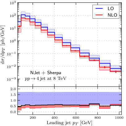
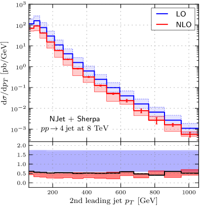
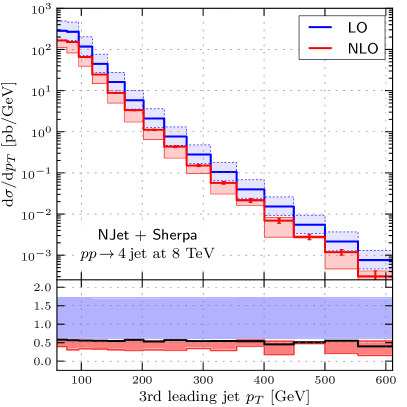
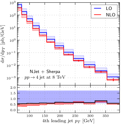
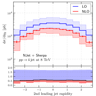
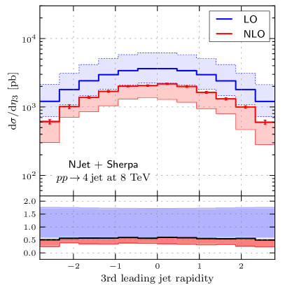
The behaviour follows closely what has been observed in the three jet case. The scale dependence of the NLO result is significantly reduced compared to the LO prediction. Again the K-factor is almost constant over a wide $p_{T}$ range. We find a negative correction of about 45% — in agreement with the findings for the ‘inclusive’ four jet cross section. Only for extreme $p_{T}$ values the K-factor changes significantly. For small $p_{T}$ this might again be a consequence of soft gluon corrections which would require to go beyond fixed order perturbation theory. At large $p_{T}$ the uncertainties due to the numerical integration become important, so that the results become unreliable. The $p_{T}$ distributions of the remaining jets follow pretty much the same pattern. The corresponding K-factor is even more stable compared to the $p_{T}$ distribution of the highest $p_{T}$ jet. The results are shown in Fig. 15, Fig. 16 and Fig. 17 in the appendix. In Fig. 4 the rapidity distribution of the leading jet is shown. The qualitative findings are similar to the $p_{T}$ distribution: Reduction of the NLO cross sections by about 45–50%, significant reduction of the scale dependence and a K-factor which is almost constant over the phase space sampled by the distributions. Looking into the rapidity distributions of the remaining jets we find the same picture.

Figure 4: Rapidity distribution in $pp\to 4$ jets for the leading jet at the LHC with a centre-of-mass energy of 8 TeV.

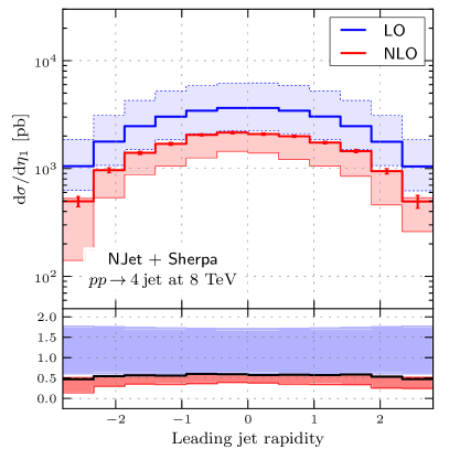
Again we refer to the appendix for the corresponding plots. We notice that the rapidity distributions of the different jets look remarkable similar. To study this in more detail we investigated the ratio

$$R_{j}=\frac{d\sigma_{4}}{d\eta_{j}}\bigg{/}\frac{d\sigma_{4}}{d\eta_{1}}.$$ (24)

The result for $R_{2}$ is shown in Fig. 5.

Figure 5: Ratio $R_{2}$ of the rapidity distribution for the second jet with respect to the leading jet.

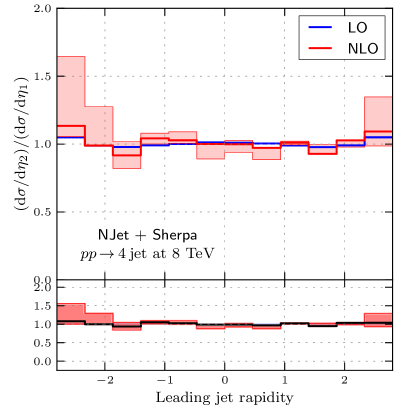
Two important aspects are visible: First of all the ratio is remarkably stable with respect to perturbative corrections. Within the numerical uncertainties LO and NLO results are in perfect agreement. We also show the effects due to scale variation. However since in the ratio the leading power in $\alpha_{s}$ cancels the scale variation is not necessarily a reliable estimate of the theoretical uncertainty. An alternative way to assess the effect of higher order corrections would be to compare the ratio expanded in $\alpha_{s}$ with the naive ratio where we just divide the predictions for the numerator and the denominator. However since we use a dynamical scale setting procedure this is not possible. The second important observation is that to good approximation we have $R_{2}\approx 1$ consistent with the naive expectation. The results for $R_{3}$ and $R_{4}$ look very similar. Experimentally a measurement of the different ratios could be used to validate detector efficiencies and to further constrain the jet energy scale.

The stability of the results shown in Fig. 5 is related to the fact that in the ratio the almost constant K-factor cancels out. In general it might be beneficial to study normalized distributions since in the ratio many uncertainties may cancel. This is evidently true for $\alpha_{s}$ but should also hold to some extent for uncertainties due to the parton distribution functions.

Figure 6: Normalized $p_{T}$ distribution of the leading jet in $pp\to 4$ jets.

Figure 7: Normalized eta distribution of the leading jet in $pp\to 4$ jets.

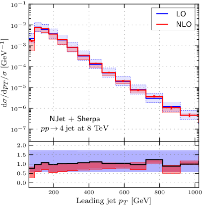
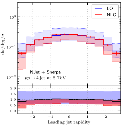
In Fig. 6 and Fig. 7 we show the normalized distributions for the leading jet. Compared to the un-normalized distributions the size of the corrections is reduced. In the rapidity distribution for example the K-factor becomes close to one. Again we stress that the scale uncertainty does not necessarily provide a reliable estimate of theoretical uncertainty. We mentioned in the description of the numerical setup that the LO PDFs come with a rather large value for $\alpha_{s}$. Observing the sizeable NLO corrections — about 40% in case of the three jet cross sections and 45% for the four jet cross section — one may ask how much of the corrections are actually due to the shift in $\alpha_{s}$. Furthermore it would be interesting to disentangle the perturbative corrections of the hard scattering from the change of the PDFs when moving from LO to NLO. To do so we show in Fig. 8 and Fig. 9 results where we have used NLO PDFs together with the respective $\alpha_{s}$ value to evaluate the LO cross sections.

Figure 8: $p_{T}$ distribution of the leading jet in $pp\to 4$ jets using NLO PDFs in the evaluation of the LO cross section.

Figure 9: Normalized eta distribution of the leading jet in $pp\to 4$ jets using NLO PDFs in the evaluation of the LO cross section.

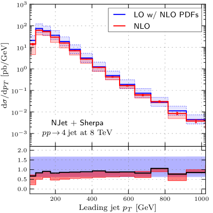
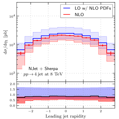
We see that in this way the size of the NLO corrections is roughly divided by two. We also observe that LO and NLO predictions overlap taking the scale uncertainty as an uncertainty estimate of uncalculated higher orders. From a phenomenological point of view we are lead to the conclusion that using the NLO setup in the evaluation of the LO cross sections gives a much better approximation to what happens at NLO accuracy compared to the default setup with LO PDFs. This is a valuable information for the experimental analysis in cases where the NLO corrections are not available or take to long to be evaluated. In general it would be interesting to investigate whether the observations we made here in the case of the four jet cross section hold true for a wider class of NLO processes. It is conceivable that a similar procedure also works for other processes. The reasoning behind the large LO $\alpha_{s}$ value is to account for the NLO corrections to the matrix elements which are not considered in the LO partonic cross sections. However for this to work for a large variety of different processes would require a universal K-factor for NLO corrections. Since K-factors can be rather different for different processes there is an obvious limitation of the procedure. Naively one could expect that this becomes in particular true when cross sections are considered which are of different order in $\alpha_{s}$ compared to the cross sections which enter PDF fits. In such cases using an NLO setting in the evaluation of LO cross sections may provide a better approximation to the ‘full’ (NLO) answer.

3.4 Comparison of three and four jet production

As reference value we have calculated also the two jet cross section using the same setup as before:

$$\sigma_{2}^{\text{8TeV-LO}} =1234.9(1.2)\>{\rm nb},$$ (25)

$$\sigma_{2}^{\text{8TeV-NLO}} =1524.9(2.8)\>{\rm nb}.$$ (26)

Combining (not quite consistent in $\alpha_{s}$ and ignoring soft gluon resummation) the results of Eq. (19), Eq. (21), and Eq. (26) we estimate the total jet cross section to be of the order of 1600 nb. We thus obtain for the 2 : 3 : 4 jet ratios: 1 : 0.05 : 0.005. Only 5% of the multi-jet events are three jet events. The four jet topology is further reduced by a factor 1/10. It is interesting to study how the ratio between four jet production and three jet production behaves as function of the leading jet $p_{T}$. Similar to what has been shown in Ref. [60] we analyse the ratio

$$\frac{d\sigma_{4}}{dp_{T}}\bigg{/}\frac{d\sigma_{3}}{dp_{T}}.$$ (27)

Figure 10: Comparison of three and four jet production.

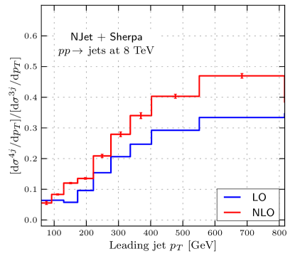
We observe in Fig. 10 that the reduction of the four jet cross section with respect to the three jet cross section is mostly due to the low $p_{T}$ region. At large $p_{T}$ the fraction of four jet events with respect to three jet events raises. In leading order the fraction is about 1/3 at 800 GeV while in NLO it is close to 1/2. With the exception of the low $p_{T}$ region we find that the K-factor is rather constant and takes a value of about 1.4. Note that we have not shown the scale variation in Fig. 10. Since in the ratio the scale dependence would largely cancel the scale dependence will not provide a reliable estimate of the uncalculated higher orders. Note that the results shown here slightly differ from what has been shown in Ref. [60]. We expect the differences to be a consequence of the different bin sizes and the different $R$ value used in the anti-kt jet algorithm.

4 Conclusions

We have presented a study of three and four jet production at the LHC running at a centre-of-mass energy of 8 TeV. The virtual corrections were efficiently evaluated using an on-shell unitarity based method implemented in the publicly available NJet C++ library. We have cross checked the virtual corrections for individual phase space points as far as possible with existing results. We find complete agreement. The complicated structure of real radiation processes was treated within the Catani-Seymour dipole subtraction method. We used the Sherpa Monte Carlo program for this. As an important cross check of our approach we reproduced results for LHC at 7 TeV published recently by the BlackHat collaboration. We find perfect agreement. We stress that this comparison represents the first independent check of the results given in Ref. [60]. The calculation documented in this article nicely illustrates the performance of the NJet library to evaluate QCD one-loop corrections.

For the three and four jet cross sections we find the NLO corrections behave similarly to those obtained at 7 TeV. The NLO corrections reduce the LO cross sections by about 40–50% depending on the jet multiplicity. Compared to the 7 TeV results the cross sections are increased by about 50% due to the larger collider energy and the related increase in the parton fluxes. We have also studied differential distributions. The dynamical scale setting procedure results in an almost constant K-factor leading to very stable results for the normalized distributions. To pin down the origin of the large negative corrections observed in the cross sections and in the unnormalized distributions we have analysed the impact of the LO PDFs used in the LO predictions. Using an NLO setup in the LO calculation shows that the large negative corrections are largely due to the change in the PDFs when going from LO to NLO with the $\alpha_{s}$ value being of particular importance.

The corresponding data for all the plots shown in this article is tabulated in appendix B.

We stress that the results presented here are in fixed order perturbation theory. Large corrections at low $p_{T}$ due to soft gluon emission may require to go beyond fixed order in perturbation theory to achieve a good agreement with the data. Significant progress has been obtained in the matching of NLO calculations with parton shower predictions. For a number of phenomenologically important processes matched results are now available and the automation is pushed forward in two different frameworks ((a)MC@NLO [75, 76, 77] and POWHEG [78, 79]). Studies of di-jet production at NLO with parton showering have recently been performed using both methods [80, 81]. Since the NJet library we developed to perform the calculation presented here is publicly available all required ingredients to include four jet production in (a)MC@NLO or POWHEG are available. We also note that the NJet library includes the virtual corrections required for the calculation of the five jet cross section at NLO accuracy.

Appendix A Additional differential distributions for three and four jet production

In this section we show results for the transverse momentum and rapidity distributions of the subleading jets. Since they show a behaviour rather similar to the leading jet they were not discussed in detail in the main text.

Figure 11: $p_{T}$ distribution in $pp\to 3$ jets for the $2^{\rm nd}$ jet at the LHC with a centre-of-mass energy of 8 TeV.

Figure 12: $p_{T}$ distribution in $pp\to 3$ jets for the $3^{\rm rd}$ jet at the LHC with a centre-of-mass energy of 8 TeV.

Figure 13: Rapidity distribution in $pp\to 3$ jets for the $2^{\rm nd}$ jet at the LHC with a centre-of-mass energy of 8 TeV.

Figure 14: Rapidity distribution in $pp\to 3$ jets for the $3^{\rm rd}$ jet at the LHC with a centre-of-mass energy of 8 TeV.

Figure 15: $p_{T}$ distribution in $pp\to 4$ jets for the $2^{\rm nd}$ jet at the LHC with a centre-of-mass energy of 8 TeV.

Figure 16: $p_{T}$ distribution in $pp\to 4$ jets for the $3^{\rm rd}$ jet at the LHC with a centre-of-mass energy of 8 TeV.

Figure 17: $p_{T}$ distribution in $pp\to 4$ jets for the $4^{\rm th}$ jet at the LHC with a centre-of-mass energy of 8 TeV.

Figure 18: Rapidity distribution in $pp\to 4$ jets for the $2^{\rm nd}$ jet at the LHC with a centre-of-mass energy of 8 TeV.

Figure 19: Rapidity distribution in $pp\to 4$ jets for the $3^{\rm rd}$ jet at the LHC with a centre-of-mass energy of 8 TeV.

Figure 20: Rapidity distribution in $pp\to 4$ jets for the $4^{\rm th}$ jet at the LHC with a centre-of-mass energy of 8 TeV.

Appendix B Tables of differential distributions for three jet production

For future experimental and theoretical studies it might be useful to present the data shown in the figures also in numerical form. In the following we give for all the plots shown in the article the results obtained in the numerical integration.

$p_{T,1}$ (GeV)	LO (pb)	NLO (pb)
$60.0$ — $86.8$	$5606.3$ $(14.6)$	$4316.1$ $(80.8)$
$86.8$ — $117.8$	$32747.4$ $(28.7)$	$24813.3$ $(163.1)$
$117.8$ — $153.1$	$43942.3$ $(34.2)$	$18293.4$ $(219.5)$
$153.1$ — $192.6$	$25597.3$ $(22.2)$	$13464.8$ $(116.1)$
$192.6$ — $236.3$	$11019.8$ $(13.3)$	$6705.3$ $(49.8)$
$236.3$ — $284.3$	$4504.2$ $(6.7)$	$2873.1$ $(21.2)$
$284.3$ — $336.5$	$1854.8$ $(3.6)$	$1208.5$ $(15.8)$
$336.5$ — $392.9$	$779.9$ $(2.1)$	$501.9$ $(5.2)$
$392.9$ — $453.5$	$334.4$ $(1.3)$	$220.6$ $(3.1)$
$453.5$ — $518.4$	$145.8$ $(0.7)$	$94.6$ $(1.5)$
$518.4$ — $587.5$	$65.8$ $(0.5)$	$43.2$ $(0.7)$
$587.5$ — $660.9$	$29.2$ $(0.2)$	$19.3$ $(0.4)$
$660.9$ — $738.5$	$13.5$ $(0.2)$	$9.1$ $(0.3)$
$738.5$ — $820.3$	$6.10$ $(0.09)$	$3.9$ $(0.1)$
$820.3$ — $906.3$	$2.84$ $(0.06)$	$2.0$ $(0.1)$
$906.3$ — $996.6$	$1.29$ $(0.03)$	$0.89$ $(0.06)$
$996.6$ — $1091.1$	$0.60$ $(0.02)$	$0.49$ $(0.03)$
$1091.1$ — $1189.8$	$0.267$ $(0.009)$	$0.20$ $(0.01)$
$1189.8$ — $1292.8$	$0.123$ $(0.005)$	$0.09$ $(0.02)$
$1292.8$ — $1400.0$	$0.054$ $(0.003)$	$0.043$ $(0.004)$

Table 3: Table for the $p_{T}$ distribution of the 1${}^{\text{st}}$ jet in $pp\to 3$ jets.

$p_{T,2}$ (GeV)	LO (pb)	NLO (pb)
$60.0$ — $86.8$	$51490.8$ $(39.9)$	$29576.7$ $(204.4)$
$86.8$ — $117.8$	$43903.6$ $(30.1)$	$25597.6$ $(174.4)$
$117.8$ — $153.1$	$18638.5$ $(17.7)$	$10495.8$ $(97.3)$
$153.1$ — $192.6$	$7441.0$ $(9.4)$	$4129.0$ $(38.7)$
$192.6$ — $236.3$	$2995.0$ $(5.0)$	$1617.8$ $(19.5)$
$236.3$ — $284.3$	$1243.1$ $(3.0)$	$660.4$ $(10.7)$
$284.3$ — $336.5$	$522.6$ $(1.7)$	$276.0$ $(3.6)$
$336.5$ — $392.9$	$229.9$ $(1.2)$	$118.9$ $(2.2)$
$392.9$ — $453.5$	$101.6$ $(0.7)$	$54.2$ $(1.2)$
$453.5$ — $518.4$	$46.3$ $(0.4)$	$24.1$ $(0.7)$
$518.4$ — $587.5$	$21.4$ $(0.2)$	$10.9$ $(0.4)$
$587.5$ — $660.9$	$9.7$ $(0.2)$	$4.9$ $(0.3)$
$660.9$ — $738.5$	$4.46$ $(0.09)$	$2.3$ $(0.1)$
$738.5$ — $820.3$	$2.13$ $(0.06)$	$1.2$ $(0.1)$
$820.3$ — $906.3$	$0.98$ $(0.04)$	$0.65$ $(0.07)$
$906.3$ — $996.6$	$0.45$ $(0.02)$	$0.30$ $(0.03)$
$996.6$ — $1091.1$	$0.22$ $(0.01)$	$0.14$ $(0.02)$
$1091.1$ — $1189.8$	$0.099$ $(0.006)$	$0.056$ $(0.007)$
$1189.8$ — $1292.8$	$0.043$ $(0.003)$	$0.027$ $(0.004)$
$1292.8$ — $1400.0$	$0.020$ $(0.001)$	$0.013$ $(0.002)$

Table 4: Table for the $p_{T}$ distribution of the 2${}^{\text{nd}}$ jet in $pp\to 3$ jets.

$p_{T,3}$ (GeV)	LO (pb)	NLO (pb)
$60.0$ — $72.8$	$74805.4$ $(46.5)$	$41272.9$ $(208.2)$
$72.8$ — $87.6$	$31467.0$ $(23.7)$	$18659.0$ $(90.8)$
$87.6$ — $104.5$	$12270.2$ $(12.5)$	$7475.7$ $(50.6)$
$104.5$ — $123.3$	$4819.1$ $(6.4)$	$3008.2$ $(23.0)$
$123.3$ — $144.2$	$1928.3$ $(3.6)$	$1244.0$ $(14.5)$
$144.2$ — $167.1$	$789.0$ $(1.9)$	$523.2$ $(6.7)$
$167.1$ — $192.0$	$326.9$ $(1.1)$	$219.4$ $(2.7)$
$192.0$ — $219.0$	$139.4$ $(0.6)$	$95.4$ $(2.8)$
$219.0$ — $248.0$	$59.4$ $(0.3)$	$40.6$ $(0.8)$
$248.0$ — $278.9$	$26.0$ $(0.2)$	$17.4$ $(0.7)$
$278.9$ — $312.0$	$11.48$ $(0.09)$	$8.1$ $(0.2)$
$312.0$ — $347.0$	$5.25$ $(0.06)$	$3.7$ $(0.1)$
$347.0$ — $384.0$	$2.37$ $(0.03)$	$1.73$ $(0.09)$
$384.0$ — $423.1$	$1.10$ $(0.02)$	$0.72$ $(0.04)$
$423.1$ — $464.2$	$0.503$ $(0.010)$	$0.34$ $(0.03)$
$464.2$ — $507.3$	$0.235$ $(0.005)$	$0.17$ $(0.01)$
$507.3$ — $552.5$	$0.107$ $(0.003)$	$0.067$ $(0.007)$
$552.5$ — $599.6$	$0.052$ $(0.002)$	$0.041$ $(0.004)$
$599.6$ — $648.8$	$0.0244$ $(0.0009)$	$0.015$ $(0.002)$
$648.8$ — $700.0$	$0.0113$ $(0.0005)$	$0.007$ $(0.001)$

Table 5: Table for the $p_{T}$ distribution of the 3${}^{\text{rd}}$ jet in $pp\to 3$ jets.

$\eta_{1}$	LO (pb)	NLO (pb)
$-2.8$ — $(-2.5)$	$2683.1$ $(16.1)$	$1328.9$ $(46.8)$
$-2.5$ — $(-2.2)$	$3692.9$ $(15.3)$	$1842.1$ $(47.8)$
$-2.2$ — $(-2.0)$	$4669.0$ $(12.9)$	$2477.9$ $(37.6)$
$-2.0$ — $(-1.7)$	$5567.8$ $(12.0)$	$3122.1$ $(36.3)$
$-1.7$ — $(-1.4)$	$6398.3$ $(11.2)$	$3597.6$ $(34.4)$
$-1.4$ — $(-1.1)$	$7139.7$ $(10.4)$	$4093.4$ $(37.6)$
$-1.1$ — $(-0.8)$	$7739.4$ $(10.1)$	$4613.4$ $(90.7)$
$-0.8$ — $(-0.6)$	$8220.6$ $(10.0)$	$4790.3$ $(95.9)$
$-0.6$ — $(-0.3)$	$8518.6$ $(9.5)$	$5139.7$ $(37.9)$
$-0.3$ — $(0.0)$	$8683.8$ $(9.5)$	$5184.0$ $(40.4)$
$0.0$ — $0.3$	$8696.8$ $(9.6)$	$5208.2$ $(51.7)$
$0.3$ — $0.6$	$8541.3$ $(9.5)$	$5073.1$ $(42.3)$
$0.6$ — $0.8$	$8208.1$ $(9.7)$	$4967.0$ $(37.2)$
$0.8$ — $1.1$	$7730.9$ $(10.1)$	$4571.0$ $(34.3)$
$1.1$ — $1.4$	$7129.7$ $(10.6)$	$4090.0$ $(34.6)$
$1.4$ — $1.7$	$6421.9$ $(11.3)$	$3632.4$ $(44.6)$
$1.7$ — $2.0$	$5580.1$ $(12.1)$	$3113.5$ $(45.6)$
$2.0$ — $2.2$	$4677.1$ $(13.7)$	$2536.4$ $(60.3)$
$2.2$ — $2.5$	$3682.1$ $(14.8)$	$1890.8$ $(59.3)$
$2.5$ — $2.8$	$2670.7$ $(18.5)$	$1299.0$ $(42.9)$

Table 6: Table for the rapidity distribution of the 1${}^{\text{st}}$ jet in $pp\to 3$ jets.

$\eta_{2}$	LO (pb)	NLO (pb)
$-2.8$ — $(-2.5)$	$2815.4$ $(13.9)$	$1413.7$ $(36.2)$
$-2.5$ — $(-2.2)$	$3688.7$ $(12.9)$	$1921.8$ $(35.9)$
$-2.2$ — $(-2.0)$	$4591.1$ $(11.6)$	$2511.6$ $(45.0)$
$-2.0$ — $(-1.7)$	$5473.5$ $(11.7)$	$3047.2$ $(39.3)$
$-1.7$ — $(-1.4)$	$6304.7$ $(11.7)$	$3578.4$ $(48.0)$
$-1.4$ — $(-1.1)$	$7083.9$ $(11.9)$	$3967.2$ $(47.7)$
$-1.1$ — $(-0.8)$	$7727.6$ $(11.1)$	$4556.2$ $(41.9)$
$-0.8$ — $(-0.6)$	$8250.3$ $(11.8)$	$4901.3$ $(46.6)$
$-0.6$ — $(-0.3)$	$8609.4$ $(11.5)$	$5078.2$ $(45.0)$
$-0.3$ — $(0.0)$	$8803.3$ $(11.6)$	$5269.1$ $(59.3)$
$0.0$ — $0.3$	$8788.3$ $(11.3)$	$5284.6$ $(46.5)$
$0.3$ — $0.6$	$8596.2$ $(11.6)$	$5176.7$ $(51.4)$
$0.6$ — $0.8$	$8234.9$ $(11.8)$	$4807.0$ $(48.9)$
$0.8$ — $1.1$	$7732.1$ $(11.5)$	$4462.6$ $(45.6)$
$1.1$ — $1.4$	$7080.3$ $(12.9)$	$4145.7$ $(66.0)$
$1.4$ — $1.7$	$6319.7$ $(12.1)$	$3591.5$ $(43.4)$
$1.7$ — $2.0$	$5468.7$ $(12.0)$	$3067.9$ $(37.7)$
$2.0$ — $2.2$	$4588.0$ $(12.5)$	$2462.2$ $(51.4)$
$2.2$ — $2.5$	$3680.5$ $(12.7)$	$1931.2$ $(40.3)$
$2.5$ — $2.8$	$2815.3$ $(13.7)$	$1396.6$ $(46.7)$

Table 7: Table for the rapidity distribution of the 2${}^{\text{nd}}$ jet in $pp\to 3$ jets.

$\eta_{3}$	LO (pb)	NLO (pb)
$-2.8$ — $(-2.5)$	$3102.7$ $(12.3)$	$1558.4$ $(46.9)$
$-2.5$ — $(-2.2)$	$3877.2$ $(13.3)$	$2069.5$ $(43.4)$
$-2.2$ — $(-2.0)$	$4704.9$ $(11.2)$	$2524.2$ $(45.5)$
$-2.0$ — $(-1.7)$	$5507.7$ $(11.5)$	$3091.2$ $(43.8)$
$-1.7$ — $(-1.4)$	$6294.6$ $(12.4)$	$3660.3$ $(47.9)$
$-1.4$ — $(-1.1)$	$7005.9$ $(11.4)$	$4030.4$ $(42.4)$
$-1.1$ — $(-0.8)$	$7628.2$ $(11.7)$	$4385.8$ $(51.1)$
$-0.8$ — $(-0.6)$	$8117.4$ $(12.0)$	$4766.5$ $(40.8)$
$-0.6$ — $(-0.3)$	$8464.6$ $(12.2)$	$5028.8$ $(42.0)$
$-0.3$ — $(0.0)$	$8649.2$ $(12.9)$	$5012.9$ $(50.5)$
$0.0$ — $0.3$	$8652.7$ $(12.5)$	$5081.1$ $(47.0)$
$0.3$ — $0.6$	$8467.3$ $(12.3)$	$4897.5$ $(54.5)$
$0.6$ — $0.8$	$8109.7$ $(12.0)$	$4927.0$ $(51.2)$
$0.8$ — $1.1$	$7626.6$ $(12.5)$	$4463.0$ $(51.9)$
$1.1$ — $1.4$	$7005.6$ $(12.5)$	$4112.4$ $(68.9)$
$1.4$ — $1.7$	$6272.6$ $(11.4)$	$3639.6$ $(40.9)$
$1.7$ — $2.0$	$5487.1$ $(11.3)$	$3050.4$ $(43.4)$
$2.0$ — $2.2$	$4717.6$ $(12.3)$	$2577.2$ $(55.2)$
$2.2$ — $2.5$	$3872.4$ $(12.1)$	$2090.8$ $(34.1)$
$2.5$ — $2.8$	$3087.8$ $(12.4)$	$1603.9$ $(37.7)$

Table 8: Table for the rapidity distribution of the 3${}^{\text{rd}}$ jet in $pp\to 3$ jets.

Appendix C Tables of differential distributions for four jet production

$p_{T,1}$ (GeV)	LO (pb)	NLO (pb)
$60.0$ — $92.0$	$1013.0$ $(3.8)$	$446.9$ $(41.5)$
$92.0$ — $129.6$	$4204.4$ $(3.3)$	$2335.6$ $(57.6)$
$129.6$ — $172.9$	$3775.5$ $(2.4)$	$2303.3$ $(43.1)$
$172.9$ — $221.9$	$2626.8$ $(1.9)$	$1452.7$ $(31.5)$
$221.9$ — $276.5$	$1498.8$ $(1.4)$	$867.7$ $(22.6)$
$276.5$ — $336.7$	$707.1$ $(0.8)$	$417.7$ $(11.1)$
$336.7$ — $402.6$	$308.8$ $(0.4)$	$187.0$ $(5.1)$
$402.6$ — $474.1$	$131.5$ $(0.3)$	$83.2$ $(3.1)$
$474.1$ — $551.3$	$55.4$ $(0.1)$	$32.5$ $(1.6)$
$551.3$ — $634.1$	$23.32$ $(0.08)$	$13.8$ $(0.9)$
$634.1$ — $722.6$	$9.79$ $(0.05)$	$5.4$ $(0.5)$
$722.6$ — $816.7$	$4.09$ $(0.03)$	$2.9$ $(0.2)$
$816.7$ — $916.5$	$1.69$ $(0.02)$	$0.9$ $(0.1)$
$916.5$ — $1021.9$	$0.705$ $(0.009)$	$0.40$ $(0.07)$

Table 9: Table for the $p_{T}$ distribution of the 1${}^{\text{st}}$ jet in $pp\to 4$ jets.

$p_{T,2}$ (GeV)	LO (pb)	NLO (pb)
$60.0$ — $89.8$	$3412.4$ $(4.8)$	$2088.7$ $(58.8)$
$89.8$ — $124.8$	$5607.7$ $(3.1)$	$3173.1$ $(56.4)$
$124.8$ — $165.1$	$3031.8$ $(1.9)$	$1670.4$ $(34.1)$
$165.1$ — $210.6$	$1342.6$ $(1.1)$	$700.9$ $(16.3)$
$210.6$ — $261.4$	$563.4$ $(0.7)$	$304.7$ $(8.5)$
$261.4$ — $317.5$	$233.4$ $(0.4)$	$125.9$ $(4.3)$
$317.5$ — $378.8$	$97.5$ $(0.2)$	$49.1$ $(2.3)$
$378.8$ — $445.4$	$41.5$ $(0.1)$	$21.5$ $(1.4)$
$445.4$ — $517.2$	$17.77$ $(0.08)$	$9.0$ $(0.7)$
$517.2$ — $594.2$	$7.59$ $(0.05)$	$3.9$ $(0.3)$
$594.2$ — $676.6$	$3.27$ $(0.03)$	$1.9$ $(0.3)$
$676.6$ — $764.2$	$1.42$ $(0.02)$	$0.7$ $(0.1)$
$764.2$ — $857.0$	$0.61$ $(0.01)$	$0.25$ $(0.09)$
$857.0$ — $955.1$	$0.264$ $(0.006)$	$0.16$ $(0.03)$
$955.1$ — $1058.4$	$0.113$ $(0.004)$	$0.06$ $(0.02)$

Table 10: Table for the $p_{T}$ distribution of the 2${}^{\text{nd}}$ jet in $pp\to 4$ jets.

$p_{T,3}$ (GeV)	LO (pb)	NLO (pb)
$60.0$ — $76.4$	$4670.9$ $(5.1)$	$2710.4$ $(70.8)$
$76.4$ — $95.8$	$5196.7$ $(3.0)$	$2941.8$ $(48.8)$
$95.8$ — $118.0$	$2617.1$ $(1.7)$	$1463.5$ $(25.4)$
$118.0$ — $143.2$	$1123.2$ $(0.9)$	$619.2$ $(13.2)$
$143.2$ — $171.2$	$455.2$ $(0.5)$	$247.8$ $(6.7)$
$171.2$ — $202.2$	$180.5$ $(0.3)$	$103.7$ $(3.0)$
$202.2$ — $236.1$	$71.1$ $(0.1)$	$37.9$ $(1.6)$
$236.1$ — $272.8$	$28.10$ $(0.08)$	$15.9$ $(0.8)$
$272.8$ — $312.5$	$11.08$ $(0.04)$	$6.0$ $(0.4)$
$312.5$ — $355.0$	$4.46$ $(0.02)$	$2.4$ $(0.2)$
$355.0$ — $400.5$	$1.80$ $(0.01)$	$1.0$ $(0.1)$
$400.5$ — $448.9$	$0.737$ $(0.008)$	$0.33$ $(0.05)$
$448.9$ — $500.1$	$0.281$ $(0.004)$	$0.14$ $(0.02)$
$500.1$ — $554.3$	$0.116$ $(0.002)$	$0.064$ $(0.010)$
$554.3$ — $611.4$	$0.0434$ $(0.0008)$	$0.017$ $(0.007)$

Table 11: Table for the $p_{T}$ distribution of the 3${}^{\text{rd}}$ jet in $pp\to 4$ jets.

$p_{T,4}$ (GeV)	LO (pb)	NLO (pb)
$60.0$ — $74.2$	$9745.6$ $(5.8)$	$5473.4$ $(80.4)$
$74.2$ — $91.0$	$3178.9$ $(2.0)$	$1811.3$ $(29.9)$
$91.0$ — $110.2$	$984.5$ $(0.8)$	$591.7$ $(13.6)$
$110.2$ — $131.9$	$307.7$ $(0.4)$	$182.8$ $(5.2)$
$131.9$ — $156.2$	$97.5$ $(0.2)$	$61.2$ $(2.0)$
$156.2$ — $183.0$	$31.49$ $(0.07)$	$19.1$ $(0.9)$
$183.0$ — $212.3$	$10.36$ $(0.03)$	$7.2$ $(0.4)$
$212.3$ — $244.1$	$3.45$ $(0.02)$	$2.3$ $(0.2)$
$244.1$ — $278.4$	$1.173$ $(0.008)$	$0.79$ $(0.09)$
$278.4$ — $315.2$	$0.408$ $(0.004)$	$0.27$ $(0.03)$
$315.2$ — $354.5$	$0.142$ $(0.002)$	$0.12$ $(0.02)$
$354.5$ — $396.3$	$0.0491$ $(0.0008)$	$0.030$ $(0.006)$

Table 12: Table for the $p_{T}$ distribution of the 4${}^{\text{th}}$ jet in $pp\to 4$ jets.

$\eta_{1}$	LO (pb)	NLO (pb)
$-2.8$ — $(-2.3)$	$490.6$ $(1.7)$	$231.7$ $(25.6)$
$-2.3$ — $(-1.9)$	$828.3$ $(1.8)$	$450.5$ $(24.8)$
$-1.9$ — $(-1.4)$	$1151.0$ $(1.6)$	$651.9$ $(22.7)$
$-1.4$ — $(-0.9)$	$1413.3$ $(1.8)$	$790.3$ $(24.8)$
$-0.9$ — $(-0.5)$	$1600.9$ $(1.7)$	$957.7$ $(21.9)$
$-0.5$ — $(0.0)$	$1698.2$ $(2.2)$	$1005.6$ $(26.6)$
$0.0$ — $0.5$	$1698.8$ $(2.3)$	$973.1$ $(27.1)$
$0.5$ — $0.9$	$1600.4$ $(1.6)$	$929.5$ $(23.6)$
$0.9$ — $1.4$	$1413.9$ $(1.7)$	$811.2$ $(23.6)$
$1.4$ — $1.9$	$1152.2$ $(1.6)$	$677.0$ $(24.1)$
$1.9$ — $2.3$	$826.0$ $(1.6)$	$440.7$ $(25.1)$
$2.3$ — $2.8$	$487.9$ $(1.6)$	$231.2$ $(32.0)$

Table 13: Table for the rapidity distribution of the 1${}^{\text{st}}$ jet in $pp\to 4$ jets.

$\eta_{2}$	LO (pb)	NLO (pb)
$-2.8$ — $(-2.3)$	$514.8$ $(1.8)$	$262.8$ $(23.9)$
$-2.3$ — $(-1.9)$	$819.3$ $(1.4)$	$445.6$ $(29.8)$
$-1.9$ — $(-1.4)$	$1126.2$ $(1.6)$	$598.0$ $(27.7)$
$-1.4$ — $(-0.9)$	$1399.4$ $(1.7)$	$823.5$ $(23.4)$
$-0.9$ — $(-0.5)$	$1602.2$ $(1.6)$	$984.4$ $(27.8)$
$-0.5$ — $(0.0)$	$1720.2$ $(2.3)$	$1006.7$ $(23.8)$
$0.0$ — $0.5$	$1716.3$ $(2.5)$	$972.4$ $(24.2)$
$0.5$ — $0.9$	$1607.2$ $(1.9)$	$903.8$ $(25.9)$
$0.9$ — $1.4$	$1398.9$ $(1.8)$	$819.4$ $(26.7)$
$1.4$ — $1.9$	$1126.3$ $(1.6)$	$628.3$ $(26.2)$
$1.9$ — $2.3$	$818.3$ $(1.5)$	$452.8$ $(22.6)$
$2.3$ — $2.8$	$512.3$ $(1.4)$	$252.7$ $(23.4)$

Table 14: Table for the rapidity distribution of the 2${}^{\text{nd}}$ jet in $pp\to 4$ jets.

$\eta_{3}$	LO (pb)	NLO (pb)
$-2.8$ — $(-2.3)$	$563.2$ $(1.3)$	$284.2$ $(21.8)$
$-2.3$ — $(-1.9)$	$838.6$ $(1.7)$	$472.9$ $(32.7)$
$-1.9$ — $(-1.4)$	$1124.0$ $(1.5)$	$644.1$ $(21.9)$
$-1.4$ — $(-0.9)$	$1381.6$ $(1.7)$	$787.9$ $(27.2)$
$-0.9$ — $(-0.5)$	$1582.7$ $(2.3)$	$938.1$ $(24.7)$
$-0.5$ — $(0.0)$	$1693.3$ $(2.7)$	$957.9$ $(26.6)$
$0.0$ — $0.5$	$1692.3$ $(1.9)$	$1016.1$ $(27.5)$
$0.5$ — $0.9$	$1580.8$ $(1.8)$	$928.6$ $(27.0)$
$0.9$ — $1.4$	$1382.8$ $(1.7)$	$762.1$ $(27.4)$
$1.4$ — $1.9$	$1122.6$ $(1.6)$	$613.0$ $(25.0)$
$1.9$ — $2.3$	$838.3$ $(1.3)$	$466.2$ $(19.5)$
$2.3$ — $2.8$	$561.3$ $(1.3)$	$279.2$ $(20.4)$

Table 15: Table for the rapidity distribution of the 3${}^{\text{rd}}$ jet in $pp\to 4$ jets.

$\eta_{4}$	LO (pb)	NLO (pb)
$-2.8$ — $(-2.3)$	$572.1$ $(1.5)$	$277.2$ $(17.0)$
$-2.3$ — $(-1.9)$	$834.6$ $(1.4)$	$451.9$ $(28.7)$
$-1.9$ — $(-1.4)$	$1118.4$ $(1.5)$	$652.6$ $(34.0)$
$-1.4$ — $(-0.9)$	$1376.9$ $(1.7)$	$803.5$ $(34.9)$
$-0.9$ — $(-0.5)$	$1579.3$ $(2.0)$	$917.5$ $(25.5)$
$-0.5$ — $(0.0)$	$1695.5$ $(2.5)$	$989.0$ $(27.9)$
$0.0$ — $0.5$	$1695.1$ $(2.0)$	$1002.0$ $(30.4)$
$0.5$ — $0.9$	$1585.7$ $(2.4)$	$916.9$ $(28.1)$
$0.9$ — $1.4$	$1379.1$ $(1.8)$	$789.6$ $(26.3)$
$1.4$ — $1.9$	$1115.4$ $(1.5)$	$638.2$ $(24.8)$
$1.9$ — $2.3$	$837.7$ $(1.5)$	$428.9$ $(20.0)$
$2.3$ — $2.8$	$571.7$ $(1.1)$	$283.1$ $(18.9)$

Table 16: Table for the rapidity distribution of the 4${}^{\text{th}}$ jet in $pp\to 4$ jets.

References

- Badger et al. [2012] S. Badger, B. Biedermann, P. Uwer, V. Yundin, Numerical evaluation of NLO corrections to multi-jet production in massless QCD (2012).
- Mangano et al. [2003] M. L. Mangano, M. Moretti, F. Piccinini, R. Pittau, A. D. Polosa, ALPGEN, a generator for hard multiparton processes in hadronic collisions, JHEP 0307 (2003) 001.
- Gleisberg et al. [2009] T. Gleisberg, S. Hoeche, F. Krauss, M. Schonherr, S. Schumann, et al., Event generation with SHERPA 1.1, JHEP 0902 (2009) 007.
- Gleisberg and Hoeche [2008] T. Gleisberg, S. Hoeche, Comix, a new matrix element generator, JHEP 0812 (2008) 039.
- Alwall et al. [2007] J. Alwall, P. Demin, S. de Visscher, R. Frederix, M. Herquet, et al., MadGraph/MadEvent v4: The New Web Generation, JHEP 0709 (2007) 028.
- Maltoni and Stelzer [2003] F. Maltoni, T. Stelzer, MadEvent: Automatic event generation with MadGraph, JHEP 0302 (2003) 027.
- Alwall et al. [2011] J. Alwall, M. Herquet, F. Maltoni, O. Mattelaer, T. Stelzer, MadGraph 5 : Going Beyond, JHEP 1106 (2011) 128.
- Cafarella et al. [2009] A. Cafarella, C. G. Papadopoulos, M. Worek, Helac-Phegas: A Generator for all parton level processes, Comput.Phys.Commun. 180 (2009) 1941–1955.
- Ellis et al. [1992] S. D. Ellis, Z. Kunszt, D. E. Soper, Two jet production in hadron collisions at order alpha-s**3 in QCD, Phys.Rev.Lett. 69 (1992) 1496–1499.
- Giele et al. [1993] W. Giele, E. N. Glover, D. A. Kosower, Higher order corrections to jet cross-sections in hadron colliders, Nucl.Phys. B403 (1993) 633–670.
- Nagy [2002] Z. Nagy, Three jet cross-sections in hadron hadron collisions at next-to-leading order, Phys.Rev.Lett. 88 (2002) 122003.
- Nagy [2003] Z. Nagy, Next-to-leading order calculation of three jet observables in hadron hadron collision, Phys.Rev. D68 (2003) 094002.
- Kilgore and Giele [1997] W. B. Kilgore, W. Giele, Next-to-leading order gluonic three jet production at hadron colliders, Phys.Rev. D55 (1997) 7183–7190.
- Trocsanyi [1996] Z. Trocsanyi, Three jet cross-section in hadron collisions at next-to-leading order: Pure gluon processes, Phys.Rev.Lett. 77 (1996) 2182–2185.
- Catani and Seymour [1996] S. Catani, M. Seymour, The Dipole formalism for the calculation of QCD jet cross-sections at next-to-leading order, Phys.Lett. B378 (1996) 287–301.
- Gleisberg and Krauss [2008] T. Gleisberg, F. Krauss, Automating dipole subtraction for QCD NLO calculations, Eur.Phys.J. C53 (2008) 501–523.
- Seymour and Tevlin [2008] M. H. Seymour, C. Tevlin, TeVJet: A General framework for the calculation of jet observables in NLO QCD (2008).
- Frederix et al. [2008] R. Frederix, T. Gehrmann, N. Greiner, Automation of the Dipole Subtraction Method in MadGraph/MadEvent, JHEP 0809 (2008) 122.
- Hasegawa et al. [2010] K. Hasegawa, S. Moch, P. Uwer, AutoDipole: Automated generation of dipole subtraction terms, Comput.Phys.Commun. 181 (2010) 1802–1817.
- Czakon et al. [2009] M. Czakon, C. Papadopoulos, M. Worek, Polarizing the Dipoles, JHEP 0908 (2009) 085.
- Frederix et al. [2009] R. Frederix, S. Frixione, F. Maltoni, T. Stelzer, Automation of next-to-leading order computations in QCD: The FKS subtraction, JHEP 0910 (2009) 003.
- Bern et al. [1994] Z. Bern, L. J. Dixon, D. C. Dunbar, D. A. Kosower, One loop n point gauge theory amplitudes, unitarity and collinear limits, Nucl.Phys. B425 (1994) 217–260.
- Bern et al. [1995] Z. Bern, L. J. Dixon, D. C. Dunbar, D. A. Kosower, Fusing gauge theory tree amplitudes into loop amplitudes, Nucl.Phys. B435 (1995) 59–101.
- Berger et al. [2008] C. Berger, Z. Bern, L. Dixon, F. Febres Cordero, D. Forde, et al., An Automated Implementation of On-Shell Methods for One-Loop Amplitudes, Phys.Rev. D78 (2008) 036003.
- Britto et al. [2005] R. Britto, F. Cachazo, B. Feng, Generalized unitarity and one-loop amplitudes in N=4 super-Yang-Mills, Nucl.Phys. B725 (2005) 275–305.
- Forde [2007] D. Forde, Direct extraction of one-loop integral coefficients, Phys.Rev. D75 (2007) 125019.
- Ellis et al. [2008] R. Ellis, W. Giele, Z. Kunszt, A Numerical Unitarity Formalism for Evaluating One-Loop Amplitudes, JHEP 0803 (2008) 003.
- Giele et al. [2008] W. T. Giele, Z. Kunszt, K. Melnikov, Full one-loop amplitudes from tree amplitudes, JHEP 0804 (2008) 049.
- Badger [2009] S. Badger, Direct Extraction Of One Loop Rational Terms, JHEP 0901 (2009) 049.
- Cascioli et al. [2012] F. Cascioli, P. Maierhofer, S. Pozzorini, Scattering Amplitudes with Open Loops, Phys.Rev.Lett. 108 (2012) 111601.
- Becker et al. [2012] S. Becker, D. Goetz, C. Reuschle, C. Schwan, S. Weinzierl, NLO results for five, six and seven jets in electron-positron annihilation, Phys.Rev.Lett. 108 (2012) 032005.
- Berger et al. [2009a] C. Berger, Z. Bern, L. J. Dixon, F. Febres Cordero, D. Forde, et al., Precise Predictions for + 3 Jet Production at Hadron Colliders, Phys.Rev.Lett. 102 (2009a) 222001.
- Berger et al. [2009b] C. Berger, Z. Bern, L. J. Dixon, F. Febres Cordero, D. Forde, et al., Next-to-Leading Order QCD Predictions for W+3-Jet Distributions at Hadron Colliders, Phys.Rev. D80 (2009b) 074036.
- Berger et al. [2010] C. Berger, Z. Bern, L. J. Dixon, F. Febres Cordero, D. Forde, et al., Next-to-Leading Order QCD Predictions for +3-Jet Distributions at the Tevatron, Phys.Rev. D82 (2010) 074002.
- Bredenstein et al. [2009] A. Bredenstein, A. Denner, S. Dittmaier, S. Pozzorini, NLO QCD corrections to pp t anti-t b anti-b + X at the LHC, Phys.Rev.Lett. 103 (2009) 012002.
- Bredenstein et al. [2010] A. Bredenstein, A. Denner, S. Dittmaier, S. Pozzorini, NLO QCD Corrections to Top Anti-Top Bottom Anti-Bottom Production at the LHC: 2. full hadronic results, JHEP 1003 (2010) 021.
- Bevilacqua et al. [2009] G. Bevilacqua, M. Czakon, C. Papadopoulos, R. Pittau, M. Worek, Assault on the NLO Wishlist: t anti-t b anti-b, JHEP 0909 (2009) 109.
- Bevilacqua et al. [2010] G. Bevilacqua, M. Czakon, C. Papadopoulos, M. Worek, Dominant QCD Backgrounds in Higgs Boson Analyses at the LHC: A Study of pp t anti-t + 2 jets at Next-To-Leading Order, Phys.Rev.Lett. 104 (2010) 162002.
- Denner et al. [2011] A. Denner, S. Dittmaier, S. Kallweit, S. Pozzorini, NLO QCD corrections to WWbb production at hadron colliders, Phys.Rev.Lett. 106 (2011) 052001.
- Bevilacqua et al. [2011a] G. Bevilacqua, M. Czakon, A. van Hameren, C. G. Papadopoulos, M. Worek, Complete off-shell effects in top quark pair hadroproduction with leptonic decay at next-to-leading order, JHEP 1102 (2011a) 083.
- Bevilacqua et al. [2011b] G. Bevilacqua, M. Czakon, C. Papadopoulos, M. Worek, Hadronic top-quark pair production in association with two jets at Next-to-Leading Order QCD, Phys.Rev. D84 (2011b) 114017.
- Denner et al. [2012] A. Denner, S. Dittmaier, S. Kallweit, S. Pozzorini, NLO QCD corrections to off-shell top-antitop production with leptonic decays at hadron colliders (2012).
- Bevilacqua and Worek [2012] G. Bevilacqua, M. Worek, Constraining BSM Physics at the LHC: Four top final states with NLO accuracy in perturbative QCD, JHEP 1207 (2012) 111.
- Binoth et al. [2010] T. Binoth, N. Greiner, A. Guffanti, J. Reuter, J.-P. Guillet, et al., Next-to-leading order QCD corrections to pp b anti-b b anti-b + X at the LHC: the quark induced case, Phys.Lett. B685 (2010) 293–296.
- Greiner et al. [2011] N. Greiner, A. Guffanti, T. Reiter, J. Reuter, NLO QCD corrections to the production of two bottom-antibottom pairs at the LHC, Phys.Rev.Lett. 107 (2011) 102002.
- Greiner et al. [2012] N. Greiner, G. Heinrich, P. Mastrolia, G. Ossola, T. Reiter, et al., NLO QCD corrections to the production of W+ W- plus two jets at the LHC, Phys.Lett. B713 (2012) 277–283.
- Melnikov and Zanderighi [2010] K. Melnikov, G. Zanderighi, W+3 jet production at the LHC as a signal or background, Phys.Rev. D81 (2010) 074025.
- Ellis et al. [2009] R. K. Ellis, K. Melnikov, G. Zanderighi, W+3 jet production at the Tevatron, Phys.Rev. D80 (2009) 094002.
- Melia et al. [2011] T. Melia, K. Melnikov, R. Rontsch, G. Zanderighi, NLO QCD corrections for pair production in association with two jets at hadron colliders, Phys.Rev. D83 (2011) 114043.
- Melia et al. [2010] T. Melia, K. Melnikov, R. Rontsch, G. Zanderighi, Next-to-leading order QCD predictions for production at the LHC, JHEP 1012 (2010) 053.
- Campanario [2011] F. Campanario, Towards at NLO QCD: Bosonic contributions to triple vector boson production plus jet, JHEP 1110 (2011) 070.
- Campanario et al. [2011] F. Campanario, C. Englert, M. Rauch, D. Zeppenfeld, Precise predictions for W +jet production at hadron colliders, Phys.Lett. B704 (2011) 515–519.
- Berger et al. [2011] C. Berger, Z. Bern, L. J. Dixon, F. Febres Cordero, D. Forde, et al., Precise Predictions for W + 4 Jet Production at the Large Hadron Collider, Phys.Rev.Lett. 106 (2011) 092001.
- Ita et al. [2012] H. Ita, Z. Bern, L. Dixon, F. Febres Cordero, D. Kosower, et al., Precise Predictions for Z + 4 Jets at Hadron Colliders, Phys.Rev. D85 (2012) 031501.
- Frederix et al. [2010] R. Frederix, S. Frixione, K. Melnikov, G. Zanderighi, NLO QCD corrections to five-jet production at LEP and the extraction of , JHEP 1011 (2010) 050.
- Badger et al. [2011] S. Badger, B. Biedermann, P. Uwer, NGluon: A Package to Calculate One-loop Multi-gluon Amplitudes, Comput.Phys.Commun. 182 (2011) 1674–1692.
- Bevilacqua et al. [2011] G. Bevilacqua, M. Czakon, M. Garzelli, A. van Hameren, A. Kardos, et al., HELAC-NLO (2011).
- Hirschi et al. [2011] V. Hirschi, R. Frederix, S. Frixione, M. V. Garzelli, F. Maltoni, et al., Automation of one-loop QCD corrections, JHEP 1105 (2011) 044.
- Cullen et al. [2012] G. Cullen, N. Greiner, G. Heinrich, G. Luisoni, P. Mastrolia, et al., Automated One-Loop Calculations with GoSam, Eur.Phys.J. C72 (2012) 1889.
- Bern et al. [2011] Z. Bern, G. Diana, L. Dixon, F. Febres Cordero, S. Hoeche, et al., Four-Jet Production at the Large Hadron Collider at Next-to-Leading Order in QCD (2011).
- Badger et al. [2012a] S. Badger, B. Biedermann, P. Uwer, Numerical evaluation of one-loop QCD amplitudes, Journal of Physics: Conference Series 368 (2012a) 012055.
- Badger et al. [2012b] S. Badger, B. Biedermann, P. Uwer, One-Loop Amplitudes for Multi-Jet Production at Hadron Colliders (2012b). 8 pages, 5 figures, 2 tables. Talk given at RADCOR 2011, Mamallapuram, India, 26 - 30 September, 2011.
- Krauss et al. [2002] F. Krauss, R. Kuhn, G. Soff, AMEGIC++ 1.0: A Matrix element generator in C++, JHEP 0202 (2002) 044.
- Ellis et al. [2011] R. Ellis, Z. Kunszt, K. Melnikov, G. Zanderighi, One-loop calculations in quantum field theory: from Feynman diagrams to unitarity cuts (2011).
- Ita and Ozeren [2012] H. Ita, K. Ozeren, Colour Decompositions of Multi-quark One-loop QCD Amplitudes, JHEP 1202 (2012) 118.
- Binoth et al. [2010] T. Binoth, F. Boudjema, G. Dissertori, A. Lazopoulos, A. Denner, et al., A Proposal for a standard interface between Monte Carlo tools and one-loop programs, Comput.Phys.Commun. 181 (2010) 1612–1622. Dedicated to the memory of, and in tribute to, Thomas Binoth, who led the effort to develop this proposal for Les Houches 2009.
- Dobbs and Hansen [2001] M. Dobbs, J. B. Hansen, The HepMC C++ Monte Carlo event record for High Energy Physics, Comput.Phys.Commun. 134 (2001) 41–46.
- Martin et al. [2009] A. Martin, W. Stirling, R. Thorne, G. Watt, Parton distributions for the LHC, Eur.Phys.J. C63 (2009) 189–285.
- Lai et al. [2010] H.-L. Lai, M. Guzzi, J. Huston, Z. Li, P. M. Nadolsky, et al., New parton distributions for collider physics, Phys.Rev. D82 (2010) 074024.
- Ball et al. [2012] R. D. Ball, V. Bertone, S. Carrazza, C. S. Deans, L. Del Debbio, et al., Parton distributions with LHC data (2012).
- Alekhin et al. [2012] S. Alekhin, J. Blumlein, S. Moch, Parton distribution functions and benchmark cross sections at NNLO (2012).
- Cacciari et al. [2008] M. Cacciari, G. P. Salam, G. Soyez, The Anti-k(t) jet clustering algorithm, JHEP 0804 (2008) 063.
- Cacciari et al. [2012] M. Cacciari, G. P. Salam, G. Soyez, FastJet user manual, Eur.Phys.J. C72 (2012) 1896.
- Aad et al. [2011] G. Aad, et al., Measurement of multi-jet cross sections in proton-proton collisions at a 7 TeV center-of-mass energy, Eur.Phys.J. C71 (2011) 1763.
- Frixione and Webber [2002] S. Frixione, B. R. Webber, Matching NLO QCD computations and parton shower simulations, JHEP 0206 (2002) 029.
- Frixione et al. [2007] S. Frixione, P. Nason, C. Oleari, Matching NLO QCD computations with Parton Shower simulations: the POWHEG method, JHEP 0711 (2007) 070.
- Frederix et al. [2011] R. Frederix, S. Frixione, V. Hirschi, F. Maltoni, R. Pittau, et al., Scalar and pseudoscalar Higgs production in association with a top-antitop pair, Phys.Lett. B701 (2011) 427–433.
- Nason [2004] P. Nason, A New method for combining NLO QCD with shower Monte Carlo algorithms, JHEP 0411 (2004) 040.
- Alioli et al. [2010] S. Alioli, P. Nason, C. Oleari, E. Re, A general framework for implementing NLO calculations in shower Monte Carlo programs: the POWHEG BOX, JHEP 1006 (2010) 043.
- Alioli et al. [2011] S. Alioli, K. Hamilton, P. Nason, C. Oleari, E. Re, Jet pair production in POWHEG, JHEP 1104 (2011) 081.
- Hoeche and Schonherr [2012] S. Hoeche, M. Schonherr, Uncertainties in NLO + parton shower matched simulations of inclusive jet and dijet production (2012).