Bias-Hardened CMB Lensing

Abstract

We present new methods for lensing reconstruction from CMB temperature fluctuations which have smaller mean-field and reconstruction noise bias corrections than current lensing estimators, with minimal loss of signal-to-noise. These biases are usually corrected using Monte Carlo simulations, and to the extent that these simulations do not perfectly mimic the underlying sky there are uncertainties in the bias corrections. The bias-hardened estimators which we present can have reduced sensitivity to such uncertainties, and provide a desirable cross-check on standard results. To test our approach, we also show the results of lensing reconstruction from simulated temperature maps given on $10\times 10$ deg², and confirm that our approach works well to reduce biases for a typical masked map in which $70$ square masks each having $10^{\prime}$ on a side exist, covering $2$% of the simulated map, which is similar to the masks used in the current SPT lensing analysis.

1 Introduction

Ongoing, upcoming and next-generation CMB experiments are able to measure arcminute-scale temperature anisotropies, which are perturbed significantly by gravitational lensing. Recently, several studies have reported the detection of lensing signals by reconstructing lensing fields involved in the CMB anisotropies, using the cross-correlations between CMB and large-scale structure (Smith et al., 2007; Hirata et al., 2008; Bleem et al., 2012; Sherwin et al., 2012), or CMB maps alone (Das et al., 2011; van Engelen et al., 2012). The measurement of lensing effects with upcoming and next-generation CMB experiments will be a powerful probe of the properties of dark energy and massive neutrinos (e.g., Hu 2002; Lesgourgues & Pastor 2006; de Putter et al. 2009; Namikawa et al. 2010), primordial non-Gaussianity (e.g., Jeong et al. 2009; Takeuchi et al. 2012), and cosmic strings (e.g.,Yamauchi et al. 2012; Namikawa et al. 2012; Yamauchi et al. 2012).

The distortion effect of lensing on the primary temperature anisotropies is expressed by a remapping. Denoting the primary temperature anisotropies at position $\hat{\bm{n}}$ on the last scattering surface, $\Theta(\hat{\bm{n}})$, the lensed anisotropies in a direction $\hat{\bm{n}}$, are given by

$$\tilde{\Theta}(\hat{\bm{n}})=\Theta(\hat{\bm{n}}+\bm{d}(\hat{\bm{n}}))=\Theta(\hat{\bm{n}})+\bm{d}(\hat{\bm{n}})\cdot\bm{\nabla}\Theta(\hat{\bm{n}})+\mathcal{O}(|\bm{d}|^{2})\,.$$ (1)

The vector, $\bm{d}(\hat{\bm{n}})$, is the deflection angle, and, in terms of parity, we can decompose it into two terms, these are the gradient (even parity) and curl (odd parity) modes (Namikawa et al., 2012):

$$\bm{d}(\hat{\bm{n}})=\bm{\nabla}\phi(\hat{\bm{n}})+(\star\bm{\nabla})\varpi(\hat{\bm{n}})\,,$$ (2)

where the symbol, $\star$, denotes an operation which rotates the angle of a two-dimensional vector counterclockwise by 90 degrees. Hereafter, we refer to $\phi$ and $\varpi$ as the scalar and pseudo-scalar lensing potential, respectively.

Estimators for the lensing deflection field have been derived by several authors (e.g., Zaldarriaga & Seljak 1999; Seljak & Zaldarriaga 1999; Hu & Okamoto 2002; Okamoto & Hu 2003; Hirata & Seljak 2003b; Bucher et al. 2012; Namikawa et al. 2012). These estimators all utilize the fact that a fixed lensing potential introduces statistical anisotropy into the observed CMB, in the form of a correlation between the CMB temperature and its gradient. With a large number of observed CMB modes, this correlation may be used to form estimates of the lensing potential. The power spectrum of the lensing potential may in turn be studied by taking the power spectrum of these lensing estimates.

When performing lens reconstruction on a realistic dataset, there are two sources of bias which must be corrected for:

1. Statistical anisotropy from non-lensing sources such as a sky mask, inhomogeneous map noise, and asymmetry of the instrumental beam can be misinterpreted as lensing, generating a spurious lensing “mean-field”.

2. In the power spectrum of the lensing estimates, there can be a large contribution from the reconstruction noise which must be subtracted.

With perfect statistical understanding of the CMB, foregrounds, and instrumental response to the sky these sources of bias are always computable (although potentially only through the use of Monte Carlo simulations), and may be subtracted from the lensing potential and power spectrum estimates. The bias terms are often quite large in comparison to the lensing signals of interest, however, the result of which is that uncertainties in the power spectrum of the CMB fluctuations, the shape of the instrumental beam and its transfer function, the contribution from unresolved (and therefore unmasked) point sources, and the instrumental noise level can all lead to problematic uncertainties for these bias terms. Multiple approaches have been proposed in the literature to mitigate these problems. For mean-field biases, most studies have focused on the issue of masking. One approach is to explicitly avoid masked regions (Hirata et al., 2008; Carvalho & Tereno, 2011). Another is inpainting, in which masked regions are filled with simulated signal, therefore reducing the large gradients at the mask boundary (Perotto et al., 2010; Plaszczynski et al., 2012). Published analyses from the ACT and SPT experiments have used either source subtraction (Das et al., 2011) or inpainting via Wiener filtering (van Engelen et al., 2012) to deal with resolved point sources, and apodization to reduce spurious gradients at the survey boundary. The reduction of reconstruction noise bias has also been discussed in the literature. For full-sky coverage, with homogeneous map noise and a symmetric beam the reconstruction noise bias may be estimated directly from the power spectrum of the map (Hu, 2001; Dvorkin & Smith, 2009). This approach has the added benefit of suppressing terms in the covariance of the reconstructed power spectrum (Hanson et al., 2011). For several specific choices of apodization/inpainting, it has been found that the full-sky equations can be quite accurate even for cut-sky data (Das et al., 2011; Plaszczynski et al., 2012; van Engelen et al., 2012; Feng et al., 2011; Feng et al., 2012). In principle, the reconstruction noise bias may be avoided entirely by taking the cross-spectrum of two estimators with independent noise realizations (Hu, 2001). This is a more difficult proposition than for power spectrum, where the only source of noise is instrumental and independent surveys of the same region of sky may usually be obtained. In the case of lensing, a large fraction of the reconstruction noise comes from the CMB fluctuations themselves, and so the construction of estimators with independent noise realizations requires slicing the Fourier plane into disjoint regions, such as the odd/even parity split (Hu, 2001) or the in/out split (Sherwin & Das, 2010). There is usually a substantial loss of signal-to-noise associated with such splits. Additionally, for a realistic observation, some mode mixing is induced by the sky mask and instrumental response, and it is necessary to introduce buffer regions between the disjoint pieces of the Fourier plane from which the lensing estimates are formed, leading to further degradation of signal-to-noise.

In this paper, we discuss new methods for constructing lensing estimators which have significantly reduced mean-field and reconstruction noise biases, with minimal loss of signal-to-noise. These “bias-hardened” estimators can be constructed in conjunction with any of the data processing methods (such as inpainting, apodization, inverse-variance filtering) described above. They are useful to deal not only with the complications induced by masking, but also with other effects such as noise inhomogeneity, beam asymmetry, and uncertainty in the primary CMB power spectrum.

This paper is organized as follows. In Sec. 2, we briefly summarize quadratic estimators for lensing potentials from the CMB temperature, and the biases which they must be corrected for. In Sec. 3, we propose methods for avoiding these biases. In Sec. 4, we perform numerical simulations to test how well these methods work for several choices of map filtering and characteristic sky cuts. Section 5 is devoted to summary.

2 Lensing reconstruction

In this section, we briefly review the general formalism for quadratic temperature lensing estimators on the flat-sky (Hu & Okamoto, 2002; Cooray et al., 2005; Namikawa et al., 2012).

2.1 Lensing potential estimators

The statistical anisotropy introduced by lensing of the CMB is given by

$$\langle\tilde{\Theta}_{\bm{\ell}-\bm{L}}\tilde{\Theta}_{\bm{L}}\rangle_{\mathrm{CMB}}=\delta_{\bm{\ell}}\tilde{C}_{L}^{\Theta\Theta}+\sum_{x=\phi,\varpi}f^{x}_{\bm{\ell},\bm{L}}x_{\bm{\ell}}\,,$$ (3)

Here, to distinguish from the ensemble average over realizations of the observed map including noise $\langle\cdots\rangle$, we denote $\langle\cdots\rangle_{\mathrm{CMB}}$ as the ensemble average with a fixed scalar and pseudo-scalar mode of lensing potential. The weight function is given by

$$f^{x}_{\bm{\ell},\bm{L}}=\tilde{C}_{L}^{\Theta\Theta}\bm{\ell}\odot_{x}\bm{L}+\tilde{C}_{|\bm{\ell}-\bm{L}|}^{\Theta\Theta}\bm{\ell}\odot_{x}(\bm{\ell}-\bm{L})\,,$$ (4)

where $x=\phi$ or $\varpi$, and the operator, $\odot_{x}$, is defined, for arbitrary two vectors, $\bm{a}$ and $\bm{b}$, as

$$\bm{a}\odot_{\phi}\bm{b}=\bm{a}\cdot\bm{b}\,,\qquad\bm{a}\odot_{\varpi}\bm{b}=(\star\bm{a})\cdot\bm{b}\,.$$ (5)

We note that the weight given in Eq. (4) uses the lensed power spectrum instead of unlensed power spectrum, following Lewis et al. (2011).

This motivates the following generic form for a quadratic lensing estimator:

$$\hat{x}^{\rm C}_{\bm{\ell}} =\hat{x}^{\rm S}_{\bm{\ell}}-\langle\hat{x}^{\rm S}_{\bm{\ell}}\rangle\,,$$ (6)

where the first term is the “standard” quadratic estimator

$$\hat{x}^{\rm S}_{\bm{\ell}} =\frac{1}{2}A_{\ell}^{x}\int\frac{d^{2}\bm{L}}{(2\pi)^{2}}f^{x}_{\bm{\ell},\bm{L}}\bar{\Theta}_{\bm{L}}\bar{\Theta}_{\bm{\ell}-\bm{L}}\,,$$ (7)

and a correction for the mean-field bias is given by the second term. Here $A_{\ell}^{x}$ is a normalization, and $\bar{\Theta}_{\bm{L}}$ are the Fourier modes of a filtered sky map.

The filtered sky map $\bar{\Theta}_{\bm{L}}$ may be obtained in a variety of different ways. Inverse-variance (or “$C^{-1}$”) filtering can be shown to minimize the reconstruction noise (Hirata & Seljak, 2003a; Smith et al., 2007; Hanson & Lewis, 2009). For a sky map $\hat{\Theta}(\hat{\bm{n}})$ with homogeneous noise and a delta function instrumental beam, such that the data model is given by

$$\hat{\Theta}(\hat{\bm{n}})=\Theta(\hat{\bm{n}})+n(\hat{\bm{n}})\,,$$ (8)

where $\Theta$ is a (lensed or unlensed) CMB realization and $n(\hat{\bm{n}})$ is a noise realization, the corresponding diagonal filter is given by

$$\bar{\Theta}_{\bm{L}}=\frac{1}{\hat{C}_{L}^{\Theta\Theta}}\hat{\Theta}_{\bm{L}}\qquad{\text{ (diagonal)}}\,.$$ (9)

The quantity $\hat{C}_{L}^{\Theta\Theta}$, is the theoretical ensemble average angular power spectrum of the observed sky, including the contribution from instrumental noise. This diagonal filter is simple to implement, and can be used even on the masked sky, with the penalty of large spurious gradients at the mask boundary (Hirata et al., 2008). Intermediate between full $C^{-1}$ filtering and the diagonal approximation is the approach of using an apodized sky mask to reduce the creation of spurious gradients at the mask boundary. In this paper we will study all three approaches, in conjunction with bias-hardened estimators. In all of our discussion, we will assume that whichever filter is chosen, in regions far from any mask boundary it asymptotes to the form given in Eq. (9).

On the full sky, with diagonal filtering, the estimator normalization may be determined analytically and is given by

$$A_{\ell}^{x} =\left\{\int\frac{d^{2}\bm{L}}{(2\pi)^{2}}\frac{(f^{x}_{\bm{\ell},\bm{L}})^{2}}{2\hat{C}_{L}^{\Theta\Theta}\hat{C}_{|\bm{\ell}-\bm{L}|}^{\Theta\Theta}}\right\}^{-1}\,.$$ (10)

In more general situations this expression does not necessarily hold and the normalization must always be determined using Monte Carlo. It is still incredibly useful, however, if the effective normalization is close to that given by Eq. (10), as this equation may be used to propagate uncertainties on the weight function of Eq. (4) (for example, due to uncertainties in the instrumental beam transfer function) to uncertainties on the normalization without the need for expensive simulations.

A numerical approach to fast computation of the generic quadratic estimator is to rewrite Eq. (7) as a convolution of two maps, $\bar{\Theta}_{\bm{\ell}}$, and $\bm{\alpha}_{\bm{\ell}}=i\bm{\ell}\,\tilde{C}_{\ell}^{\Theta\Theta}\bar{\Theta}_{\bm{\ell}}$ (Hu & Okamoto, 2002):

$$\hat{x}^{\rm S}_{\bm{\ell}} =A_{\ell}^{x}\int\frac{d^{2}\bm{L}}{(2\pi)^{2}}\bar{\Theta}_{\bm{L}}[\bm{\ell}\odot_{x}\bm{\alpha}_{\bm{\ell}-\bm{L}}]\,.$$ (11)

With the convolution theorem, in real space this can be written as

$$\hat{x}^{\rm S}_{\bm{\ell}} =A_{\ell}^{x}\int d^{2}\hat{\bm{n}}\,e^{-i\bm{\ell}\cdot\hat{\bm{n}}}\bar{\Theta}(\hat{\bm{n}})[\bm{\ell}\odot_{x}\bm{\alpha}(\hat{\bm{n}})]\,,$$ (12)

where the quantities, $\bar{\Theta}(\hat{\bm{n}})$ and $\bm{\alpha}(\hat{\bm{n}})$, are the real-space counterpart of $\bar{\Theta}_{\bm{\ell}}$ and $\bm{\alpha}_{\bm{\ell}}$, respectively. Eq. (12) means that the estimator can be computed by Fast Fourier Transform.

2.2 Power spectrum estimators

The power spectrum of the lensing potential may be studied through the power spectra of the quadratic estimators above. This quantity probes the 4-point function of the lensed CMB, and can be usefully broken into disconnected and connected parts as

$$\langle|\hat{x}^{\rm C}_{\bm{\ell}}|^{2}\rangle=\langle|\hat{x}^{\rm C}_{\bm{\ell}}|^{2}\rangle_{D}+\langle|\hat{x}^{\rm C}_{\bm{\ell}}|^{2}\rangle_{C}\,.$$ (13)

The disconnected part, $\langle\cdots\rangle_{D}$, contains the contributions which would be expected if $\bar{\Theta}_{\bm{L}}$ were a Gaussian random variable, while the connected part, $\langle\cdots\rangle_{C}$, contains the non-Gaussian contributions which are a distinctive signature of lensing. The disconnected part represents the reconstruction noise bias discussed earlier, which must be accurately subtracted from Eq. (13) to obtain a clean measurement of the lensing signal.

The disconnected bias is given by

$$\langle|\hat{x}^{\rm C}_{\bm{\ell}}|^{2}\rangle_{D}=\frac{1}{2}\left(A_{\ell}^{x}\right)^{2}\int\frac{d^{2}\bm{L}}{(2\pi)^{2}}\int\frac{d^{2}\bm{L}^{\prime}}{(2\pi)^{2}}\\ \times f^{x}_{\bm{\ell},\bm{L}}f^{x}_{\bm{\ell},\bm{L}^{\prime}}\bar{C}_{\bm{L},\bm{\ell}-\bm{L}^{\prime}}\bar{C}_{\bm{\ell}-\bm{L},\bm{L}^{\prime}},$$ (14)

where $\bar{C}_{\bm{L},\bm{L}^{\prime}}\!=\!\langle\bar{\Theta}_{\bm{L}}\bar{\Theta}_{\bm{L}^{\prime}}\rangle$ is the covariance matrix of the filtered map. Given a model for this covariance matrix and a method to simulate Gaussian realizations of it, this disconnected bias may be evaluated by Monte Carlo. If the covariance matrix is diagonal then it is tractable to evaluate the disconnected bias analytically. For the filtering of Eq. (9), the disconnected bias is equal to the normalization, with $A_{\ell}^{x}=\langle|\hat{x}^{\rm C}_{\bm{\ell}}|^{2}\rangle_{D}\equiv N_{\ell}^{x,(0)}$, where $A_{\ell}^{x}$ is given by Eq. (10).

The power spectrum of the connected part of the quadratic estimator is given on the full sky by (Kesden et al., 2003)

$$\langle|\hat{x}^{\rm C}_{\bm{\ell}}|^{2}\rangle_{C}=C_{\ell}^{xx}+N_{\ell}^{x,(1)}\,.$$ (15)

Here $C_{\ell}^{xx}$ is the potential power spectrum which it was our intention to reconstruct, while $N_{\ell}^{x,(1)}$ is a nuisance term coming from the “secondary” lensing contractions of the trispectrum (Hu, 2001).

3 Bias-hardened estimators

In this section, we propose methods to mitigate the mean-field and reconstruction noise biases discussed in the previous section.

3.1 Bias-reduced lensing estimator

We begin by discussing a method to reduce the lensing mean-field. Our approach is straightforward; we construct a new estimator which is optimized to detect the source of the mean-field bias, and use this estimate to correct the lensing estimator accordingly. This allows the construction of a new hybrid lensing estimator which has intrinsically much smaller mean-fields than the standard one.

To illustrate this approach, it is useful to consider the mean-field bias introduced by a specific form of statistical anisotropy. To start, consider a modulation of the observed temperature fluctuations by a function $W(\hat{\bm{n}})$:

$$\hat{\Theta}^{\rm mod}(\hat{\bm{n}})=W(\hat{\bm{n}})\hat{\Theta}(\hat{\bm{n}})\,,$$ (16)

From Eq. (16), the multipole coefficients of observed temperature anisotropies are related to the underlying fluctuations as

$$\hat{\Theta}^{\rm mod}_{\bm{\ell}}=\int d^{2}\hat{\bm{n}}\,e^{i\bm{\ell}\cdot\hat{\bm{n}}}\,\hat{\Theta}^{\rm mod}(\hat{\bm{n}})=\int\frac{d^{2}\bm{\ell}^{\prime}{\mathstrut}}{(2\pi)^{2}}W_{\bm{\ell}-\bm{\ell}^{\prime}{\mathstrut}}\hat{\Theta}_{\bm{\ell}^{\prime}{\mathstrut}}\,,$$ (17)

where we use the Fourier counterpart of the window function:

$$W_{\bm{\ell}} =\int d^{2}\hat{\bm{n}}\,e^{i\bm{\ell}\cdot\hat{\bm{n}}}\,W(\hat{\bm{n}})\,.$$ (18)

Introducing a mask function $M_{\bm{\ell}}=\delta_{\bm{\ell}}-W_{\bm{\ell}}$, we can rewrite this as

$$\hat{\Theta}^{\rm mod}_{\bm{\ell}}=\hat{\Theta}_{\bm{\ell}}-\int\frac{d^{2}\bm{\ell}^{\prime}{\mathstrut}}{(2\pi)^{2}}M_{\bm{\ell}-\bm{\ell}^{\prime}{\mathstrut}}\hat{\Theta}_{\bm{\ell}^{\prime}{\mathstrut}}\,.$$ (19)

The covariance matrix of the masked sky is then given by

$$\langle\hat{\Theta}^{\rm mod}_{\bm{L}}\hat{\Theta}^{\rm mod}_{\bm{\ell}-\bm{L}}\rangle_{\mathrm{CMB,n}} =\delta_{\bm{\ell}}\hat{C}_{L}^{\Theta\Theta}+\sum_{x=\phi,\varpi}f^{x}_{\bm{\ell},\bm{L}}x_{\bm{\ell}}$$

$$\qquad+{f}_{\bm{\ell},\bm{L}}^{M}M_{\bm{\ell}}+{\cal O}(M^{2})\,,$$ (20)

where we define ${f}^{M}_{\bm{\ell},\bm{L}}=-\hat{C}^{\Theta\Theta}_{L}-\hat{C}^{\Theta\Theta}_{|\bm{\ell}-\bm{L}|}$. Note here that $\langle\cdots\rangle_{\mathrm{CMB,n}}$ means the ensemble average over the realizations of CMB and noise with a fixed realizations of lensing potentials. At first order in $M$, with diagonal filtering, Eq. (20) leads to the following bias for the scalar lensing potential estimator:

$$\langle\hat{\phi}_{\bm{\ell}}^{\rm S}\rangle_{\mathrm{CMB,n}}=\phi_{\bm{\ell}}+A_{\ell}^{\phi}\left[\int\frac{d^{2}\bm{L}}{(2\pi)^{2}}\frac{{f}^{\phi}_{\bm{\ell},\bm{L}}{f}^{M}_{\bm{\ell},\bm{L}}}{2\hat{C}^{\Theta\Theta}_{L}\hat{C}^{\Theta\Theta}_{|\bm{\ell}-\bm{L}|}}\right]M_{\bm{\ell}}\,.$$ (21)

We see that masking introduces a mean-field which directly traces the mask $M_{\bm{\ell}}$. Unlike the scalar lensing potential, the estimator for pseudo-scalar lensing potential is unmodified at first order in $M$. Masking does not introduce a large mean-field into the pseudo-scalar lensing potential.

An estimator for the mask field, $M_{\bm{\ell}}$, can be constructed analogous to that for lensing:

$$\hat{M}^{\rm S}_{\bm{\ell}}=\frac{1}{2}A_{\ell}^{M}\int\frac{d^{2}\bm{L}}{(2\pi)^{2}}f_{\bm{\ell},\bm{L}}^{M}\bar{\Theta}_{\bm{L}}\bar{\Theta}_{\bm{\ell}-\bm{L}}\,,$$ (22)

where $A_{\ell}^{M}$ is the same as Eq. (10) but using the mask weight function, ${f}_{\bm{\ell},\bm{L}}^{M}$.

Now we consider the joint estimation of both the mask and lensing fields simultaneously. The standard quadratic estimator is biased by masking as Eq. (21). Correspondingly, the naive mask estimator of Eq. (22) is biased by lensing as

$$\langle\hat{M}_{\bm{\ell}}^{\rm S}\rangle_{\mathrm{CMB,n}}=M_{\bm{\ell}}+\left[{A}_{\ell}^{M}\int\frac{d^{2}\bm{L}}{(2\pi)^{2}}\frac{{f}_{\bm{\ell},\bm{L}}^{M}{f}_{\bm{\ell},\bm{L}}^{\phi}}{2\hat{C}_{L}^{\Theta\Theta}\hat{C}_{|\bm{\ell}-\bm{L}|}^{\Theta\Theta}}\right]\phi_{\bm{\ell}}\,.$$ (23)

In matrix form, we can write (temporarily ignoring the mean-field corrections for both estimators)

$$\begin{pmatrix}\langle\hat{\phi}^{\rm S}_{\bm{\ell}}\rangle_{\mathrm{CMB,n}}\\ \langle\hat{M}_{\bm{\ell}}^{\rm S}\rangle_{\mathrm{CMB,n}}\end{pmatrix}=\begin{pmatrix}1&R^{\phi,M}_{\ell}\\ R_{\ell}^{M,\phi}&1\end{pmatrix}\begin{pmatrix}\phi_{\bm{\ell}}\\ M_{\bm{\ell}}\end{pmatrix}\,,$$ (24)

where the ensemble average is taken over CMB and noise realizations and we define the response function $R_{\ell}^{a,b}$, for $a,b=\phi,M$,

$$R_{\ell}^{a,b}=A_{\ell}^{a}\int\frac{d^{2}\bm{L}}{(2\pi)^{2}}\frac{{f}_{\bm{\ell},\bm{L}}^{a}{f}_{\bm{\ell},\bm{L}}^{b}}{2\hat{C}_{L}^{\Theta\Theta}\hat{C}_{|\bm{\ell}-\bm{L}|}^{\Theta\Theta}}\,.$$ (25)

By inverting Eq. (24), we obtain

$$\begin{pmatrix}\phi_{\bm{\ell}}\\ M_{\bm{\ell}}\end{pmatrix}=\frac{1}{1-R^{x,M}_{\ell}R^{M,x}_{\ell}}\begin{pmatrix}1&-R^{x,M}_{\ell}\\ -R_{\ell}^{M,x}&1\end{pmatrix}\begin{pmatrix}\langle\hat{\phi}^{\rm S}_{\bm{\ell}}\rangle_{\mathrm{CMB,n}}\\ \langle\hat{M}^{\rm S}_{\bm{\ell}}\rangle_{\mathrm{CMB,n}}\end{pmatrix}\,.$$ (26)

A bias-free estimator for the scalar lensing potential may therefore be formed as

$$\hat{\phi}^{\rm BR}_{\bm{\ell}}=\frac{\hat{\phi}^{\rm S}_{\bm{\ell}}-R_{\ell}^{x,M}\hat{M}^{\rm S}_{\bm{\ell}}}{1-R^{x,M}_{\ell}R^{M,x}_{\ell}}\,.$$ (27)

This lensing estimator has no mean-field contribution from the mask (up to the $M^{2}$ term in Eq. 20). Of course, in a practical situation the estimator of Eq. (27) will not be completely free of mask bias. The $M^{2}$ term may produce a mean-field contribution, and also if non-diagonal filtering of the map is utilized then the response terms of Eq. (25) are only approximate. Even in such situations, however, the estimator of Eq. (27) should have a smaller mask mean-field than the standard estimator. We therefore refer to this as a “bias-reduced (lensing) estimator”. In Sec. 4 we will test the behavior of this estimator for several choices of filtering and mask. The procedure above can be easily generalized to mitigate multiple sources of mean-field simultaneously.

In the above, although we focus on masking, the biases from inhomogeneous map noise and beam asymmetry are similar. For inhomogeneous noise, the instrumental noise in Eq. (8) has non-zero off-diagonal terms in its covariance, and leads to the mean-field bias given by (Hanson et al., 2009)

$$\langle\hat{\phi}_{\bm{\ell}}^{\rm S}\rangle=A_{\ell}^{\phi}\left[\int\frac{d^{2}\bm{L}}{(2\pi)^{2}}\frac{{f}^{\phi}_{\bm{\ell},\bm{L}}{f}^{N}_{\bm{\ell},\bm{L}}}{2\hat{C}^{\Theta\Theta}_{L}\hat{C}^{\Theta\Theta}_{|\bm{\ell}-\bm{L}|}}\right]N_{\bm{\ell}}\,,$$ (28)

where $N_{\bm{\ell}}$ is the Fourier transform of $n^{2}(\hat{\bm{n}})$, and the weight function is $f_{\bm{\ell},\bm{L}}^{N}=1$. With Eq. (28), the bias-reduced estimator for inhomogeneous noise can be constructed analogous to that for masking. For beam asymmetry, with the beam response, $r(\hat{\bm{n}},\hat{\bm{n}}^{\prime}{\mathstrut})$, we rewrite Eq. (8) in more general form (e.g. Souradeep & Ratra 2001; Hanson et al. 2010):

$$\hat{\Theta}^{\rm mod}(\hat{\bm{n}})=\int d^{2}\hat{\bm{n}}^{\prime}{\mathstrut}r(\hat{\bm{n}},\hat{\bm{n}}^{\prime}{\mathstrut})\Theta(\hat{\bm{n}}^{\prime}{\mathstrut})+n(\hat{\bm{n}})\,.$$ (29)

The beam transfer function, $B_{\ell,s}$, is defined as

$$r(\hat{\bm{n}},\hat{\bm{n}}^{\prime}{\mathstrut})=\sum_{s}\int\frac{d^{2}\bm{\ell}}{(2\pi)^{2}}B_{\ell,s}e^{i(\hat{\bm{n}}-\hat{\bm{n}}^{\prime}{\mathstrut})\cdot\bm{\ell}}e^{is(\varphi_{\ell}-\varphi-\psi(\hat{\bm{n}}))}\,.$$ (30)

With $b_{\ell,s}=B_{\ell,s}/B_{\ell,0}$, Eq. (29) is then rewritten as (Hanson et al., 2010)

$$\hat{\Theta}^{\rm mod}(\hat{\bm{n}})=\hat{\Theta}(\hat{\bm{n}})+\sum_{s\not=0}\int\frac{d^{2}\bm{\ell}}{(2\pi)^{2}}b_{\ell,s}\Theta_{\bm{\ell}}e^{i\bm{\ell}\cdot\hat{\bm{n}}}e^{is(\varphi_{\ell}-\varphi-\psi(\hat{\bm{n}}))}\,,$$ (31)

where $\varphi_{\ell}$ and $\varphi$ are azimuthal angle of $\bm{\ell}$ and $\hat{\bm{n}}$, $\psi(\hat{\bm{n}})$ denotes the angle of the fiducial beam axis, and the symmetric part is assumed to be $B_{\ell,0}=1$. Assuming that the asymmetric terms of normalized beam transfer function, $b_{\ell,s}(s\not=0)$, are small, this leads to the following mean-field bias (Hanson et al., 2010):

$$\langle\hat{\phi}_{\bm{\ell}}^{\rm S}\rangle =\sum_{s\not=0}A_{\ell}^{\phi}\left[\int\frac{d^{2}\bm{L}}{(2\pi)^{2}}\frac{{f}^{\phi}_{\bm{\ell},\bm{L}}{f}^{B}_{s,\bm{\ell},\bm{L}}}{2\hat{C}^{\Theta\Theta}_{L}\hat{C}^{\Theta\Theta}_{|\bm{\ell}-\bm{L}|}}\right]\psi_{\bm{\ell},s}\,,$$ (32)

where $\psi_{\bm{\ell},s}$ is the spin-weighted Fourier counterpart of $e^{-is\psi(\hat{\bm{n}})}$ and we define

$${f}^{B}_{s,\bm{\ell},\bm{L}}=b_{L,s}\hat{C}_{L}^{\Theta\Theta}+(\bm{L}\leftrightarrow\bm{\ell}-\bm{L})\,.$$ (33)

Note here that, the effects of symmetric part of beam transfer function, which is ignored in the discussions of mean-field bias above, modify the weight functions described in the above. This can be done simply by taking $f_{\bm{\ell},\bm{L}}\rightarrow f_{\bm{\ell},\bm{L}}B_{L,0}^{-1}B_{|\bm{\ell}-\bm{L}|,0}^{-1}$.

In the case of masking (as well as beam asymmetries and noise inhomogeneity), the shape of the mask -field $M_{\bm{\ell}}$ is already known perfectly and we would also subtract the mean-field bias using the naive subtraction of Eq. (6). However, the bias-reduced estimator still has importance since it is the optimal unbiased estimator in the presence of mask field, i.e., the above estimator is uniquely determined by imposing the unbiased and optimal conditions on both the lensing and mask estimators, in the presence of both lensing and masking effects .

Our intention for the construction of bias-reduced estimators is to mitigate the effect of possible errors in our understanding of the mean-field. Even if we know the mean-field $M_{\bm{\ell}}$ perfectly, there are other sources of possible error for the mean-field subtraction of Eq.(6). Suppose, for example, that our analysis is performed using a slightly incorrect estimate $\hat{\cal C}_{L}^{\Theta\Theta}$ (denoted by a cursive $\cal C$) for the ensemble average map power spectrum $\hat{C}_{L}^{\Theta\Theta}$, with

$$\hat{\cal C}_{L}^{\Theta\Theta}=\hat{C}_{L}^{\Theta\Theta}-\Sigma_{L}\,.$$ (34)

This propagates directly to an error $f^{\Sigma}_{\bm{\ell},\bm{L}}=-\Sigma_{L}-\Sigma_{|\bm{\ell}-\bm{L}|}$ in the weight function of Eq. (20). If the mean-field bias is removed by averaging over masked CMB realizations with power spectrum given by Eq. (34), there will be an uncorrected mean-field contribution given by

$$\langle\phi^{\rm C}_{\bm{\ell}}\rangle=\mathcal{R}^{\phi,\Sigma}M_{\bm{\ell}}\,,$$ (35)

where $\mathcal{R}^{ab}_{\ell}$ is the same as Eq. (25) but using the incorrect power spectrum. For the bias-reduced estimator, however, the uncorrected contribution is given by

$$\langle\phi^{\rm BR}_{\bm{\ell}}\rangle=\frac{\mathcal{R}^{\phi,\Sigma}-\mathcal{R}^{\phi,M}\mathcal{R}^{M,\Sigma}}{1-\mathcal{R}^{\phi,M}_{\ell}\mathcal{R}^{M,\phi}_{\ell}}M_{\bm{\ell}}\,.$$ (36)

It is in principle possible that the residual mean-field in this case is worse than for the standard approach, for example if $\mathcal{R}^{\phi,\Sigma}$ is zero but $\mathcal{R}^{M,\Sigma}$ is not. If bounds on $\Sigma$ can be obtained for a specific experiment, the usefulness of the bias-reduced estimators can be explored using Eq. (35) and Eq. (36). As an example, consider the case of a calibration error, $f^{\Sigma}_{\bm{\ell},\bm{L}}=bf^{M}_{\bm{\ell},\bm{L}}$, for some small coefficient $b$. In this case the residual mean-field will be completely avoided by the bias-reduced estimator. In any case, agreement between standard and bias-reduced estimators provides a useful consistency test.

3.2 Noise bias estimator

We turn now to the issue of reconstruction noise bias, given by Eq. (14), which is dependent on the covariance matrix of the filtered CMB modes $\bar{C}_{\bm{L},\bm{L}^{\prime}}$. Similar to the case of the bias-reduced lensing estimator above, we suppose that we are in possession of an imperfect model $\bar{\cal C}_{\bm{L},\bm{L}^{\prime}}$ for the ensemble-average covariance matrix of the filtered CMB modes

$$\bar{\cal C}_{\bm{L},\bm{L}^{\prime}}=\bar{C}_{\bm{L},\bm{L}^{\prime}}-\Sigma_{\bm{L},\bm{L}^{\prime}}\,,$$ (37)

where $\Sigma_{\bm{L},\bm{L}^{\prime}}$ is an error matrix. An estimate of the reconstruction noise made by substituting ${\cal C}$ for $C$ in Eq. (14) will have ${\cal O}(\Sigma)$ contributions from the error matrix. We would therefore like to construct an estimator to determine the reconstruction noise bias more directly from the data.

For full-sky coverage and diagonal filtering, where the covariance matrix is given by $\bar{C}_{\bm{L},\bm{L}^{\prime}}=\delta_{\bm{L}-\bm{L}^{\prime}}\bar{C}_{\bm{L}}$, this can be done simply, by replacing the ensemble average $\bar{C}_{\bm{L}}$ in Eq. (14) with the (realization-dependent) power spectrum of the filtered map (Hu, 2001; Dvorkin & Smith, 2009). This method of correcting the disconnected bias has the added advantage that it removes the largest off-diagonal contributions to the covariance matrix of the power spectrum estimates (Hanson et al., 2011). In more realistic situations where the covariance matrix has off-diagonal elements this procedure is not guaranteed to work, although for some specific forms of filtering it has been found adequate (Das et al., 2011; van Engelen et al., 2012; Plaszczynski et al., 2012).

Here we motivate a new approach which utilizes both data and the imperfect covariance. It is more robust than relying entirely on $\bar{\cal C}_{\bm{L},\bm{L}^{\prime}}$, and also does not depend on the accuracy of full-sky equations which neglect any off-diagonal correlations due to masking, inhomogeneity of the instrumental noise, etc. The method is again straightforward, we simply estimate the reconstruction noise bias using Eq. (14), substituting the imperfect model for one of the covariance matrices and the data itself for the other:

$$\widehat{\langle|\hat{x}_{\bm{\ell}}|^{2}\rangle}_{D}=\left(A_{\ell}^{x}\right)^{2}\frac{1}{2}\int\frac{d^{2}\bm{L}}{(2\pi)^{2}}\int\frac{d^{2}\bm{L}^{\prime}}{(2\pi)^{2}}f^{x}_{\bm{\ell},\bm{L}}f^{x}_{\bm{\ell},\bm{L}^{\prime}}\\ \times\left(2\bar{\cal C}_{\bm{L},\bm{\ell}-\bm{L}^{\prime}}\bar{\Theta}_{\bm{\ell}-\bm{L}}\bar{\Theta}_{\bm{L}^{\prime}}^{*}-\bar{\cal C}_{\bm{L},\bm{\ell}-\bm{L}^{\prime}}\bar{\cal C}_{\bm{\ell}-\bm{L},\bm{L}^{\prime}}\right)\,.$$ (38)

This approach to removal of the disconnected bias emerges naturally when deriving optimal trispectrum estimators from an Edgeworth expansion of the CMB likelihood. In the Edgeworth expansion, the likelihood function of the CMB fluctuations at trispectrum order is given by (e.g. Eq. (B3) of Regan et al. (2010))

$$\mathcal{L}/\mathcal{L}_{G} =1+3\left[\prod_{i=1}^{4}\int\frac{d^{2}\bm{\ell}_{i}}{(2\pi)^{2}}\right]T_{\bm{\ell}_{1},\bm{\ell}_{2},\bm{\ell}_{3},\bm{\ell}_{4}}$$

$$\qquad\times\Big{(}\frac{\bar{\Theta}_{\bm{\ell}_{1}}\bar{\Theta}_{\bm{\ell}_{2}}\bar{\Theta}_{\bm{\ell}_{3}}\bar{\Theta}_{\bm{\ell}_{4}}}{3}$$

$$\qquad\qquad-2\bar{C}_{\bm{\ell}_{1},\bm{\ell}_{2}}\bar{\Theta}_{\bm{\ell}_{3}}\bar{\Theta}_{\bm{\ell}_{4}}+\bar{C}_{\bm{\ell}_{1},\bm{\ell}_{2}}\bar{C}_{\bm{\ell}_{3},\bm{\ell}_{4}}\Big{)}\,,$$ (39)

where $\mathcal{L}_{G}$ is the Gaussian likelihood, and $T_{\bm{\ell}_{1},\bm{\ell}_{2},\bm{\ell}_{3},\bm{\ell}_{4}}=\langle\tilde{\Theta}_{\bm{\ell}_{1}}\tilde{\Theta}_{\bm{\ell}_{2}}\tilde{\Theta}_{\bm{\ell}_{3}}\tilde{\Theta}_{\bm{\ell}_{4}}\rangle_{\mathrm{c}}$ is the trispectrum, which in this case is generated by lensing. The maximum-likelihood estimator for the lensing power spectrum is obtained by maximizing the above likelihood, setting is derivative with respect to $C_{\ell}^{xx}$ to zero. Ignoring the lensing power spectrum in the weight function and covariance matrix, the differential operator with respect to $C_{\ell}^{xx}$ acts only on the trispectrum which is written as

$$\frac{\delta T_{\bm{\ell}_{1},\bm{\ell}_{2},\bm{\ell}_{3},\bm{\ell}_{4}}}{\delta C_{\ell}^{xx}} =f^{x}_{\bm{\ell},\bm{\ell}_{1}}[f^{x}_{\bm{\ell},-\bm{\ell}_{3}}\delta_{\bm{\ell}-\bm{\ell}_{12}}\delta_{\bm{\ell}+\bm{\ell}_{34}}$$

$$+f^{x}_{\bm{\ell},\bm{\ell}+\bm{\ell}_{2}}(\delta_{\bm{\ell}-\bm{\ell}_{13}}\delta_{\bm{\ell}+\bm{\ell}_{24}}+\delta_{\bm{\ell}-\bm{\ell}_{14}}\delta_{\bm{\ell}+\bm{\ell}_{23}})]\,,$$ (40)

where $\bm{\ell}_{ij}=\bm{\ell}_{i}+\bm{\ell}_{j}$. This leads to

$$\frac{\delta\ln\mathcal{L}}{\delta C_{\ell}^{xx}} =\frac{3\mathcal{L}_{G}}{\mathcal{L}}\int\frac{d^{2}\bm{L}}{(2\pi)^{2}}\int\frac{d^{2}\bm{L}^{\prime}{\mathstrut}}{(2\pi)^{2}}f^{x}_{\bm{\ell},\bm{L}}f^{x}_{\bm{\ell},\bm{L}^{\prime}{\mathstrut}}$$

$$\times\bigg{[}\bar{\Theta}_{\bm{L}}\bar{\Theta}_{\bm{\ell}-\bm{L}}(\bar{\Theta}_{\bm{L}^{\prime}{\mathstrut}}\bar{\Theta}_{\bm{\ell}-\bm{L}^{\prime}{\mathstrut}})^{*}$$

$$-2(2\bar{C}_{\bm{L},\bm{\ell}-\bm{L}^{\prime}{\mathstrut}}\bar{\Theta}_{\bm{\ell}-\bm{L}}\bar{\Theta}_{\bm{L}^{\prime}{\mathstrut}}^{*}-\bar{C}_{\bm{L},\bm{\ell}-\bm{L}^{\prime}{\mathstrut}}\bar{C}_{\bm{\ell}-\bm{L},\bm{L}^{\prime}{\mathstrut}})\bigg{]}\,,$$ (41)

where we assume that the mean-field bias which is generated by $\bar{C}_{\bm{L},\bm{\ell}-\bm{L}}$ is completely subtracted. We find that the reconstruction noise estimator which comes from the last line of the above equation is then given by Eq. (38).

The calculation of the bias in this manner is only sensitive to uncertainties in the CMB covariance at ${\cal O}(\Sigma^{2})$, an improvement over an entirely model-based determination of the reconstruction noise. It also maintains the property of suppressing off-diagonal contributions to the covariance matrix of the reconstructed power spectrum. We refer to the approach above as the “noise bias estimator”.

4 Numerical Tests

In this section, we test the usefulness of the bias-reduced estimator for several different choices of filtering and characteristic masking. As discussed in Sec. 3.1, we expect significant reduction of the mask mean-field bias using these estimators, which reduces the ability for some uncertainties in the primary CMB and instrument properties to leave residual biases in the estimated lensing potential. We do not test the noise bias estimator, as the only potential limitation of its usefulness is in the size of the $\Sigma^{2}$ matrix in Eq. (37), and this must be evaluated on an experiment-specific basis. We will, however, compare the noise bias and normalization for the bias-reduced estimators to the approximation of Eq. (10) as a cross-check on how closely they agree with the full-sky expectation for various choices of filtering, with or without the use of bias-reduced reduced estimators.

For lensing reconstruction, we use $100$ realizations of Gaussian unlensed and lensed temperature fluctuations. These fluctuations are simulated on a $10\times 10$ deg² map, and the lensed maps are generated using the ray-tracing simulations described in Appendix A. We generate simulated source masks by cutting $N_{\mathrm{m}}$ randomly located square regions with angular size $r_{\mathrm{m}}$ on each side. In our analysis, we choose $N_{\mathrm{m}}=70$ and $r_{\mathrm{m}}=10^{\prime}$ or $20^{\prime}$. Note that the case with $N_{\mathrm{m}}=70$ and $r_{\mathrm{m}}=10^{\prime}$ roughly corresponds to the case of SPT lensing analysis (van Engelen et al., 2012). To consider experiments with high-angular resolution such as PolarBear, ACTPol and SPTPol, and also to avoid contamination by SZ and unresolved point sources, we assume a delta function instrumental beam, but truncate the temperature multipoles at $\ell_{\mathrm{max}}=3000$. We assume homogeneous map noise, with a level of 1 $\mu$K arcmin. The angular power spectrum of the lensed/unlensed temperature and scalar lensing potential is computed using CAMB (Lewis et al., 2000). Throughout this section, our fiducial values of cosmological parameters are consistent with WMAP 7-year results (Komatsu et al., 2011); $\Omega_{\mathrm{b}}=0.046$, $\Omega_{\mathrm{m}}=0.27$, $\Omega_{\Lambda}=0.73$, $h=0.70$, $\sigma_{8}=0.81$, $n_{\mathrm{s}}=0.97$.

4.1 Filtering

We use three approaches to filtering our simulated skymaps: the straightforward diagonal filtering of Eq. (9), on a masked map, diagonal filtering on the map with an apodized mask, and $C^{-1}$ filtering. The apodization and $C^{-1}$ procedures are described in more detail below.

4.1.1 Apodization

Figure 1: Real part of the Fourier counterpart of the apodizing function given in Eq. (43) with $s_{0}=0.0$ (red solid line) compared with that of the top-hat function ($s_{0}=1.0$; blue dashed line). We choose $a=10$ deg.

One approach to reduce mode coupling from sky cuts, often used in power spectrum estimation (e.g., Das & Bode 2008), is apodization; to smooth the mask somewhat so that its Fourier counterpart more closely resembles a delta function. To apodize the survey boundary, for example, we can use a window function given by (as in Eq. 16)

$$W^{\rm s}(x,y;s_{0})=w^{\rm s}(x;s_{0})w^{\rm s}(y;s_{0})\,.$$ (42)

We will use a sine apodization function given by

$$w^{\rm s}(s;s_{0})=\frac{1}{w_{1}}\times\begin{cases}1&|s|<as_{0}\\ \sin\left(\dfrac{\pi}{2}\dfrac{1-|s|}{1-s_{0}}\right)&as_{0}\leq|s|<a\\ 0&a\leq|s|\end{cases}\,.$$ (43)

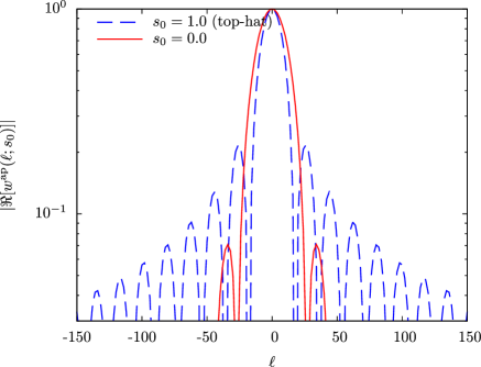
The parameter, $s_{0}$, indicates the width of the region where the apodization is applied, and the prefactor, $w_{1}\equiv 2a[s_{0}+2(1-s_{0})/\pi]$, is used so that $\int_{-\infty}^{\infty}\,ds\,w^{\rm s}(s,s_{0})=1$. In Fig. 1, we show the Fourier counterpart of the above function:

$$w^{\rm s}(\ell;s_{0})=\int_{-\infty}^{\infty}ds\,e^{i\ell s}\,w^{\rm s}(s;s_{0})\,.$$ (44)

The Fourier counterpart with $s_{0}=0.0$ has a high-contrast peak at $\ell=0$ relative to that of the top-hat function ($s_{0}=1.0$). This implies that the function $W^{\rm s}(\hat{\bm{n}};s_{0})$ given by Eq. (43) with $s_{0}=0.0$ would be a better choice to reduce mode coupling, compared to that with $s_{0}=1.0$. From here forward, the fiducial value of parameter, $s_{0}$ in all of our survey boundary apodization is set to $s_{0}=0.0$. In order to see the dependence of this parameter, we also show the case with an intermediate value, $s_{0}=0.5$.

We now construct an apodization function for both the survey boundaries and detected point sources. Let us consider an observed map given on an $S=[-a:a]\times[-a:a]$ plane with $N_{\mathrm{m}}$ detected point sources, each of which we would like to mask. For simplicity, we will use a square mask function, with a length of $r_{\mathrm{m}}$ on each size. We apply an apodizing window function to the observed map, given as

$$W(\hat{\bm{n}};s_{0},t_{0})=\frac{1}{W_{1}(s_{0},t_{0})}W^{\rm s}(\hat{\bm{n}};s_{0})\prod_{i=1}^{N_{\mathrm{m}}}(1-W_{(i)}^{\rm m}(\hat{\bm{n}};t_{0}))\,,$$ (45)

The function, $W^{\rm s}(\hat{\bm{n}};s_{0})$, is used to apodize the edges of the survey region, while the functions $1-W_{(i)}^{\rm m}(\hat{\bm{n}};t_{0})$, apodize the point sources. The factor $W_{1}$ is given by

$$W_{1}(s_{0},t_{0})=\int d^{2}\hat{\bm{n}}\,e^{i\hat{\bm{n}}\cdot\bm{\ell}}W^{\rm s}(\hat{\bm{n}};s_{0})\prod_{i=1}^{N_{\mathrm{m}}}(1-W_{(i)}^{\rm m}(\hat{\bm{n}};t_{0}))\,,$$ (46)

and the functions, $W_{(i)}^{\rm m}(\hat{\bm{n}};t_{0})$ $(i=1,2,\dots,N_{\mathrm{m}})$, are defined as

$$W_{(i)}^{\rm m}(x,y;t_{0})=w_{(i)}^{\rm m}(x-x_{i};t_{0})w_{(i)}^{\rm m}(y-y_{i};t_{0})\,,$$ (47)

with

$$w_{(i)}^{\rm m}(t;t_{0})=\begin{cases}1&|t|<b\\ \sin\left(\dfrac{\pi}{2}\dfrac{b(1+t_{0})-|t|}{bt_{0}}\right)&b\leq|t|<b(1+t_{0})\\ 0&b(1+t_{0})\leq|t|\end{cases}\,.$$ (48)

The positions $(x_{i},y_{i})$ denote the position of $i$-th source mask, and $b=r_{\mathrm{m}}/2$. The parameter, $t_{0}$, indicates the size of the apodization region for each source mask, and, similar to the case of $W^{\rm s}(\hat{\bm{n}};s_{0})$, the Fourier counterpart, $W_{(i)}^{\rm m}(\bm{\ell};t_{0})=\int d^{2}\hat{\bm{n}}\,e^{i\bm{\ell}\cdot\hat{\bm{n}}}\,W_{(i)}^{\rm m}(\hat{\bm{n}};t_{0})$, has a sharp peak at $\bm{\ell}\sim\bm{0}$ for large values of $t_{0}$. If both functions, $W^{\rm s}(\hat{\bm{n}};s_{0})$ and $W_{(i)}^{\rm m}(\hat{\bm{n}};t_{0})$, are sharply peaked at $\bm{\ell}\sim\bm{0}$ in Fourier space, the Fourier transform of $W(\hat{\bm{n}};s_{0},t_{0})$ can be approximated as a delta function.

4.1.2 $C^{-1}$ filtering

The minimum-variance filtering which emerges from likelihood-based derivations of lensing estimators is known as $C^{-1}$ filtering. For the data model of Eq. (8) the inverse-variance filtered multipoles, $\bar{\Theta}_{\bm{\ell}}$, are obtained by solving

$$\left[1+\bm{C}^{1/2}\bm{N}^{-1}\bm{C}^{1/2}\right](\bm{C}^{1/2}\bar{\bm{\Theta}})=\bm{C}^{1/2}\bm{N}^{-1}\hat{\Theta}\,,$$ (49)

where $\bar{\bm{\Theta}}$ is a vector whose components are $\bar{\Theta}_{\bm{\ell}}$, $\bm{C}$ is the covariance of the lensed or unlensed CMB anisotropies with

$$\{\bm{C}\}_{\bm{\ell}_{i},\bm{\ell}_{j}} =\delta_{\bm{\ell}_{i}-\bm{\ell}_{j}}C_{\ell_{i}}^{\Theta\Theta}\,,$$ (50)

and $\bm{N}=\langle\bm{n}^{\dagger}\bm{n}\rangle$ is the covariance matrix for the instrumental noise. The noise covariance matrix in Fourier space is obtained from that in real space as

$$\bm{N}^{-1}=\bm{Y}^{\dagger}\bm{\overline{N}}^{-1}\bm{Y}\,,$$ (51)

where the pointing matrix, $\bm{Y}$, is defined by

$$\{\bm{Y}\}_{\hat{\bm{n}}_{i},\bm{\ell}_{j}}=\exp(i\hat{\bm{n}}_{i}\cdot\bm{\ell}_{j})\,.$$ (52)

The mask is incorporated by setting the noise level of masked pixels to infinity, and therefore the inverse of the noise covariance in real space $\bm{\overline{N}}^{-1}$ to zero for masked pixels. The inversion of the matrix on the left-hand side of Eq. (49) can be numerically costly, but may be evaluated using conjugate descent with careful preconditioning (Smith et al., 2007).

For our $C^{-1}$ results, after applying the $C^{-1}$ filter we additionally apply an apodizing function to account for the survey boundary, given by Eq. (43).

Figure 2: The power spectrum of the mask mean-field, using $100$ Gaussian unlensed map realizations with the standard quadratic estimator (left) and the bias-reduced estimator (right). In each panel, we show the case with diagonal filtering (S-diag, BR-diag), apodization (S-apo, BR-apo), and C-inverse filtered map (S-inv, BR-inv). The black line shows the Monte-Carlo noise, $N^{\phi,(0)}_{\ell}/100$. The multipoles are used up to $\ell_{\mathrm{max}}=3000$. The number and size of masks, $N_{\mathrm{m}}$ and $r_{\mathrm{m}}$, are fixed with $70$ and $10^{\prime}$, respectively; the total fraction of masked area is $\sim 2$%.

Figure 3: Same as Fig. 2 but for $s_{0}=0.5$.

Figure 4: Same as Fig.2, but for $r_{\mathrm{m}}=20^{\prime}$; the total fraction of masked area is $\sim 8$%.

4.2 Mean-field power spectrum

Figure 5: The angular power spectrum of lensing estimator with Gaussian simulation, using the standard quadratic estimator with a perfect subtraction of the mean-field bias (Eq. 6, left panel) and the bias-reduced estimator (Eq. 27, right panel). The mean and error bars of angular power spectrum are computed by $100$ realizations of the simulation.

We now proceed to our numerical results. We start by looking at the power spectrum of the mean-field for both the standard and bias-reduced estimators.

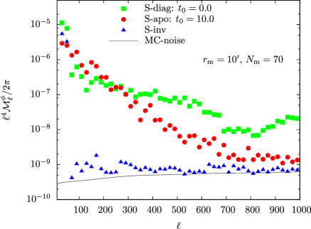
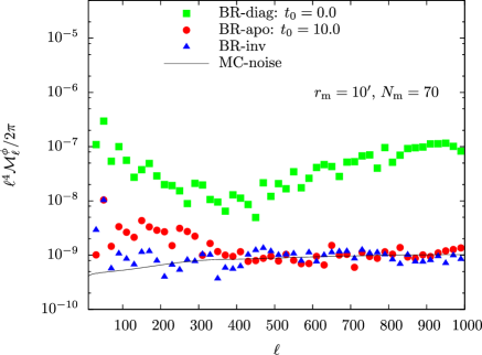
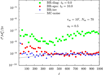
In Fig. 2, we plot the power spectrum

$$\mathcal{M}_{\ell}\equiv\frac{1}{W_{2}}\int\frac{d\varphi_{\bm{\ell}}}{2\pi}\bigg{|}\frac{1}{100}\sum_{i=1}^{100}\hat{x}^{g,i}_{\bm{\ell}}\bigg{|}^{2}\,,$$ (53)

where $\hat{x}^{g,i}_{\bm{\ell}}$ is reconstructed from $i$-th realization of an unlensed Gaussian map without mean-field subtraction, and $W_{2}$ is derived (in analogy to Appendix B) as

$$W_{2} \equiv\int d^{2}\hat{\bm{n}}\,W^{2}(\hat{\bm{n}};s_{0},t_{0})\,.$$ (54)

We construct source masks with $N_{\mathrm{m}}=70$ and $r_{\mathrm{m}}=10^{\prime}$. To show the usefulness of bias-reduced estimator, we compute

• the standard quadratic estimator (Eq. 6), or

• the bias-reduced estimator (Eq. 27),

where the filtering is taken to be

• the diagonal filter with no apodization of source holes ($t_{0}=0$, denoted as S-diag) or

• the diagonal filter with apodized source holes (non-zero $t_{0}$, denoted as S-apo), or

• the inverse-variance filtered map (denoted as S-inv).

As noted above, in all cases we use $s_{0}=0.0$. The results for the bias-reduced estimator are prefixed by “BR”.

It is clear that the mean field bias from the standard quadratic estimator is large particularly on large scales, $\ell\raise 2.9pt\hbox{$\scriptstyle<$}\lower 0.5pt\hbox{$\scriptscriptstyle\sim$}\;500$. For the standard quadratic estimator, the mean-field on large scales still has a large amplitude even with source apodization or $C^{-1}$ filtering. When we use the inverse-variance filtering, the mean-field contribution from source holes is suppressed significantly. This is because the $\bm{\alpha}_{\bm{\ell}}$ term in the estimator (c.f. Eq. 11) in the case of $C^{-1}$ filtering corresponds to Wiener filtering, which is able to reconstruct the component of the masked signal which is due to modes larger than the holes themselves. Most of the power in the CMB gradient is due to scales greater than $r_{\mathrm{m}}=10^{\prime}$, and so this inpainting aspect of the $C^{-1}$ filter significantly reduces the generation of spurious gradients near the source boundary. Even for $C^{-1}$ filtering, however, there exists a mean-field on large scales $\ell\raise 2.9pt\hbox{$\scriptstyle<$}\lower 0.5pt\hbox{$\scriptscriptstyle\sim$}\;100$ due to the survey boundary in the standard estimator. On the other hand, even without source apodization, the bias-reduced estimator suppresses the mean-field significantly. If we use the source apodization or $C^{-1}$ filtering, the mean-field is suppressed significantly, and the amplitude close to the Monte-Carlo noise level.

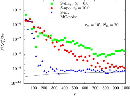
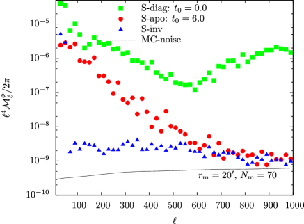
Fig. 3 shows the case with $s_{0}=0.5$. The mean-field bias increases compared to the case with $s_{0}=0.0$, because of the residuals of survey boundary effect. This implies that, under the apodization function given in Eq. (43), the mean-field bias from survey boundary effect would be minimized if we choose $s_{0}=0.0$.

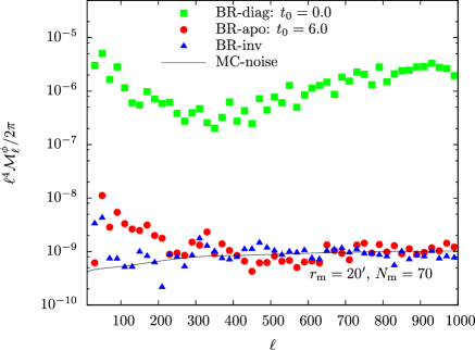
In Fig. 4, we show the case with $r_{\mathrm{m}}=20^{\prime}$. Even in this case, for standard quadratic estimator, either the source apodization or $C^{-1}$ filtering suppresses the mean field significantly compared to the case without these two filtering methods, but, similar to $r_{\mathrm{m}}=10^{\prime}$, there are still large mean field at large scales. For the bias-reduced estimator, the mean field is suppressed down to the Monte-Carlo noise floor.

Figure 6: The error of estimator in the presence of uncertainties in the subtraction of mean-field bias. The points show the error in the case with apodization (red) or $C^{-1}$ filtering, assuming $\epsilon=0.1$ or $\epsilon=0.01$. For comparison, we also show the error of bias-reduced estimator. All errors are normalized by the case in the absence of uncertainties in the mean-field subtraction.

Figure 7: The angular power spectrum of the bias-reduced estimator for pseudo-scalar lensing potential, in the case with $N_{\mathrm{m}}=70$ and $r_{\mathrm{m}}=10^{\prime}$.

Figure 8: Same as Fig. 5, but using simulated lensed temperature maps. The gray lines show the theoretical reconstruction noise bias, $N_{\ell}^{\phi,(0)}$.

4.3 Power spectrum of lensing estimator

Next, we show the power spectrum of the lensing estimator computed from unlensed Gaussian simulations, i.e., the reconstruction noise bias. The reconstruction noise bias of the $i$-th realization map is computed as

$$\hat{N}_{\ell}^{xx,i}=\frac{1}{W_{4}}\int\frac{d\varphi_{\bm{\ell}}}{2\pi}|\hat{x}^{g,i}_{\bm{\ell}}|^{2}\,,$$ (55)

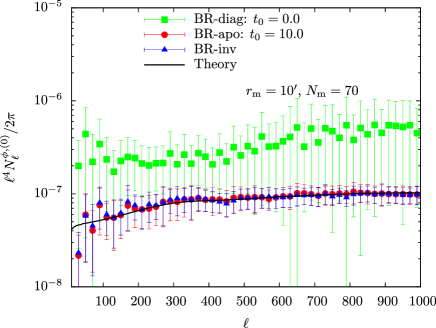
and then the mean of $100$ realizations is compared with the full-sky, diagonal filtering expectation. Note that, for the reduced bias estimator, the noise bias is modified, i.e., the standard reconstruction noise bias divided by $(1-R_{\ell}^{\phi,M}R_{\ell}^{M,\phi})$.

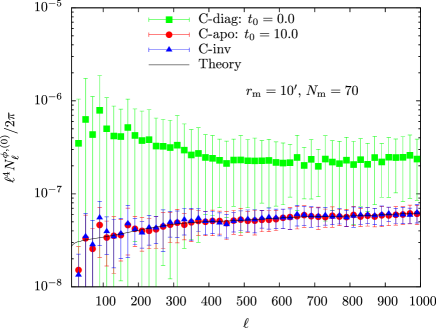
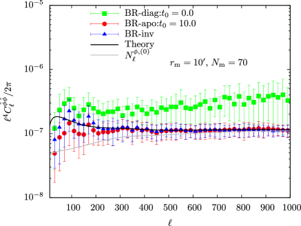
In Fig. 5, we show the reconstruction noise bias, for the same cases as shown in Fig. 2. We note that for both apodization and $C^{-1}$ filtering, the reconstruction noise bias agrees well with the analytical approximation using either the standard estimator (after a perfect mean-field subtraction) or the bias-reduced estimator.

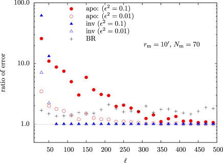
Now we turn to discuss the error of the estimators in the presence of incomplete mean-field subtraction in the conventional approach. The advantage of the bias-reduced approach is that it may be less strongly sensitive on how accurately we model the statistics of the underlying fluctuations. In the above analysis, although the error bars for the bias-reduced result are slightly larger than those for the standard result, the uncertainties in the mean-filed bias are completely ignored, and inclusion of other possible sources for mean-field bias degrades the accuracy in the standard approach. To see this, we consider a case with uncertainties in the mean-field bias generated by, e.g., calibration error as discussed in the previous section, and the resultant estimator is parametrized by a small parameter, $\epsilon$, as

$$\hat{\phi}^{\rm C}_{\bm{\ell}}\to\hat{\phi}^{\rm C}_{\bm{\ell}}+\epsilon\langle\hat{\phi}^{\rm S}_{\bm{\ell}}\rangle\,.$$ (56)

Fig. 6 shows the errors taking into account this uncertainty normalized by the case for a perfect subtraction of mean-field bias, $1+\epsilon^{2}\mathcal{M}_{\ell}^{\phi}/N_{\ell}^{\phi,(0)}$, where the power spectrum of mean-field bias, $\mathcal{M}_{\ell}$, is computed for $N_{\mathrm{m}}=70$ and $r_{\mathrm{m}}=10^{\prime}$. We also show the errors expected from the bias-reduced estimator divided by those from the standard approach without uncertainties in the mean-field subtraction. As clearly shown, the uncertainties for the standard approach are significant on large scales ($\ell\raise 2.9pt\hbox{$\scriptstyle<$}\lower 0.5pt\hbox{$\scriptscriptstyle\sim$}\;100$), where the lensing signals are dominated, compared to that for the bias-reduced estimator.

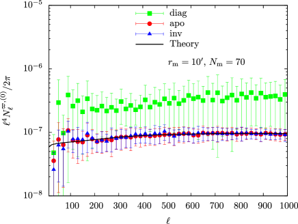
In Fig. 7, we show the pseudo-scalar lensing potential. The reconstruction noise of the pseudo-scalar lensing potential is modified and the normalization is biased by the mode coupling due to the presence of sky cuts and masks. Note that there is no characteristic feature at large scales as there is for the scalar-lensing potential. This is because the estimator of the pseudo-scalar lensing potential is not significantly biased by the masking mean-field, as discussed in Sec. 3. Similar to the case with bias-reduced estimator of the scalar-lensing potential, using source apodization, the reconstruction noise agrees well with the analytical prediction for small source holes.

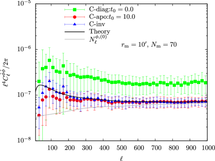
Finally, in Fig. 8, to see how well the bias can be reduced even in the presence of lensing field, as well as how well the estimator normalization is described by the full-sky equation, we show the angular power spectrum of lensing estimator, computed from Eq. (55) but using the estimator reconstructed from $i$-th realization of simulated lensed map. The theoretical prediction is the sum of the reconstruction noise, $N_{\ell}^{x,(0)}=A_{\ell}^{x}$, and the power spectrum of scalar-lensing potential, $C_{\ell}^{\phi\phi}$. The results are similar to that in the case with the unlensed Gaussian simulation.

5 Summary

We have discussed methods for removing the “mean-field” and “reconstruction noise” biases which must be accounted for in CMB lens reconstruction. Our approach focuses on estimating these biases directly from the data itself, reducing our sensitivity to the sky model which is otherwise needed to determine them. We performed numerical tests of the mean-field reduction approach for several different choices of filtering, finding it particularly useful for the reduction of the large-scale component of the mean-field.

In our analysis, we have focused on the temperature fluctuations, but upcoming and next-generation CMB experiments will also provide information on the polarization. The polarization anisotropies are a more sensitive probe of lensing effects and thus the lensing reconstruction from realistic polarization maps is also worth investigating. The method investigated in this paper may be also applicable to the polarization maps, and the usefulness of our method to the lensing reconstruction from polarization maps will be explored in our future work (Namikawa et al in prep.).

Our simulation results of the lensed temperature anisotropies are available as numeric tables upon request (contact takahasi@cc.hirosaki-u.ac.jp).

Appendix A Numerical simulation of lensed CMB maps

In this section, we describe our method to generate lensed CMB maps, based on the ray-tracing of large-scale structure simulations (e.g., Sato et al. 2009; Takahashi et al. 2011).

Fig. 9 shows a schematic picture of our ray-tracing simulation. We have multiple lens planes but use a flat-sky approximation. The horizontal axis is the comoving distance $r$ from the observer. The thick vertical lines are the lens and source planes, which are placed at equal-distance intervals of $L$, and located at $r=(i-1/2)\times L$ with an integer $i=1,2,\cdots,N$. Here, $i=N$ corresponds to the source plane. We place the source plane at the last scattering surface $(z_{s}=1090)$. The distance to the last scattering surface is $r_{\rm LSS}=r(z_{s}=1090)=9900h^{-1}$Mpc in our fiducial cosmological model. We place $19$ lens planes up to the last scattering surface, i.e., we set $N=20$. We determine the interval $L$ from the distance to the last scattering surface divided by the number of lens planes, $L=r_{\rm LSS}/(N-1/2)=r_{\rm LSS}/(20-1/2)=507.6h^{-1}$Mpc. Light rays are emitted from the observer and are deflected at each lens plane before reaching the source plane. In our simulation, the field of view is $10\times 10$ deg². We impose a periodic boundary condition on the lens planes.

Figure 9: A schematic picture of our ray-tracing simulation. The horizontal axis is the comoving distance $r$ from the observer. The vertical thick lines denote the positions of the lens planes and the source plane, which are located at $r=(i-1/2)\times L$ with $i=1,2,\cdots,N$. Here, we set $N=20$. We have multiple lens planes but use the flat-sky approximation. Light rays are emitted from the observer and are deflected at the lens planes before reaching the source plane. The field of view is $10\times 10$ deg².

A.1 $N$-body Simulations

In order to obtain the particle distribution and the gravitational potential on the lens planes, we run $N$-body simulations in a cubic box, and then project the particle positions into two dimensions perpendicular to the line-of-sight. We use the numerical simulation code Gadget2 (Springel et al., 2001; Springel, 2005). We generate the initial conditions based on the second-order Lagrangian perturbation theory (2LPT; Crocce et al. 2006; Nishimichi et al. 2009) with the initial linear power spectrum calculated by CAMB. We employ $1024^{3}$ dark matter particles in the simulation box of $L=507.6$ $h^{-1}$Mpc on a side. The initial redshift is $z_{\rm init}=70$, and we dump the outputs (the particle positions) at the redshifts corresponding to the positions of the lens planes $r=L\times(i-1/2)$, shown in Fig. 9. The softening length is fixed to be $5\%$ of the mean particle separations, which correspond to $25$ $h^{-1}$kpc. We prepare five independent realizations to reduce the sample variance.

A.2 Ray-tracing Simulations

We briefly explain the procedure to trace light rays through $N$-body data and obtain the maps of the lensing fields on the source plane (see also, e.g., Sato et al. 2009; Takahashi et al. 2011). We use the code RAYTRIX (Hamana & Mellier, 2001) which follows the standard multiple lens plane algorithm. In the standard multiple lens plane algorithm, the distance between observer and source galaxies is divided into several intervals. In our case, as shown in Fig. 9, we adopt a fixed interval whose value is the same as simulation box $L$ on a side. Particle positions are projected onto two dimensional lens planes ($xy$, $yz$ ,$zx$ planes) every $L$. Using the Triangular-Shaped Cloud method (Hockney & Eastwood, 1988), we assign the particles onto $N_{g}^{2}$ grids in lens planes, then compute the projected density contrast at each plane. We use $N_{g}^{2}=2048^{2}$ throughout this paper. The two-dimensional gravitational potential is solved via the Poisson equation using a Fast Fourier Transform. Finally, two dimensional sky maps of the convergence, shear, and angular positions of light rays are obtained by solving the evolution equation of Jacobian matrix along the light-ray path which is obtained by solving the multiple lens equation. At high redshifts ($z>12$), the density fluctuations are very small and give only $<10\%$ contribution to the angular power spectrum of the lensing potential at the multipole $\ell=100-1000$ (see Lewis & Challinor 2006). Hence, at high redshifts ($z>12$) we do not include the density fluctuations in our calculation. We solve the multiple lens equation up to $z=12$ and further redshifts the light rays are assumed to propagate in straight lines.

We prepare $100$ realizations by randomly choosing the projecting direction and shifting the two dimensional positions. In each realization, we emit $1024^{2}$ light-rays in the field-of-view $10\times 10$ deg². Then, the angular resolution is $10$deg$/1024\simeq 0.6^{\prime}$.

Figure 10: The power spectrum of the scalar lensing potential at the last scattering surface ($z=1090$). The dots with error bars are our ray-tracing simulation results calculated from the $100$ retaliations of $10\times 10$ deg² convergence maps. The black curve is the theoretical prediction.

In order to check the accuracy of our ray-tracing simulation, we calculate the power spectrum of scalar lensing potential and compare it with the theoretical model. Fig. 10 shows the power spectrum, $\ell^{4}C_{\ell}^{\phi\phi}/2\pi$, as a function of multipole $\ell$ at the last scattering surface ($z=1090$). The dots with error bars are the simulation results calculated from the $100$ realizations of $10\times 10$ deg² convergence maps. The black curve is the theoretical prediction in which the power spectrum of scalar lensing potential is given by the projected (three-dimensional) matter power spectrum weighted with the radial lensing kernel along the line-of-sight (e.g., Bartelmann & Schneider 2001). Here, we use the halo-fit model (Smith et al., 2003) to calculate the non-linear power spectrum. As clearly seen in the figure, our simulation results agree with the theoretical model very well.

A.3 Lensed CMB Temperature Map

In this subsection, we introduce our procedure for making lensed CMB temperature maps. We prepare these maps as follows:

1. We obtain the power spectrum of the unlensed CMB temperature fluctuations using CAMB.

2. We make an unlensed temperature map on a square $\sqrt{4\pi}$ radian ($\simeq 203$ deg) on a side assuming Gaussian fluctuations based on the unlensed power spectrum. The angular resolution of the temperature fluctuations is set to be $10$ deg$/1024\simeq 0.6^{\prime}$. We prepare $100$ such unlensed maps.

3. Finally, we calculate the deflection angle ${\bm{d}}(\hat{\bm{n}})$ at the angular position $\hat{\bm{n}}$ using the ray-tracing simulation for the $1024^{2}$ light rays. Then, we obtain the lensed temperature map by shifting the positions $\hat{\bm{n}}\rightarrow\hat{\bm{n}}+{\bm{d}}(\hat{\bm{n}})$ on the unlensed map, according to Eq. (1). We have $100$ lensed CMB temperature maps of $10\times 10$ deg² with $1024^{2}$ grids.

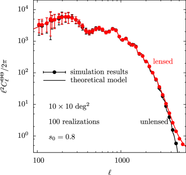
We calculate the power spectrum from the $100$ lensed CMB temperature maps, and the result is shown in Fig. 11. The figure shows the angular power spectrum of lensed temperature fluctuations as a function of multipole $\ell$. The dots with error bars are the mean values and the dispersions calculated from the $100$ realizations. We use $s_{0}=0.8$ in the apodization. The red symbols are the lensed power spectrum, while the black symbols are unlensed. The solid curves are the theoretical prediction calculated by CAMB. Our simulation results agree with the theoretical predication very well.

Figure 11: The lensed CMB temperature power spectrum. The red symbols are the lensed power spectrum, while the black symbols are unlensed one. The dots with error bars are our simulation results calculated from the $100$ realizations of $10\times 10$ deg² lensed maps. Here, we use $s_{0}=0.8$ in the apodization. The solid curves are the results from CAMB.

Appendix B Apodized Normalization

Apodization/masking leads to a change in the angular power spectrum of the lensing estimator. Here we derive the appropriate correction to the normalization of the estimator power spectrum.

Substituting Eq. (17) into Eq. (6), the estimator in the presence of an general window function is given as

$$\hat{x}_{\bm{\ell}} =\int\frac{d^{2}\bm{L}}{(2\pi)^{2}}{F}^{x}_{\bm{\ell},\bm{L}}\int\frac{d^{2}\bm{\ell}_{1}^{\prime}{\mathstrut}}{(2\pi)^{2}}\int\frac{d^{2}\bm{\ell}_{2}^{\prime}{\mathstrut}}{(2\pi)^{2}}W_{\bm{L}-\bm{\ell}_{1}^{\prime}{\mathstrut}}W_{\bm{\ell}-\bm{L}-\bm{\ell}_{2}^{\prime}{\mathstrut}}\hat{\Theta}_{\bm{\ell}_{1}^{\prime}{\mathstrut}}\hat{\Theta}_{\bm{\ell}_{2}^{\prime}{\mathstrut}}\,,$$ (57)

where we define ${F}^{x}_{\bm{\ell},\bm{L}}={A}_{\ell}^{x}{f}^{x}_{\bm{\ell},\bm{L}}/2\hat{C}_{L}^{\Theta\Theta}\hat{C}_{|\bm{\ell}-\bm{L}|}^{\Theta\Theta}$. From the above equation, the angular power spectrum of the estimator becomes

$$\langle|\hat{x}_{\bm{\ell}}|^{2}\rangle=\int\frac{d^{2}\bm{L}}{(2\pi)^{2}}\int\frac{d^{2}\bm{L}^{\prime}{\mathstrut}}{(2\pi)^{2}}{F}^{x}_{\bm{\ell},\bm{L}}{F}^{x}_{\bm{\ell},\bm{L}^{\prime}{\mathstrut}}\\ \times\int\frac{d^{2}\bm{\ell}_{1}}{(2\pi)^{2}}\int\frac{d^{2}\bm{\ell}_{2}}{(2\pi)^{2}}\int\frac{d^{2}\bm{\ell}_{3}}{(2\pi)^{2}}\int\frac{d^{2}\bm{\ell}_{4}}{(2\pi)^{2}}\\ \times W_{\bm{L}-\bm{\ell}_{1}}W_{\bm{\ell}-\bm{L}-\bm{\ell}_{2}}W_{\bm{L}-\bm{\ell}_{3}}W_{\bm{\ell}-\bm{L}-\bm{\ell}_{4}}\\ \times\langle\hat{\Theta}_{\bm{\ell}_{1}}\hat{\Theta}_{\bm{\ell}_{2}}\hat{\Theta}_{-\bm{\ell}_{3}}\hat{\Theta}_{-\bm{\ell}_{4}}\rangle\,,$$ (58)

where we use $\hat{\Theta}^{*}_{\bm{L}}=\hat{\Theta}_{-\bm{L}}$. Note that the statistical anisotropy of lensed fields restrict the integral of Fourier modes, $\bm{\ell}_{1}$, $\bm{\ell}_{2}$, $\bm{\ell}_{3}$ and $\bm{\ell}_{4}$, to the case with $\bm{\ell}_{1}+\bm{\ell}_{2}-\bm{\ell}_{3}-\bm{\ell}_{4}=\bm{0}$, the delta function, $\delta_{\bm{\ell}_{1}+\bm{\ell}_{2}-\bm{\ell}_{3}-\bm{\ell}_{4}}$, is multiplied in the integrand of the above equation. If the window functions behave as the delta function, the above equation reduces to

$$\langle|\hat{x}_{\bm{\ell}}|^{2}\rangle\simeq\int\frac{d^{2}\bm{L}}{(2\pi)^{2}}\int\frac{d^{2}\bm{L}^{\prime}{\mathstrut}}{(2\pi)^{2}}{F}^{x}_{\bm{\ell},\bm{L}}{F}^{x}_{\bm{\ell},\bm{L}^{\prime}{\mathstrut}}\\ \times\langle\hat{\Theta}_{\bm{L}}\hat{\Theta}_{\bm{\ell}-\bm{L}}\hat{\Theta}_{-\bm{L}}\hat{\Theta}_{-\bm{\ell}+\bm{L}}\rangle W_{4}\,.$$ (59)

The quantity $W_{4}$ is defined by

$$W_{4}\equiv\int\frac{d^{2}\bm{\ell}_{1}}{(2\pi)^{2}}\int\frac{d^{2}\bm{\ell}_{2}}{(2\pi)^{2}}\int\frac{d^{2}\bm{\ell}_{3}}{(2\pi)^{2}}\int\frac{d^{2}\bm{\ell}_{4}}{(2\pi)^{2}}\\ \times W_{\bm{L}-\bm{\ell}_{1}}W_{\bm{\ell}-\bm{L}-\bm{\ell}_{2}}W_{\bm{L}-\bm{\ell}_{3}}W_{\bm{\ell}-\bm{L}-\bm{\ell}_{4}}\delta_{\bm{\ell}_{1}+\bm{\ell}_{2}-\bm{\ell}_{3}-\bm{\ell}_{4}}$$ (60)

which reduces to

$$W_{4} = \prod_{i=1}^{4}\int\frac{d^{2}\bm{\ell}_{j}^{\prime}{\mathstrut}}{(2\pi)^{2}}W_{\bm{\ell}_{j}^{\prime}{\mathstrut}}\int d^{2}\hat{\bm{n}}\,e^{i\hat{\bm{n}}\cdot(\bm{\ell}_{1}+\bm{\ell}_{2}-\bm{\ell}_{3}-\bm{\ell}_{4})}$$ (61)

$$= \int d^{2}\hat{\bm{n}}\,W^{4}(\hat{\bm{n}})\,.$$

Eq. (59) means that the power spectrum of reconstructed estimator from finite-size masked map is equal to that from ideal map multiplied by the quantity $W_{4}$.

References

- Bartelmann & Schneider (2001) Bartelmann M., Schneider P., 2001, Phys. Rep., 340, 291
- Bleem et al. (2012) Bleem L., van Engelen A., Holder G., Aird K., Armstrong R., et al., 2012, Astrophys. J., 753, L9
- Bucher et al. (2012) Bucher M., Carvalho C. S., Moodley K., Remazeilles M., 2012, Phys. Rev. D, 85, 043016
- Carvalho & Tereno (2011) Carvalho C. S., Tereno I., 2011, Phys. Rev. D, 84, 063001
- Cooray et al. (2005) Cooray A., Kamionkowski M., Caldwell R. R., 2005, Phys. Rev. D, 71, 123527
- Crocce et al. (2006) Crocce M., Pueblas S., Scoccimarro R., 2006, Mon. Not. Roy. Astron. Soc., 373, 369
- Das & Bode (2008) Das S., Bode P., 2008, Astrophys. J., 682, 1
- Das et al. (2011) Das S., Sherwin B. D., et al., 2011, Phys. Rev. Lett., 107, 021301
- de Putter et al. (2009) de Putter R., Zahn O., Linder E. V., 2009, Phys. Rev. D, 79, 065033
- Dvorkin & Smith (2009) Dvorkin C., Smith K. M., 2009, Phys. Rev. D, 79, 043003
- Feng et al. (2012) Feng C., Aslanyan G., Manohar A. V., Keating B., Paar H. P., Zahn O., 2012, Phys. Rev. D, 86, 063519
- Feng et al. (2011) Feng C., Keating B., Paar H. P., Zahn O., 2011, Phys. Rev. D, 85, 043513
- Hamana & Mellier (2001) Hamana T., Mellier Y., 2001, Mon. Not. Roy. Astron. Soc., 327, 169
- Hanson et al. (2011) Hanson D., Challinor A., Efstathiou G., Bielewicz P., 2011, Phys. Rev. D, 83, 043005
- Hanson & Lewis (2009) Hanson D., Lewis A., 2009, Phys. Rev. D, 80, 063004
- Hanson et al. (2010) Hanson D., Lewis A., Challinor A., 2010, Phys. Rev. D, 81, 103003
- Hanson et al. (2009) Hanson D., Rocha G., Gorski K., 2009, Mon. Not. Roy. Astron. Soc., 400, 2169
- Hirata et al. (2008) Hirata C. M., Ho S., Padmanabhan N., Seljak U., Bahcall N. A., 2008, Phys. Rev. D, 78, 043520
- Hirata & Seljak (2003a) Hirata C. M., Seljak U., 2003a, Phys. Rev. D, 67, 043001
- Hirata & Seljak (2003b) Hirata C. M., Seljak U., 2003b, Phys. Rev. D, 68, 083002
- Hockney & Eastwood (1988) Hockney R. W., Eastwood J., 1988, Computer simulation using particles. Taylor & Francis
- Hu (2001) Hu W., 2001, Phys. Rev. D, 64, 083005
- Hu (2002) Hu W., 2002, Phys. Rev. D, 65, 023003
- Hu & Okamoto (2002) Hu W., Okamoto T., 2002, Astrophys. J., 574, 566
- Jeong et al. (2009) Jeong D., Komatsu E., Jain B., 2009, Phys. Rev. D, 80, 123527
- Kesden et al. (2003) Kesden M. H., Cooray A., Kamionkowski M., 2003, Phys. Rev. D, 67, 123507
- Komatsu et al. (2011) Komatsu E., et al., 2011, Astrophys. J. Suppl., 192, 18
- Lesgourgues & Pastor (2006) Lesgourgues J., Pastor S., 2006, Phys. Rep., 429, 307
- Lewis & Challinor (2006) Lewis A., Challinor A., 2006, Phys. Rep., 429, 1
- Lewis et al. (2011) Lewis A., Challinor A., Hanson D., 2011, JCAP, 1103, 018
- Lewis et al. (2000) Lewis A., Challinor A., Lasenby A., 2000, Astrophys. J., 538, 473
- Namikawa et al. (2010) Namikawa T., Saito S., Taruya A., 2010, JCAP, 1012, 027
- Namikawa et al. (2012) Namikawa T., Yamauchi D., Taruya A., 2012, JCAP, 1201, 007
- Nishimichi et al. (2009) Nishimichi T., Shirata A., Taruya A., Yahata K., Saito S., et al., 2009, PASJ, 61, 321
- Okamoto & Hu (2003) Okamoto T., Hu W., 2003, Phys. Rev. D, 67, 083002
- Perotto et al. (2010) Perotto L., Bobin J., Plaszczynski S., Starck J.-L., Lavabre A., 2010, Astron. Astrophys., 519, A4
- Plaszczynski et al. (2012) Plaszczynski S., Lavabre A., Perotto L., Starck J.-L., 2012, Astron. Astrophys., 544, A27
- Regan et al. (2010) Regan D., Shellard E., Fergusson J., 2010, Phys. Rev. D, 82, 023520
- Sato et al. (2009) Sato M., Hamana T., Takahashi R., Takada M., Yoshida N., Matsubara T., Sugiyama N., 2009, Astrophys. J., 701, 945
- Seljak & Zaldarriaga (1999) Seljak U., Zaldarriaga M., 1999, Phys. Rev. Lett., 82, 2636
- Sherwin & Das (2010) Sherwin B. D., Das S., 2010
- Sherwin et al. (2012) Sherwin B. D., Das S., Hajian A., Addison G., Bond J. R., et al., 2012, Phys. Rev. D, 86, 083006
- Smith et al. (2007) Smith K. M., Zahn O., Dore O., 2007, Phys. Rev. D, 76, 043510
- Smith et al. (2003) Smith R. E., et al., 2003, Mon. Not. Roy. Astron. Soc., 341, 1311
- Souradeep & Ratra (2001) Souradeep T., Ratra B., 2001, Astrophys. J., 560, 28
- Springel (2005) Springel V., 2005, Mon. Not. Roy. Astron. Soc., 364, 1105
- Springel et al. (2001) Springel V., Yoshida N., White S. D., 2001, New Astron., 6, 79
- Takahashi et al. (2011) Takahashi R., Oguri M., Sato M., Hamana T., 2011, Astrophys. J., 742, 15
- Takeuchi et al. (2012) Takeuchi Y., Ichiki K., Matsubara T., 2012, Phys. Rev. D, 85, 043518
- van Engelen et al. (2012) van Engelen A., Keisler R., Zahn O., Aird K., Benson B., et al., 2012, Astrophys. J., 756, 142
- Yamauchi et al. (2012) Yamauchi D., Namikawa T., Taruya A., 2012, JCAP, 1210, 030
- Yamauchi et al. (2012) Yamauchi D., Takahashi K., Sendouda Y., Yoo C.-M., 2012, Phys. Rev. D, 85, 103515
- Zaldarriaga & Seljak (1999) Zaldarriaga M., Seljak U., 1999, Phys. Rev. D, 59, 123507