Trapping of a particle in a short-range harmonic potential well

Abstract

Eigenstates of a particle in a localized and unconfined harmonic potential well are investigated. Effects due to the variation of the potential parameters as well as certain results from asymptotic expansions are discussed.


Key words: short-range harmonic oscillator; bound states; confluent hypergeometric function

1 Introduction

Systems confined have received considerable attention in quantum mechanics. The hydrogen atom confined in a spherical enclosure was first analyzed in 1937 [1], the restricted rotator in 1940 [2] and the harmonic oscillator in 1943 [3]. Since then the one-dimensional oscillator immersed in an infinite square potential has received some attention [4]-[8]. It should also be mentioned that two different cases for a sort of one-dimensional half-oscillator have also been reported, one of them bound by an infinite wall [7], [9] and the other one by a finite step potential [9]. Recently, the D-dimensional confined harmonic oscillator appeared in the literature [10]-[12].

The square well potential is an unconfined potential with vertical walls that has been used to model band structure in solids [13] and semiconductor heterostructures [14]-[17]. The use of a quantum well with sloping sides might be of interest to refine those models. As a matter of fact, a sort of localized triangular potential has been an item of recent practical [18]-[19] and theoretical [20]-[23] investigations.

In this paper we consider the bound-state problem for a particle immersed in an one-dimensional harmonic potential which vanishes outside a finite region. To the best of our knowledge this sort of trapping has never been solved. By using confluent hypergeometric functions the process of solving the Schrödinger equation for the eigenenergies is transmuted into the simpler and more efficient process of solving a transcendental equation. Such as for the well-known square potential, a graphical method provides some qualitative conclusions about the spectrum of this short-range potential well. Approximate analytical results for the special cases of low-lying states and high-lying states are obtained with the help of asymptotic representations and limiting forms for the confluent hypergeometric function. It is shown that the localized harmonic potential yields the full harmonic potential and the square well potential as limiting cases. Although the quantization condition has no closed form expressions in terms of simpler functions, the exact computation of the allowed eigenenergies can be done easily with a root-finding procedure of a symbolic algebra program. Proceeding in this way, the whole bound-state spectrum is found. Nevertheless, our purpose is to investigate the basic nature of the phenomena without entering into the details involving specific applications. In other words, the aim of this paper is to explore a simple system which can be of help to see more clearly what is going on into the details of a more specialized and complex circumstance such as that one in Ref. [24].

2 The particle in a short-range harmonic potential well

Let us write the short-range harmonic potential well as

$$V(x) = \frac{1}{2}m\omega^{2}\left(x^{2}-rL^{2}\right)\left[\theta\left(x+L\right)-\theta\left(x-L\right)\right]$$ (7)

$$= \left\{\begin{array}[]{c}\frac{1}{2}m\omega^{2}\left(x^{2}-rL^{2}\right)\\ \\ 0\end{array}\begin{array}[]{c}{\textrm{for }}|x|<L\\ \\ {\textrm{for }}|x|>L\end{array}\right.$$

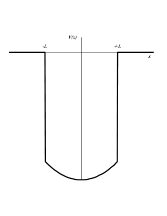
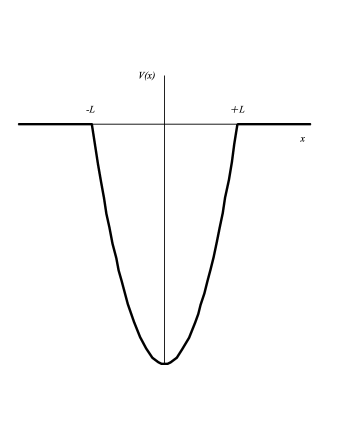
where $\theta\left(x\right)$ is the Heaviside function, $2L$ is the range of the potential, $m$ is the mass of the particle and $\omega$ is the classical frequency of the oscillator. The parameter $r=V(0)/[V(0)-V(L)]$ characterizes four different profiles for the potential as illustrated in Fig. 1. This potential admits scattering states (with $E>0$) and bound states (with $V(0)<E<0$ and $r>0$). In what follows we will consider the bound-state problem.

Let us introduce the new variable

$$z=\alpha\,x,\quad\alpha=\sqrt{\frac{2m\omega}{\hslash}}$$ (8)

so that, for $|x|<L$, the Schrödinger equation

$$\frac{d^{2}\psi(x)}{dx^{2}}+\frac{2m}{\hslash^{2}}\left[E-V\left(x\right)\right]\psi(x)=0$$ (9)

turns into the dimensionless form

$$\frac{d^{2}\psi(z)}{dz^{2}}-\left(\frac{z^{2}}{4}+a\right)\psi(z)=0$$ (10)

where

$$a=\frac{V(0)-E}{\hslash\omega}$$ (11)

The general solution for Eq. (10) can be written as a superposition of definite-parity functions [25]

$$\psi=c_{e}\,y_{1}(a,z)+c_{o}\,y_{2}(a,z)$$ (12)

where

$$y_{1}(a,z)=e^{-z^{2}/4}\,M\left(\frac{a}{2}+\frac{1}{4},\frac{1}{2},\frac{z^{2}}{2}\right)$$

$$y_{2}(a,z)=e^{-z^{2}/4}\,z\,M\left(\frac{a}{2}+\frac{3}{4},\frac{3}{2},\frac{z^{2}}{2}\right)$$ (13)

where $M(a,b,z)=\,_{1}F_{1}\left(a;b;z\right)$ is the confluent hypergeometric function (Kummer’s function)

$$M(a,b,z)=\frac{\Gamma\left(b\right)}{\Gamma\left(a\right)}\sum_{n=0}^{\infty}\frac{\Gamma\left(a+n\right)}{\Gamma\left(b+n\right)}\,\frac{z^{n}}{n!}$$ (14)

$\Gamma\left(z\right)$ is the gamma function, and $c_{e}$ and $c_{o}$ are arbitrary constants. For $x>L$, the evanescent free-particle solution ($\psi$ must vanish as $x\rightarrow\infty$) is expressed as

$$\psi=c\,e^{-kx}$$ (15)

where $c$ is an arbitrary constant and

$$k=\sqrt{\frac{-2mE}{\hslash^{2}}}=\frac{z_{L}^{2}}{L}\sqrt{\frac{r}{4}+\frac{a}{z_{L}^{2}}}$$ (16)

Here,

$$z_{L}=\alpha L=\sqrt{2}\,\frac{\sqrt{\omega}L}{\sqrt{\hslash/m}}$$ (17)

is the value of $z$ at $x=L$. Because $V\left(-x\right)=V\left(x\right)$, the Schrödinger equation is invariant under space inversion ($x\rightarrow-x$) and so we can choose solutions with definite parities. The even ($\psi_{e}$) and odd ($\psi_{o}$) parity eigenfunctions on the entire $x$-axis can be written as

$$\psi_{e}\left(x\right) = c_{e}\,e^{-\alpha^{2}x^{2}/4}\,M\left(\frac{a}{2}+\frac{1}{4},\frac{1}{2},\frac{\alpha^{2}x^{2}}{2}\right)\left[\theta\left(x+L\right)-\theta\left(x-L\right)\right]$$ (18)

$$+\,c\,e^{-k|x|}\left[\theta\left(x-L\right)+\theta\left(-x-L\right)\right]$$

$$\psi_{o}\left(x\right) = c_{o}\,\alpha\,x\,e^{-\alpha^{2}x^{2}/4}\,M\left(\frac{a}{2}+\frac{3}{4},\frac{3}{2},\frac{\alpha^{2}x^{2}}{2}\right)\left[\theta\left(x+L\right)-\theta\left(x-L\right)\right]$$ (19)

$$+\,c\,e^{-k|x|}\left[\theta\left(x-L\right)-\theta\left(-x-L\right)\right]$$

The even parity solutions satisfy the homogeneous Neumann condition at the origin ($d\psi(x)/dx|_{x=0}=0$) and the odd ones the homogeneous Dirichlet condition ($\psi(0)=0$). In this circumstance it is enough to concentrate our attention on the positive side of the $x$-axis and use the continuity of $\psi(x)$ and $d\psi(x)/dx$ at $x=L$. Making use of the recurrence formulas involving $y_{1}$ and $y_{2}$ defined in (13) [25]

$$\frac{dy_{1}(a,z)}{dz}+\frac{z}{2}\,y_{1}(a,z)=\left(a+\frac{1}{2}\right)y_{2}(a+1,z)$$

$$\frac{dy_{2}(a,z)}{dz}+\frac{z}{2}\,y_{2}(a,z)=y_{1}(a+1,z)$$ (20)

one has as a result

$$\frac{d\psi}{dx} = \alpha e^{-z^{2}/4}\left\{c_{e}\,z\left[\left(a+\frac{1}{2}\right)M\left(\frac{a}{2}+\frac{5}{4},\frac{3}{2},\frac{z^{2}}{2}\right)-\frac{1}{2}M\left(\frac{a}{2}+\frac{1}{4},\frac{1}{2},\frac{z^{2}}{2}\right)\right]\right.$$ (21)

$$+\left.c_{o}\left[M\left(\frac{a}{2}+\frac{3}{4},\frac{1}{2},\frac{z^{2}}{2}\right)-\frac{z^{2}}{2}M\left(\frac{a}{2}+\frac{3}{4},\frac{3}{2},\frac{z^{2}}{2}\right)\right]\right\}$$

The continuity of $\psi$ at $x=L$ says that

$$c\,e^{-kL}$$ (22)

is equal to

$$c_{e}\,e^{-z_{L}^{2}/4}\,M\left(\frac{a}{2}+\frac{1}{4},\frac{1}{2},\frac{z_{L}^{2}}{2}\right)$$ (23)

for even parity solutions, and equal to

$$c_{o}\,e^{-z_{L}^{2}/4}z_{L}\,M\left(\frac{a}{2}+\frac{3}{4},\frac{3}{2},\frac{z_{L}^{2}}{2}\right)$$ (24)

for odd parity solutions. Matching $d\psi/dx$ at $x=L$ makes

$$-kc\,e^{-kL}$$ (25)

equal to

$$c_{e}\,\alpha\,e^{-z_{L}^{2}/4}\,z_{L}\left[\left(a+\frac{1}{2}\right)M\left(\frac{a}{2}+\frac{5}{4},\frac{3}{2},\frac{z_{L}^{2}}{2}\right)-\frac{1}{2}M\left(\frac{a}{2}+\frac{1}{4},\frac{1}{2},\frac{z_{L}^{2}}{2}\right)\right]$$ (26)

for even parity solutions, and equal to

$$c_{o}\,\alpha\,e^{-z_{L}^{2}/4}\,\left[M\left(\frac{a}{2}+\frac{3}{4},\frac{1}{2},\frac{z_{L}^{2}}{2}\right)-\frac{z_{L}^{2}}{2}M\left(\frac{a}{2}+\frac{3}{4},\frac{3}{2},\frac{z_{L}^{2}}{2}\right)\right]$$ (27)

for odd parity solutions. Remembering the definition of $k$ from (16) and dividing (26) by (23), and (27) by (24), one finds the quantization condition

$$f=g$$ (28)

where

$$f=\left\{\begin{array}[]{c}\frac{1}{2}-\left(a+\frac{1}{2}\right)\frac{M\left(\frac{a}{2}+\frac{5}{4},\frac{3}{2},\frac{z_{L}^{2}}{2}\right)}{M\left(\frac{a}{2}+\frac{1}{4},\frac{1}{2},\frac{z_{L}^{2}}{2}\right)}\\ \\ \frac{1}{2}-\frac{1}{z_{L}^{2}}\,\frac{M\left(\frac{a}{2}+\frac{3}{4},\frac{1}{2},\frac{z_{L}^{2}}{2}\right)}{M\left(\frac{a}{2}+\frac{3}{4},\frac{3}{2},\frac{z_{L}^{2}}{2}\right)}\end{array}\begin{array}[]{c}\textrm{for even parity solutions}\\ \\ \\ \\ \textrm{for odd parity solutions}\end{array}\right.$$ (29)

and

$$g=\sqrt{\frac{r}{4}+\frac{a}{z_{L}^{2}}}$$ (30)

By solving the quantization condition for $a$ in the range

$$-r\,\left(\frac{z_{L}}{2}\right)^{2}<a<0$$ (31)

one obtains the possible energy levels for a particle trapped in the potential well by inserting the allowed values of $a$ in (11). Hence,

$$E=V\left(0\right)+|a|\,\hslash\omega$$ (32)

Notice that $a$ only depends on the potential parameters via $r$ and $z_{L}$.

3 Qualitative analysis

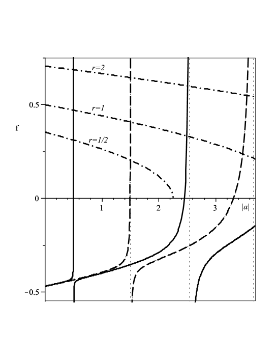
A few qualitative results can be obtained with the aid of a plot of the functions $f$ and $g$ on the same grid. Figure 2 shows the behaviour of $f$ against $|a|$ for two different values of $\sqrt{\omega}L$, and $g$   for three different values of $r$. The eigenenergies are determined by the intersections of the curves defined by $f$ with the square-root function defined by $g$ ($0<g<\sqrt{r}/2$). Without ever solving the quantization condition one is now apt to draw some conclusions about the localized oscillator. It is instructive to note that this process for determining the spectrum for the localized oscillator looks similar to that one for the square potential. Notwithstanding, the zeros and poles of $f$ do not occur at regular intervals as they do for $\tan\left(x\right)$ and $\cot\left(x\right)$.

Seen as a function of $|a|$, $f$ presents branches of monotonically increasing curves limited by vertical asymptotes due to the zeros of $M\left(a/2+1/4,1/2,z_{L}^{2}/2\right)$ and $M\left(a/2+3/4,3/2,z_{L}^{2}/2\right)$. For large $\sqrt{\omega}L$ and small $|a|$, the abscissae of those asymptotes become approximately $n+1/2$, where $n$ is a nonnegative integer, and so do the zeros of $f$.

Since the confluent hypergeometric function goes to $1$ as $z_{L}\rightarrow 0$, one has that $f\rightarrow|a|$ for even parity solutions and $f\rightarrow-\infty$ for odd ones as $\sqrt{\omega}L\rightarrow 0$. Then, because the square-root function vanishes for $|a|=r\left(z_{L}/2\right)^{2}$ just one eigenenergy, that one associated with an even parity eigenfunction with $|a|\simeq 0$, is allowed.

The number of possible bound states grows with $r\left(z_{L}/2\right)^{2}$ but it is restricted by the value of $|a|$ which makes the square-root function vanish. Therefore, the bound-states solutions constitute a finite set of solutions if the potential parameters are finite.

The spectrum consists of energy levels associated with eigenfunctions of alternate parities. The number of allowed bound states grows as the potential parameters increase and there is at least one solution, no matter how small  the parameters are. All the eigenenergies, in the sense of $|a|$, tend asymptotically to the values $n+1/2$ as $\sqrt{\omega}L\rightarrow\infty$ ($n=0,1,2,3,\ldots$). The energy levels tend to higher energies as the parameter $r$ increases. As a function of $\sqrt{\omega}L$, the energy level is a monotonous increasing function for $r\leq 1$ but enclosing the oscillator with vertical walls ($r>1$) makes the energy level to reach a maximum for some value of $\sqrt{\omega}L$.

4 Approximate analytical calculations

Asymptotic representations and limiting forms for the confluent hypergeometric function allow us to obtain approximate analytical results for the special cases of low-lying states and high-lying states.

The asymptotic expression which determines $M\left(a,b,z\right)$ for $a\rightarrow-\infty$ reads [25]

$$M(a,b,z)=\Gamma(b)e^{z/2}\left(\frac{1}{2}bz-az\right)^{\frac{1}{4}-\frac{b}{2}}\pi^{-1/2}$$

$$\times\cos\left[\sqrt{2bz-4az}+\left(\frac{1}{4}-\frac{b}{2}\right)\pi\right]\left[1+\mathcal{O}\left(|b/2-a|^{-1/2}\right)\right],\quad\textrm{for }z\in\mathbb{R}$$ (33)

Since $\Gamma\left(3/2\right)=\Gamma\left(1/2\right)/2$, it follows that the quantization condition expressed by (28) takes the form

$$kL-\frac{z_{L}^{2}}{2}\simeq\left\{\begin{array}[]{c}\left(\sqrt{|a|}z_{L}\right)\tan\left(\sqrt{|a|}z_{L}\right)\\ \\ -\left(\sqrt{|a|}z_{L}\right)\cot\left(\sqrt{|a|}z_{L}\right)\end{array}\begin{array}[]{c}\textrm{for even parity solutions}\\ \\ \textrm{for odd parity solutions}\end{array}\right.$$ (34)

A further simplification occurs for $V(L)-V(0)<<|E|<<|V(0)|$, when $kL>>z_{L}^{2}/2$:

$$kL\simeq\left\{\begin{array}[]{c}\left(\sqrt{|a|}z_{L}\right)\tan\left(\sqrt{|a|}z_{L}\right)\\ \\ -\left(\sqrt{|a|}z_{L}\right)\cot\left(\sqrt{|a|}z_{L}\right)\end{array}\begin{array}[]{c}\textrm{for even parity solutions}\\ \\ \textrm{for odd parity solutions}\end{array}\right.$$ (35)

In this case the eigenfunction inside the well turns into

$$\psi\left(x\right)\simeq c_{e}\,\cos\left(\sqrt{|a|}\alpha x\right)+\frac{c_{o}}{\sqrt{|a|}}\,\sin\left(\sqrt{|a|}\alpha x\right)$$ (36)

Here we considered high-lying states in a harmonic potential extending far down ($r>>1$) and got the solutions for a square well potential. It means that we may neglect any effects associated with the bottom of $V(x)$ as far as high-lying states are concerned. It is instructive to note that the condition $V(L)-V(0)<<|V(0)|$ makes the bottom of the potential look flat.

For small $z$, the hypergeometric function $M\left(a,b,z\right)$ goes like

$$M\left(a,b,z\right)=1+\frac{a}{b}\,z+\frac{a\left(a+1\right)}{2b\left(b+1\right)}\,z^{2}+\ldots$$ (37)

Thus, the quantization condition for $z_{L}<<1$ turns into

$$\begin{array}[]{c}|a|+\left(|a|^{2}-\frac{r}{4}\right)z_{L}^{2}\simeq 0\\ \\ \,1+\frac{|a|}{3}\,z_{L}^{2}\simeq 0\end{array}\begin{array}[]{c}\textrm{for even parity solutions}\\ \\ \\ \textrm{for odd parity solutions}\end{array}$$ (38)

Hence, just one root is allowed: $|a|\simeq 0$ for the even parity solution. This quasi-null eigenenergy solution and its very delocalized eigenfunction are valid for $\sqrt{\omega}L<<\sqrt{\hslash/m}$ when $V(0)\simeq 0$. In this case the potential looks like a little ripple, a shallow well.

On the other hand, for large values of $|z|$ one has [25]

$$\frac{M\left(a,b,z\right)}{\Gamma\left(b\right)}\simeq\frac{e^{z}\,z^{a-b}}{\Gamma\left(a\right)}\,,\quad\textrm{for Re }z>0$$ (39)

In conjunction with the identity $\Gamma\left(z+1\right)=z\,\Gamma\left(z\right)$ and with the fact that $\Gamma\left(z\right)$ has simple poles at $z=-n$   with $n=0,1,2,3,\ldots$, the insertion of (39) into (29) furnishes

$$f\simeq\left\{\begin{array}[]{c}-1/2\\ \\ {\textrm{undefined}}\end{array}\begin{array}[]{c}\textrm{for }|a|\neq n+1/2\\ \\ \textrm{for }|a|=n+1/2\end{array}\right.$$ (40)

for both even and odd parity solutions. The singular behaviour of $f$ when $|a|=n+1/2$ is the reason that it undergoes infinite discontinuities at those values of $|a|$, as can be grasped from Figure 2. It follows that, for sufficiently large $z_{L}$, the square-root function can be expressed by

$$g\simeq\frac{\sqrt{r}}{2}$$ (41)

and the values

$$|a|\simeq\left\{\begin{array}[]{c}2n+1/2\\ \\ 2n+3/2\end{array}\begin{array}[]{c}\textrm{for even parity solutions}\\ \\ \textrm{for odd parity solutions}\end{array}\right.$$ (42)

fulfill the quantization condition. Eq. (42) represents a convenient approximation as far as one considers the lowest values of $|a|$. As a matter of fact, the intersections of the functions $f$ and $g$ occur just slightly below the abscissae of the vertical asymptotes of $f$. Indeed, a better approximation is obtained as $r$ grows. Nevertheless, for all the values of $r$, the agreement improves as $z_{L}$ gets larger. In this approximation, $M\left(a,b,z\right)$ reduces to a polynomial of degree $n$ in $z$ when $a=-n$. In particular, for $b=1/2$ and $b=3/2$ one has [25]

$$H_{2n}\left(x\right) = \left(-1\right)^{n}\frac{\left(2n\right)!}{n!}M\left(-n,\frac{1}{2},x^{2}\right)$$

$$H_{2n+1}\left(x\right) = \left(-1\right)^{n}\frac{\left(2n+1\right)!}{n!}\,2x\,M\left(-n,\frac{3}{2},x^{2}\right)$$ (43)

where $H_{n}\left(x\right)$ is the Hermite polynomial. Therefore, for $\sqrt{\omega}L>>\sqrt{\hslash/m}$ one gets the condensed form

$$E_{n}\simeq V\left(0\right)+\left(n+\frac{1}{2}\right)\,\hslash\omega,\quad\psi_{n}\left(x\right)\simeq N_{n}\,e^{-\alpha^{2}x^{2}/4}H_{n}\left(\frac{\alpha x}{\sqrt{2}}\right)$$ (44)

where $N_{n}$ is a normalization factor. The approximate results for $\sqrt{\omega}L>>\sqrt{\hslash/m}$ are expected to be exact in the limit $L\rightarrow\infty$ when the potential goes over to the full-space harmonic oscillator. It is comforting to note that the particular values of $|a|$ obtained from the quantization condition are the same as those which make the eigenfunction normalizable on the interval $\left(-\infty,+\infty\right)$. The harmonic oscillator approximation for $\sqrt{\omega}L$ finite, though, is only reasonable for the low-lying states, i.e. for energy levels so near of the bottom of the potential that edge effects can be neglected.

5 Exact results

The only remaining question is how to determinate exact results. With the eigenfunctions on the whole line expressed by (18) and (19), the problem resumes to find the eigenenergies. Although the quantization condition has no closed form solutions in terms of simpler functions, the numerical computation of the allowed values of $|a|$ can be done easily with a root-finding procedure of a symbolic algebra program.

Figure 3 is a plot of the first low-lying energy levels, in the sense of $|a|$, as a function of $\sqrt{\omega}L$. The bound-states solutions of the localized and unconfined oscillator constitute a finite set of solutions. The number of allowed bound states increases with $\sqrt{\omega}L$ and there is at least one solution, no matter how small is $\sqrt{\omega}L$. All the eigenvalues tend asymptotically to the values $n+1/2$ as $\sqrt{\omega}L\rightarrow\infty$ ($n=0,1,2,3,\ldots$). The energy levels tend toward higher energies as the parameter $r$ increases, as can also be seen in Figure 2. As a function of $\sqrt{\omega}L$, the energy level is a monotonous increasing function for $r\leq 1$ but enclosing the oscillator with a square well potential ($r>1$) makes the energy level reach a maximum for some value of $\sqrt{\omega}L$.

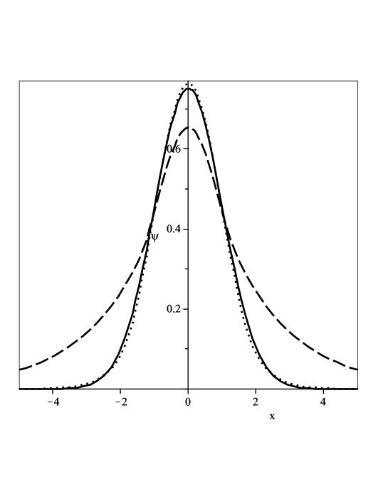
Figure 4 shows the results for the ground-state eigenfunction against $x$ for $\sqrt{\omega}L=3/2\sqrt{\hslash/m}$ and $L$ equal to a Compton wavelength. Included for comparison is the ground-state eigenfunction for the full harmonic oscillator. The normalization $\int_{-\infty}^{+\infty}dx\,|\psi|^{2}=1$ was done numerically. The eigenfunctions for $r=2$ ($|a|\simeq 0.520$) and $r=1/2$ ($|a|\simeq 0.416$) differ from that for the full harmonic oscillator. The approximation does better for $r=2$, as it does for the eigenvalue. In fact, the agreement is not bad even though we have used $\sqrt{\omega}L\sim\sqrt{\hslash/m}$. Just as expected from the above qualitative analysis, a more successful agreement for all the values of $r$ should be obtained for $\sqrt{\omega}L>>\sqrt{\hslash/m}$.

6 Conclusions

We have assessed the bound-state solutions of the Schrödinger equation with a localized and unconfined harmonic potential well. We have derived the energy eigenvalue equation and shown explicitly the eigenfunctions. We have discussed the structure of the solutions of the eigenvalue equation. The structure of the eigenfunctions has also been presented. The satisfactory completion of this task has been alleviated by the use of graphical methods and tabulated properties of the confluent hypergeometric functions. Finally, the exact results have been presented.

As mentioned in the introduction of this work, the three-parameter oscillator potential presents a richness of physics which might be relevant for calculations in different fields of solid state physics, particularly in electronics and computer components. Furthermore, it renders a sharp contrast to the oscillator confined by infinite walls [4]-[8].

Acknowledgments

This work was supported in part by means of funds provided by CAPES and CNPq.

(a) $r>1$

(b) $r=1$

(c) $0<r<1$

(d) $r<0$

Figure 1: Profiles for $V(x)$.

(a) $\sqrt{\omega}L=2\sqrt{\hslash/m}$

(b) $\sqrt{\omega}L=3\sqrt{\hslash/m}$

Figure 2: Graphical representation for $f$ as a function of $|a|$. The continuous line for even parity solutions, the dashed line for odd ones, and the dotted line for the asymptote. The dashed-dotted line stands for the square-root function.

Figure 3: $|a|$ for the first three energy levels as a function of $\sqrt{\omega}L$ (in units of $\sqrt{\hslash/m}$) for three representative values of $r$. The dotted parabola stands for the threshold for the existence of bound states given by $|V(0)|/\hslash\omega$.

Figure 4: Eigenfunction for the ground state as a function of $x$ for $\sqrt{\omega}L=3/2\sqrt{\hslash/m}$ and $L$ equal to the Compton wavelength. The continuous line for the full harmonic oscillator, the dashed line for $r=1/2$ and the dotted line for $r=2$.

References

- [1] A. Michels, J. de Boer and A. Bijl, Physica 4, 981 (1937).
- [2] A. Sommerfeld and H. Hartmann, Ann. Phys. (Lpz.) 37, 333 (1940).
- [3] S. Chandrasekhar, Astrophys. J. 97, 263 (1943).
- [4] F. C. Auluck and D. S. Kothari, Proc. Camb. Phil. Soc. 41, 175 (1945).
- [5] J. S. Baijal and K. K. Singh, Prog. Theor. Phys. 14, 214 (1955).
- [6] T. E. Hull and R. S. Julius, Can. J. Phys. 34, 914 (1956).
- [7] P. Dean, Proc. Camb. Phil. Soc. 62, 277 (1966).
- [8] R. Vawter, Phys. Rev. A 174, 749 (1968).
- [9] W. N. Mei and Y. C. Lee, J. Phys. A 16, 1623 (1983).
- [10] H. E. Montgomery, Jr., N. A. Aquino and K. D. Sen, Int. J. Quantum Chem. 107, 798 (2007).
- [11] S. M. Al-Jaber, Int. J. Theor. Phys. 47, 1853 (2008).
- [12] H. E. Montgomery, Jr., G. Campoy and N. A. Aquino, math-ph/0803.4029.
- [13] R. de L. Kronig and W. G. Penney, Proc. R. Soc. London, ser. A, 130, 499 (1930).
- [14] L. L. Chanz and L. Esaki, Phys. Today 45, 36 (1992).
- [15] C. W. J. Beenakker and A. A. M. Staring, Phys. Rev. B 46, 9667 (1992).
- [16] N. Maitra and E. J. Heller, Phys. Rev. Lett. 78, 3035 (1997).
- [17] C. V. Reddy et. al., App. Phys. Lett. 77, 1167 (2000).
- [18] A. Chandra e L. F. Eastman, J. Appl. Phys. 53, 9165 (1982).
- [19] S. L. Ban, J. E. Hasbun and X. X. Liang, Journal of Luminescence 87, 369 (2000).
- [20] W. W.Lui and M. Fukuma, J. Appl. Phys. 60, 1555 (1986).
- [21] Y.Ma et al., IEEE Trans. Electron Devices 47, 1764 (2000).
- [22] N. A. Rao and B. A. Kagali, EJTP 5, 169 (2008).
- [23] L. B. Castro and A. S. de Castro, EJTP 7, 155 (2010).
- [24] H. Cruz, A. Hernández-Cabrera and A. Muñoz, Semicond. Sci. Technol. 6, 218 (1991).
- [25] M. Abramowitz and I. A. Stegun, Handbook of Mathematical Functions, Dover, Toronto, 1965.