Growth and anisotropy of ionization fronts near high redshift quasars in the MassiveBlack simulation

Abstract

We use radiative transfer to study the growth of ionized regions around the brightest, $z=8$ quasars in a large cosmological hydrodynamic simulation that includes black hole growth and feedback (the MassiveBlack simulation). We find that in the presence of the quasars the comoving HII bubble radii reach $10\,\mathrm{Mpc/h}$ after 20 Myear while with the stellar component alone the HII bubbles are smaller by at least an order of magnitude. Our calculations show that several features are not captured within an analytic growth model of Stromgren spheres. The X-ray photons from hard quasar spectra drive a smooth transition from fully neutral to partially neutral in the ionization front. However the transition from partially neutral to fully ionized is significantly more complex. We measure the distance to the edge of bubbles as a function of angle and use the standard deviation of these distances as a diagnostic of the anisotropy of ionized regions. We find that the overlapping of nearby ionized regions from clustered halos not only increases the anisotropy, but also is the main mechanism which allows the outer radius to grow. We therefore predict that quasar ionized bubbles at this early stage in the reionization process should be both significantly larger and more irregularly shaped than bubbles around star forming galaxies. Before the star formation rate increases and the Universe fully reionizes, quasar bubbles will form the most striking and recognizable features in 21cm maps.

1 Introduction

The current consensus is that the contribution to the global ionizing budget from quasars during the Epoch of Reionization (EoR) is small compared to that from early stars and galaxies (see, eg, Loeb, 2009; Giroux & Shapiro, 1996; Trac & Gnedin, 2011). The EoR began as the population III stars and primordial galaxies ionized their most immediate vicinity, as studied by Thomas & Zaroubi (2008); Chen & Miralda-Escudé (2008); Venkatesan & Benson (2011). On the other hand, the characteristic proper radius of ionizing bubbles at the end of EoR is constrained to be on the order of $10\,\mathrm{Mpc/h}$ (Maselli et al., 2007; Alvarez & Abel, 2007; Wyithe & Loeb, 2004), and the quasar contribution is limited to be less than 14% (Srbinovsky & Wyithe, 2007) of the total. Even though the contribution to global reionization by quasars is constrained in this way, bright quasars may still leave a signature on the growth of individual ionized regions. Several authors have investigated this signature in mock 21cm emission spectra taken from simulations of isolated quasars (Datta et al., 2012; Majumdar et al., 2011; Alvarez et al., 2010; Datta et al., 2008; Geil & Wyithe, 2008) at redshift $z\sim 8$. In observations, an object recently reported by Mortlock et al. (2011), ULAS J1120+0641, has a luminosity of $6.3\times 10^{13}L_{\odot}$ at $z\sim 7$ and a proper near-zone radius of less than $2\,\mathrm{Mpc/h}$. The near-zone radius is consistent with the possibility of bright quasar driven growth in a near neutral intergalactic medium background (Bolton et al., 2011).

In this paper we study the growth of the ionization front of bright quasars in an almost neutral cosmological context. The quasars and their surrounding medium are selected from a large hydrodynamic simulation (the MassiveBlack simulation, introduced in Di Matteo et al., 2012), and then post-processed with a radiative transfer code. This allows us to simulate 8 rare quasars using reasonable computing resources. Our focus is on the evolution and properties of the largest individual ionized bubbles, the sources that produce them, and the relationship between the two. Because the simulation forms quasars and star forming galaxies ab initio, we are able to make use of the luminosity and positions of the radiation sources that the simulation produces, rather than setting them in by hand. However we do not deal with the full reionization of the volume of the simulation, which would require following the evolution of the entire density and ionization field from high redshifts down to at least $z=6$. Instead we restrict ourselves to the growth of ionized regions around an early period in this process (at $z=8$), where the photon path lengths are still smaller than the computational sub-volumes we analyze. We leave the study of the full reionization of the volume to future work.

2 Hydrodynamic simulation and density field

The SPH output we use is from the MassiveBlack simulation (see Di Matteo et al., 2012; DeGraf et al., 2012; Khandai et al., 2012, for further details), which was run with a $\Lambda\rm CDM$ cosmology with parameters $(\Omega_{\Lambda},\Omega_{M},\Omega_{b},h,\sigma_{8})=(0.74,0.26,0.044,0.72,0.8)$. A total number of $2\times 3200^{3}$ gas and dark matter particles were followed in a box of $0.75\,\mathrm{Gpc^{3}}$ from redshift $z=159$ to redshift $z=4.75$. This simulation is by far the largest cosmological hydrodynamics simulation run with the P-GADGET program. This run not only contains gravity and hydrodynamics but also the extra physics (sub-grid modeling) for star formation (Springel & Hernquist, 2003), black holes and associated feedback processes.

The basics aspects of the black hole accretion and feedback model (Di Matteo et al., 2008) consist of representing black holes by collisionless particles that grow in mass (from an initial seed black hole) by accretion of gas in their environments. The accretion rate is given by

$$\dot{M}=\min(M_{\rm Bondi},M_{\rm Edd})\,,$$ (1)

and

$$\dot{M}_{\rm Bondi}=\frac{4\pi G^{2}M_{BH}^{2}\rho}{(c_{s}^{2}+v^{2})^{3/2}},$$ (2)

where $\rho$ and $c_{s}$ are the density and sound speed of the ISM gas respectively, and $v$ is the velocity of the black hole relative to the gas, and $\dot{M}_{\rm Edd}=L_{\rm Edd}/(\eta c^{2})$, where $L_{\rm Edd}=1.26\times 10^{38}\,\mathrm{ergs^{-1}}$, is the Eddington Luminosity. At the high redshift and high halo masses we are carrying out the analysis here, black holes are growing at their Eddington rates (DeGraf et al., 2012) making any detail of the sub-grid models for black holes virtually irrelevant.

For the black hole feedback, a fraction of the radiative energy released by the accretion of material is assumed to couple thermally to nearby gas and influence its motion and thermodynamic state. The radiated luminosity, $L_{\rm r}$, from the black hole is related to accretion rate, $\dot{M}_{\rm BH}$, as

$${{L_{\rm bol}}=\eta{\dot{M}_{\rm BH}c^{2}}},$$ (3)

where we take the standard mean value $\eta=0.1$. Some coupling between the liberated luminosity and the surrounding gas is expected: in the simulation 5% of the luminosity is isotropically deposited as thermal energy in the local black hole kernel, providing some form of feedback energy.

With our simulations the activity of quasars is directly derived from the accretion history of rapidly growing super-massive black holes, and their fueling is driven from the large scales and occurs through high density cold flows along the cosmic filaments (Di Matteo et al., 2012).

The luminosity of the stars and galaxies can be derived from the star formation rate history which is provided by the multiphase star formation model in the simulation that depends on a single free parameter, $t_{\star}$ the global star formation timescale (Springel & Hernquist, 2003). The multiphase star formation model also provides a mechanism to remove the self-shielded interstellar medium (ISM) from the matter density field, leaving only the intergalactic medium (IGM) density for the radiative transfer simulation.

In the multiphase star formation model, a dense gas particle is divided into a non-star forming IGM component and a star forming ISM component:

$$m=\begin{cases}m_{\rm IGM}+m_{\rm ISM}=(1-x)m+xm,&\mbox{if }\rho>\rho_{\rm th},\\ m_{\rm IGM},&\mbox{if }\rho\leq\rho_{\rm th},\\ \end{cases}$$ (4)

where $x$ is the mass fraction of the ISM component. The threshold density $\rho_{\rm th}$ is determined from the global star formation time scale $t_{\star}$, as described in Springel & Hernquist (2003). The IGM component of gas particles forms a hot ambient medium and occupies the entire volume of the particle. The ISM component of gas particles condenses into cold star-forming clouds which are self-shielded from cosmic radiative transfer, except that they may host stellar radiative sources. As a result we excise them from the matter density field when performing the ray tracing calculation. By doing this we also assume that their small cross-section would not have affected ray tracing for the rest of the gas. The ISM fraction, $x$, is an increasing function of the mean density of the gas particle, effectively removing the densest particles from the density field in a manner similar to the threshold method used to calculate the clumping factor by Pawlik et al. (2009), and, the removal of the cold high density gas in the X-ray emission calculation by Croft et al. (2001).

We also note that in MassiveBlack the mean baryon density (IGM + ISM) around quasar sources can be as high as $60\,\mathrm{cm^{-3}}$. Were the ISM not excised from the ray tracing, the high mean density would shield off the radiation and prevent the growth of any cosmic scale ionized regions.

3 Selection of Quasars

We use the quasars and density field of the $z=8$ snapshot of MassiveBlack in this study. There are two reasons for this choice:

• The EoR in MassiveBlack is modeled by a uniform UV background radiation field that is introduced near the end of the EoR ($z=6$) in the optically thin approximation (see e.g. Bolton & Haehnelt, 2007). By choosing an earlier redshift we do not contaminate the ionization fronts with this global radiation field.

• Extremely bright quasar sources at high redshifts are rare objects. Limited by the $0.75\,\mathrm{Gpc^{3}}$ volume of MassiveBlack, we cannot find many bright quasar systems at a much higher redshift than $z=8$.

We select a quasar system based on halo mass, taking the 10 most massive halos, numbered from 0 to 9. We note that in general larger halos host brighter quasars unless (i) the quasar system is turned off by feedback, or (ii) the quasar system has not yet grown its black hole mass significantly. 8 unique hosting sub-volumes ($50\,\mathrm{Mpc/h}$ per side) are identified, which we refer as sub-volume 0 to 7 throughout the rest of the paper: Three of the halos (halo number 0, 3 and 5 in Table 1) are located at spatial locations within sub-volume 0.

#H	#V	$M_{\rm HALO}$	$M_{\rm BH}$	Total		Center
				QSO	STR	QSO	STR
0	0	148.35	74.6	8.35	3.38	7.24	0.94
1	1	77.9	49.6	4.97	3.45	4.43	0.79
2	2	75.5	34.7	2.06	3.93	1.39	0.45
3	0	84.9	7.3	8.35	3.71	0.49	0.22
4	3	60.1	119.0	8.18	2.72	7.76	0.54
5	0	67.1	16.0	8.35	3.71	0.56	0.21
6	4	70.8	5.5	0.50	2.72	0.06	0.16
7	5	65.6	13.2	0.95	1.98	0.69	0.30
8	6	66.6	6.4	1.29	3.82	0.20	0.21
9	7	64.9	7.2	0.38	2.22	0.15	0.15

Table 1: UV Flux of Sub-volumes. The first column #H (0 - 9) identifies the ten most massive halos. The second column #V (0 - 7) identifies the eight unique sub-volumes that contain the halos. The halo mass ($M_{\rm HALO}$) is in units of $10^{10}\,\mathrm{M_{\odot}h^{-1}}$. The blackhole mass ($M_{\rm BH}$) is in units of $10^{6}\,\mathrm{M_{\odot}h^{-1}}$. The flux is in units of $10^{55}\,\mathrm{sec^{-1}}$. Halos 0, 3, and 5 are clustered and belong to the same sub-volume 0. See Appendix A for the definition of the spectra.

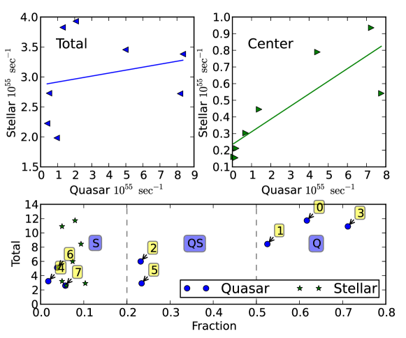
Figure 1: Central and total ionizing photon flux. The left panel compares the total UV photon flux of the stars and the quasars within the sub-volumes. The right panel compares the UV photon flux from the sources within $1\,\mathrm{Mpc/h}$ of the center. The lines represent the linear regression of the data. In the bottom panel the central photon flux of the quasar sources and the central photon flux of the stellar sources as a fraction of the total flux are shown. It is interesting to observe that the central stellar photon flux is always a small fraction of the total flux yet the central quasar can contribute a significant fraction of the total. See Appendix A for the definition of the spectra.

Next, we compute the ionizing photon flux due to the quasars and star formation occurring in each of the sub-volumes. The details of the assignment are described in Appendix A. In addition to the full volume flux, we also define a Central Source Flux, which is the flux of sources within the $1\,\mathrm{Mpc/h}$ radius of the center of the sub-volume. The sources in the center are associated with the ionized bubble of the central halo. The ionizing photon flux of the sub-volumes is summarized in Table 1 and Figure 1.

There is an expected correlation between the central quasar and central stellar flux. Based on the ratio of the central flux to total ionizing flux within the sub-volume, as well as the composition (quasar or stellar) of the central flux, we divide the sub-volumes into three groups:

• Quasar (Q) : The central quasar dominates the entire sub-volume.

• Sub-dominant Quasar (QS) : The central quasar dominates the central flux, but is not a significant fraction of the total flux of sources in the sub-volume.

• Stellar (S): The quasar flux in the central sources is smaller than the sum of stellar flux, and the entire central flux is small compared to the ionizing flux of the entire box. We note there can be two possible distributions of sources within the box: one being the presence of another major source that is not near the center of the sub-volume; the other being ionizing sources that are rather more uniformly distributed throughout the sub-volume. In our sub-volumes, the latter is more often to the case.

4 Analytic Growth of Stromgren Spheres

The growth of Stromgren spheres in a clumpy cosmological environment can be analytically modeled using (Cen & Haiman, 2000),

$$\frac{dR_{t}^{3}}{dt}=3H(z)R_{t}^{3}+\frac{3\dot{N}_{\rm ph}}{4\pi\left\langle n_{\rm H}\right\rangle}-C_{\rm H}\left\langle n_{\rm H}\right\rangle\alpha_{\rm B}R_{t}^{3},$$ (5)

where the first term represents the Hubble expansion, and can be neglected in this context. The solution is straightforward (eg, Shapiro & Giroux, 1987)

$$R_{t} = R_{s}\left(1-\exp\left(-\frac{t}{t_{s}}\right)\right)^{-\nicefrac{{1}}{{3}}}\approx R_{s}\left(\frac{t}{t_{s}}\right)^{\nicefrac{{1}}{{3}}}$$

$$t_{s} = \left(C_{\rm H}\left\langle n_{\rm H}\right\rangle\alpha_{\rm B}\right)^{-1}$$ (6)

$$R_{s} = \left(\frac{3\dot{N}_{\rm ph}}{4\pi C_{\rm H}\left\langle n_{\rm H}\right\rangle^{2}\alpha_{\rm B}}\right)^{\nicefrac{{1}}{{3}}}.$$

We will use this analytic solution to compare to our numerical results. The IGM clumping factor $C_{\rm H}$ is calculated using a method appropriate for an SPH simulation, described by Pawlik et al. (2009),

$$C_{\rm H}=\frac{\sum\rho_{i}^{2}h_{i}^{3}}{\left\langle\rho\right\rangle^{2}\sum h_{i}^{3}},$$ (7)

where $h_{i}$ is the SPH smoothing length, and $\rho_{i}$ is the IGM density. The clumping factor in the entire sub-volumes has a value of $C_{H}\sim 4$, giving a recombination time about $t_{S}\sim 100\,\mathrm{Myear}\gg t_{Q}$. However we note the clumping factor can go up to $\sim 20$ within $1\,\mathrm{Mpc/h}$ radius from the center of the sub-volume, reducing $t_{S}$ to $\sim 20\,\mathrm{Myear}$.

For the source flux, we make the simplest approximation, summing the flux of all sources with in the sub-volume to obtain one effective $\dot{N}_{\rm ph}$. We also assume that the volume consists of pure hydrogen (i.e. no helium, $X_{\rm H}=1$) in the calculation of the analytic model. The Case B recombination rate $\alpha_{\rm B}$ is taken from Hui & Gnedin (1997), in consistency with the recombination rate table used in the radiative transfer simulation.

5 Radiative Transfer Simulation

5.1 Ray-tracing Scheme

For this study we have rewritten the SPHRAY Monte Carlo radiative transfer code (Altay et al., 2008; Croft & Altay, 2008) in C with OpenMP(TM), so that it runs in parallel on shared memory systems (P-SPHRAY). We have also eliminated the on-the-spot approximation of recombination, so that instead recombination rays are emitted when the recombination photon deposit at a spot exceeds a threshold, as done in the code CRASH (Maselli et al., 2003). The parallel version allows us to trace many rays at the same time on several CPUs within a single time step, achieving a near-linear speed up with a small number (10 $\sim$ 30) of CPUs. Monochromatic rays are sampled from frequency space according to the source spectrum. Hydrogen and Helium ionization and recombination are both traced. The tabulated atomic reaction rates of Hui & Gnedin (1997) taken from the serial version SPHRAY are used.

As a new addition to the code we model the secondary ionization of high energy photons using a fit to the Monte Carlo simulation results of Furlanetto & Stoever (2010); Shull & van Steenberg (1985). These fast non-thermal-equilibrium electrons produced from high energy ionization photons (e.g., X-ray photons) may collide and secondarily ionize more neutral atoms, increasing the ionizing efficiency of the quasar sources by allowing one high energy photon to ionize tens of neutral atoms. On the other hand, our current post-processing approach is incapable of modeling the heating from the residual energy of the ionizing photons, for the thermal evolution (hydro) is decoupled from radiative transfer. We note that the local heating of ionizing photons can be thought of as part of the local thermal coupling between the liberated luminosity and the surrounding environment described in Section 2. The long range heating of the harder photons is not directly modeled.

5.2 Parametrization of the Ionized Bubble

For this study, we are more interested in the ionized bubbles located at the centers of sub-volumes, because they are associated with the main halos in the sub-volumes. We will call these central ionized bubbles the central ionized regions (CIR).

When quantifying the size of a CIR we measure the spherically averaged fraction of a species, $x$ using (we show the example of HII regions, similar definitions hold for other species):

$$x_{\rm HI}(r)=\frac{\int\delta(r^{\prime}-r)x_{\rm HI}\rho dV}{\int\delta(r^{\prime}-r)\rho dV}\doteq\frac{\sum_{\rm shell}x_{\mathrm{HI},i}m_{i}}{\sum_{\rm shell}m_{i}}.$$ (8)

Here the sums are carried out by binning SPH particles (index $i$) in shells. Particles are assigned as a whole to shells by their center position rather than being integrated over the SPH kernel with in the shell. We define the averaged CIR radius at a given threshold $x^{*}$ to be the first crossing of $x(r)$ with $x^{*}$, or

$$\hat{R}_{S}(x)=\inf\{r|x_{\rm HI}(r)=x^{*}\}.$$ (9)

The first crossing corresponds to the edge of the CIR, and later crossings indicate the edges of the nearby ionized regions. The motivation for this definition comes from its similarity to that used to quantify ionized regions seen in quasar absorption line spectra, the Ly$\alpha$ absorption Near-Zone radius $R_{NZ}$ by Fan et al. (2006). In practice, we take as $\hat{R}_{S}$ the average of the two nearest bins $r_{L}$ and $r_{R}$ which satisfy $[x_{\rm HI}(r_{L})-x][x_{\rm HI}(r_{R})-x]<0$.

The spherically averaged radius $\hat{R}_{S}$ is a simple quantity to use in comparisons but the angular variations in the properties of the CIR are completely lost. To quantify the angular dependency, we bin the SPH particles into angular cones and calculate the averaged fraction within the cones,

$$x_{\rm HI}(r,\theta,\phi)\doteq\frac{\sum_{\rm cone,shell}x_{\mathrm{HI},i}m_{i}}{\sum_{\rm cone,shell}m_{i}}.$$ (10)

The angular dependent CIR radius is

$$R_{s}(x,\theta,\phi)=\inf\{r|x_{\rm HI}(r,\theta,\phi)=x^{*}\}.$$ (11)

Note that in general $<R_{s}(x,\theta,\phi)>\neq\hat{R}_{S}$, because averaging and binning do not commute. For measuring $R_{s}(x,\theta,\phi)$, we use $12\times 16^{2}$ cones. We note that increasing to $12\times 32^{2}$ cones does not significantly alter the results.

We measure the anisotropy of the ionized bubble from the variance of $R_{s}$

$$A_{s}(x)=ST{}_{k}[R_{s}(x,\theta_{k},\phi_{k})],$$ (12)

where $ST_{k}$ stands for the standard derivation. We run the simulation with sufficient number of rays so that the typical shot-noise contribution towards $A_{s}$ is negligible, as shown in the next section.

Three different levels of species fraction $x$ are used to define three different levels of CIR fronts in this study:

• Inner front, $x=0.1$ for the neutral fraction, or $x=0.9$ for the ionized fraction;

• Middle front, $x=0.5$ for the neutral fraction;

• Outer front, $x=0.9$ for the neutral fraction, or $x=0.1$ for the ionized fraction.

The Inner front corresponds to the near-ionized edge of the Stromgren sphere, and the Outer front corresponds to the near-neutral edge of the Stromgren sphere. We however note that these choices are for illustrative purposes and they do not have any direct correspondence with threshold values used to detect $21\,\mathrm{cm}$ or Ly$\alpha$ observation signatures.

5.3 Shot-noise and Convergence

One issue which must be addressed in Monte Carlo ray tracing (RT) schemes is the presence of shot-noise and its effect on convergence of results, something particularly important when sampling is also in frequency space (eg, Iliev et al., 2006, comments on CRASH). Shot-noise artificially increases the angular anisotropy $A_{s}$ measure, and so is of direct concern for this study.

We define a shot-noise parameter $\gamma$ to be the ratio between the number of photons in a ray packet, $n_{r}^{0}$ and the number of atoms in an SPH particle $n_{p}^{0}$,

$$\gamma=\frac{n_{r}^{0}}{n_{p}^{0}}.$$ (13)

A small $\gamma$ guarantees that the ionization front cannot advance by more than one particle in one time step. When $\gamma\ll 1$, the ionization front advances slowly and the shot-noise is controlled. One of course still needs to ensure the rays have a sufficient angular resolution to resolve the angular scale used in the calculation of the anisotropy.

In MassiveBlack, a typical SPH gas particle has a mass of $5\times 10^{7}\,\mathrm{M_{\odot}/h}$, equivalent to $n_{p}^{0}=9\times 10^{64}$. For ray tracing with $10^{5}$ steps and $128$ rays per time step, ($1.28\times 10^{7}$ rays), and with the total luminosity listed in Table 1, an average packet contains $n_{r}^{0}=3\times 10^{63}$ photons. The shot-noise parameter is therefore $\gamma=0.03\ll 1$ for our typical runs.

We can also empirically confirm that convergence is reached by increasing the number of rays used in the simulation and showing that the quantity of interest is insensitive to further increases. We perform such a convergence test with 3 runs on sub-volume 4 with (i) $1.3\times 10^{8}$ rays, $\gamma=0.003$, (ii) $1.3\times 10^{7}$ rays, $\gamma=0.03$, and (iii) $1.3\times 10^{6}$ rays, $\gamma=0.3$. We quantify the similarity of the ionization front using the correlation coefficient of $R_{s}(\theta,\phi)$ between runs, shown in Table 2. The higher correlation between the runs with more rays indicates that the simulation has effectively converged. Therefore, for the runs we use $1.3\times 10^{7}$ rays.

Runs	HII Inner	HII Middle	HII Outer
$\gamma=0.003\leavevmode\nobreak\ \mbox{and}\leavevmode\nobreak\ 0.03$	0.96	0.98	0.86
$\gamma=0.03\leavevmode\nobreak\ \mbox{and}\leavevmode\nobreak\ 0.3$	0.74	0.94	0.68

Table 2: Correlation coefficients in convergence test for number of rays. See Equation 13 for definition of $\gamma$. Shown in the table are the correlation coefficient of the center bubble radius $R_{s}(\theta,\phi)$ between different runs.

6 Results and Discussion

6.1 Uniform Density Field

We first test P-SPHRAY with a source in a uniform density field at $z=8$, with H number density $n_{\rm H}=2\times 10^{-4}\,\mathrm{cm^{-3}}$, and uniform temperature $T=10^{4}\,\mathrm{K}$. The hydrogen mass fraction is $X_{\rm H}=0.76$, the cubical box has a side length of $50\,\mathrm{Mpc/h}$, and we evolve the radiation and ionization fractions for a duration of $2\times 10^{7}\,\mathrm{yrs}$. We carry out 3 separate simulations, considering different central source properties for each one as follows: (i) $1.2\times 10^{56}\,\mathrm{sec^{-1}}$ UV; (ii) $1.2\times 10^{56}\,\mathrm{sec^{-1}}$ UV, $0.3\times 10^{55}\,\mathrm{sec^{-1}}$ soft X-Ray, $0.5\times 10^{55}\,\mathrm{sec^{-1}}$ hard X-Ray; (iii) same as (ii), with secondary ionization. The luminosity of the source is motivated by the luminosity of the center sources in sub-volume 0. The growth of the CIR fronts in the simulations are shown as a function of time in Figure 2.

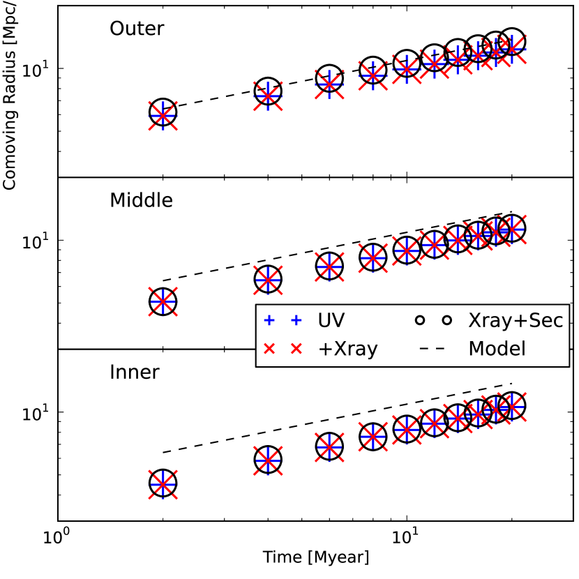
Figure 2: CIR Growth in a Uniform Density Field. The symbols are: (i) cross[+]: UV only; (ii) cross[x]: UV and X-ray (iii) circle: UV and X-ray, with Secondary ionization. The analytic model (dashed lines) neglects Helium and assumes $X_{H}=1.0$.

We show as separate panels the behaviors of the three parts of the ionization front: inner, middle and outer (as defined in Section 5.2).

There are three highlights from the uniform density field simulations: (i) The fronts in general agree well with the analytic model described in 6. (ii) There is a smooth transition from neutral to ionized state at the front, indicated by the $\leavevmode\nobreak\ 1\,\mathrm{Mpc/h}$ difference between the inner front and the outer front. The transition is mostly due to the penetration of harder UV photons. (iii) The effect of X-ray photons and secondary ionization is more evident on growth of the outer front than of the inner and middle fronts. This is because the secondary ionization affects the way the harder photons interact with the matter the most, and harder photons travel further into the neutral region. We note that by adding in the effect of secondary ionization increases the outer radius of ionized bubbles by approximately 10%.

6.2 MassiveBlack: Visualization

We show the CIR bubble of the most extreme Q type and S type sub-volumes (sub-volume number 3 and 4 in Table 1 respectively) in Figure 3. The halo mass of both are similar, $60\times 10^{10}\,\mathrm{M_{\odot}h^{-1}}$ and so are their total star formation rates. However sub-volume 3 has a large ionized HII region associated with the bright active quasar in the center of the sub-volume, whilst in sub-volume 4 the HII region formed merely from stellar sources are small. Note that, even though in a comparable mass halo, the central black hole is much smaller in sub-volume 3 and hence its activity has a negligible impact. This example aims to illustrate how, in the presence of an active early quasar, the ionized bubble is far more extensive than one driven by star formation alone.

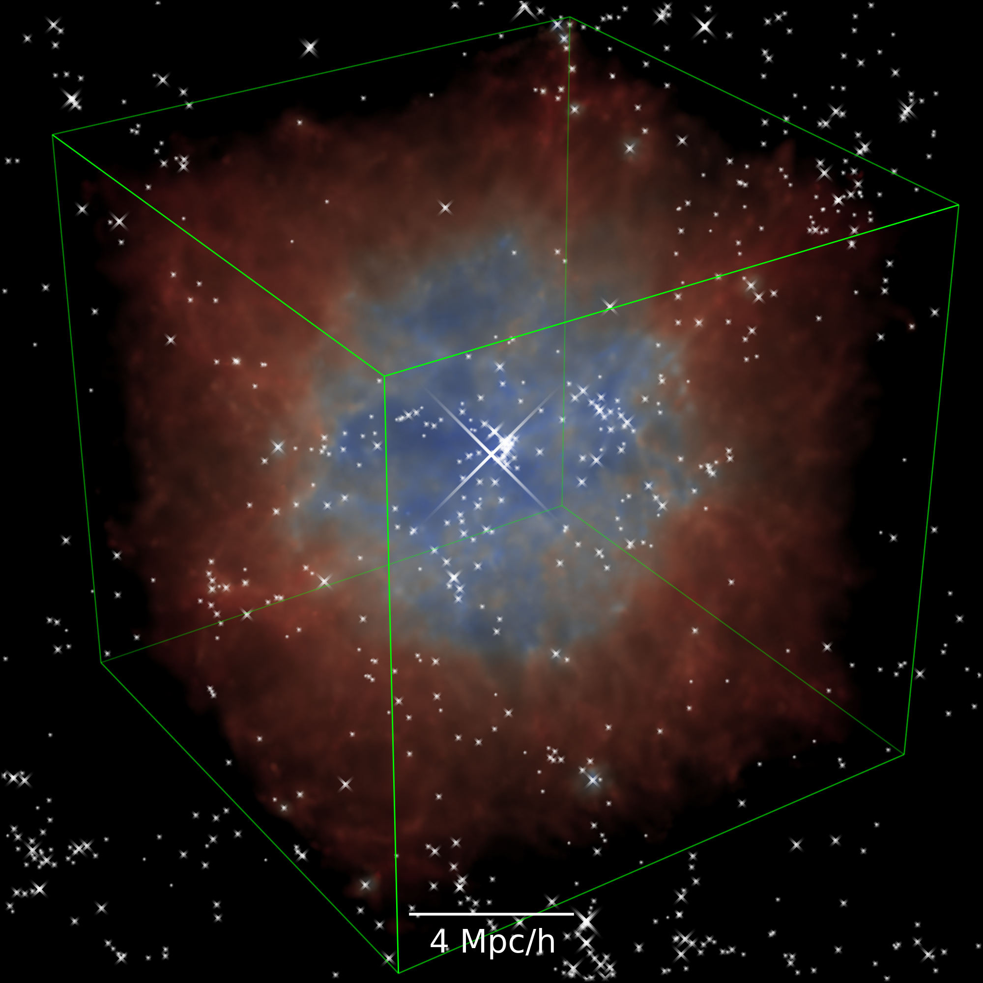
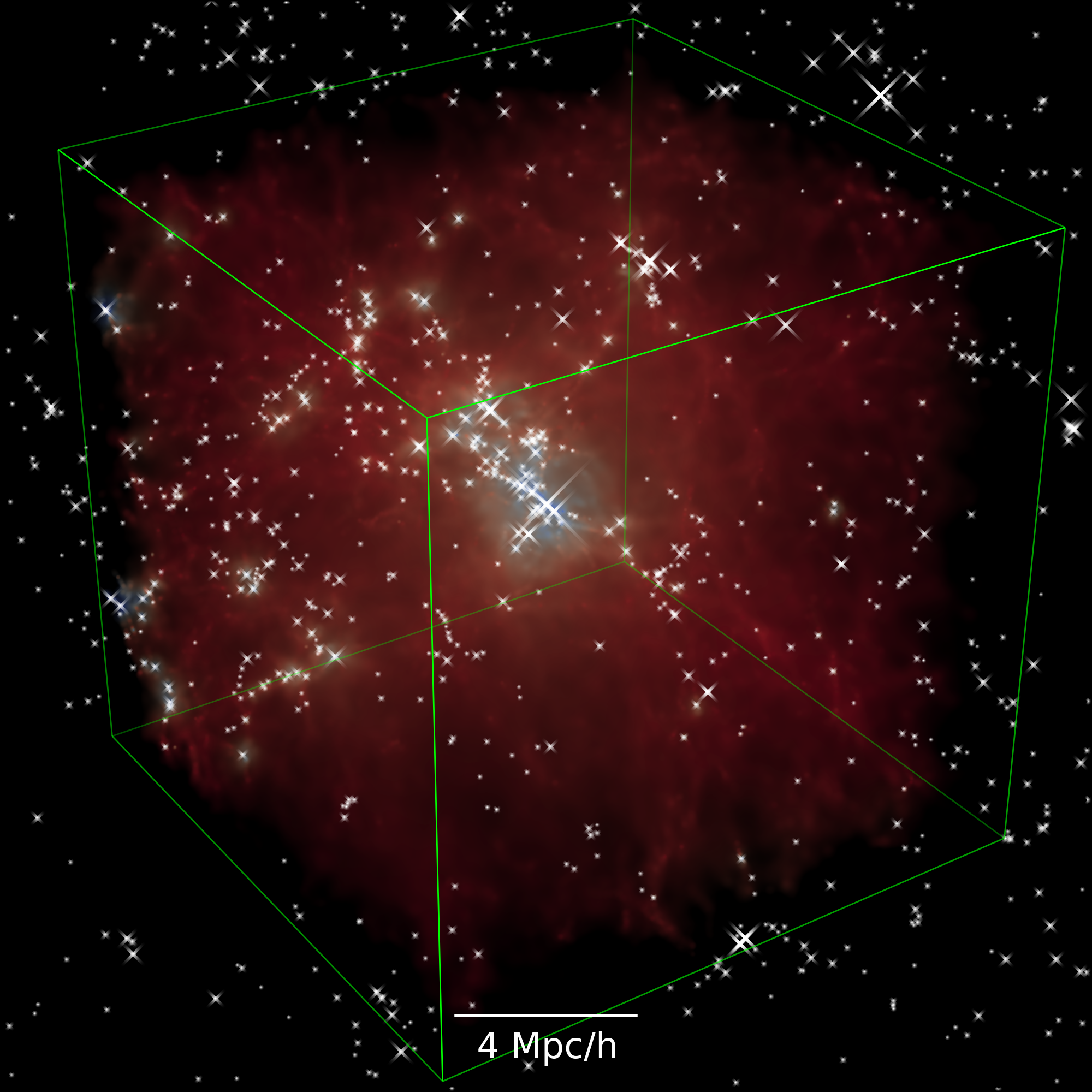
Figure 3: Q (quasar, left) type and S (stellar, right) type ionized bubbles in MassiveBlack. Both panels are of comoving length $15\,\mathrm{Mpc/h}$ per side. A camera is put at about $60\,\mathrm{Mpc/h}$ from the center of the sub-volume and a perspective transformation is applied to form a projection onto the image plane of the camera. Red color corresponds to fully neutral IGM and blue color corresponds to fully ionized IGM. Yellow is in between the two states. Crosses are the sources; both stellar and quasar sources in the entire sub-volume are shown. It is interesting to notice the lack of a major source (compared to the bright quasar in sub-volume 3) in sub-volume 4.

The time evolution of the HII bubble in sub-volume 0, where three halos coexist, is shown graphically with a slice through the center of the simulation volume every $2\times 10^{6}\,\mathrm{yr}$ in Figure 4. It is interesting to observe that a neighboring bubble on the right merges with the center bubble and this increases the size of the outer front in that direction, contributing to the anisotropy of the front. We investigate this issue in the next section in a more quantitative way.

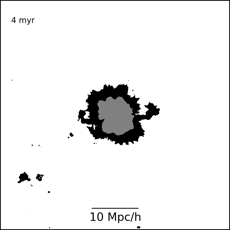
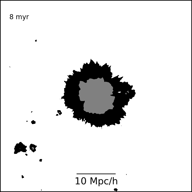
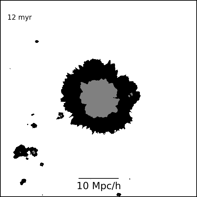
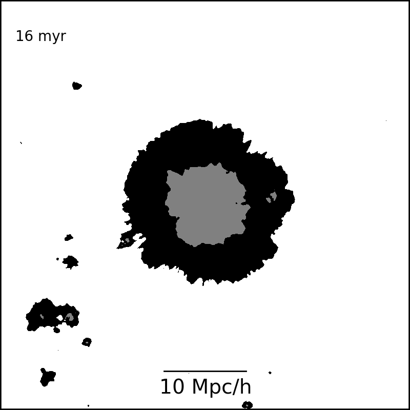
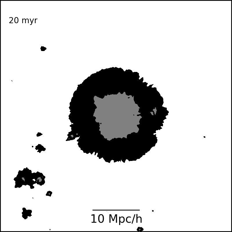
Figure 4: Evolution of the ionization front. The evolution of the ionization front in sub-volume #0 is shown. The ionization front ($x_{\rm HI}\in[0.1,\>0.9]$) is marked in black, and the fully ionized near zone ($x_{\rm HI}<0.1$) is marked with gray.

6.3 MassiveBlack: Spherically Averaged Radius of Ionized Regions

We now examine the results of the radiative transfer post-processing of the eight sub-volumes from MassiveBlack. The averaged CIR radius $\bar{R_{s}}$ for HII and HeIII, as defined in Section 5.2, are shown in Figure 5 as functions of the central source flux. We fit the growth against the scaling relation described by Equation 6, and find that at the low luminosity end (mainly S type and QS type sub-volumes) there is a significant deviation from the fit for the inner and middle fronts.

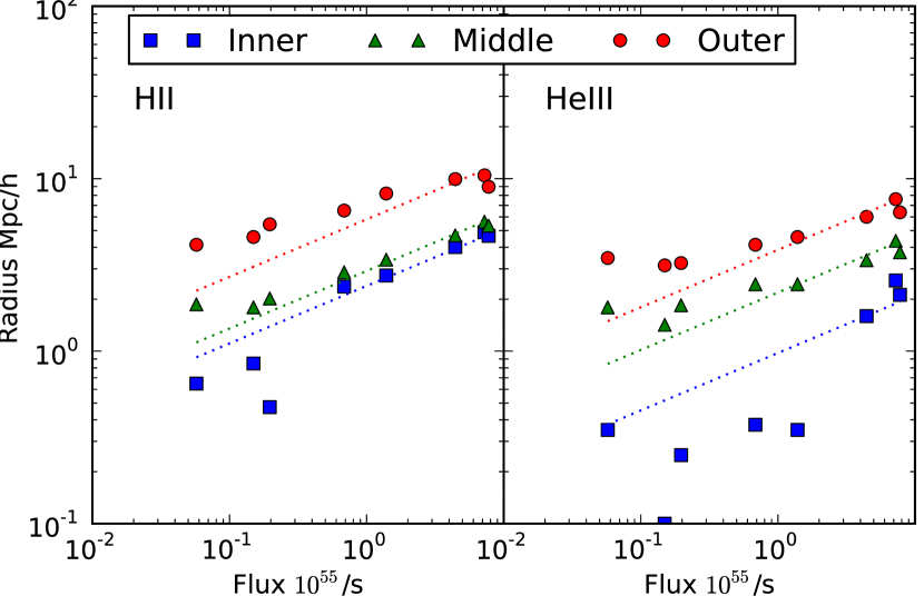
Figure 5: HII and HeIII CIR Front Radius. The left panel is for the HII CIRs, the right panel for the HeIII CIRs. The horizontal axis is the central source flux. The dotted line in the first two panels shows the scaling assuming the analytic model in Equation 6.

The outer front is more extended than the simple uniform density field simulation, albeit given the similar source spectra, hinting that the structure in the IGM is also contributing to the smoothing of the front. This smoothing is a phenomenon similar to that described by Wyithe & Loeb (2007). We also attribute the effect to the clustering of sources; however unlike the smoothing due to secondary ionization, the clustering contribution is anisotropic, and we discuss it in Section 6.4.

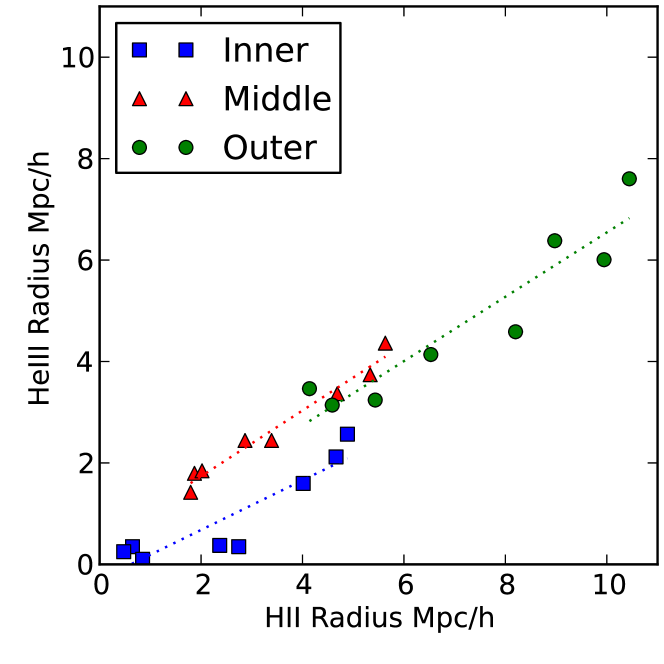
Figure 6: Correlation between HeIII CIR and HII CIR. HeIII CIRs is plotted against HII CIRs, and the linear regression for three fronts are shown with the dotted line.

In Figure 5, we can see that the HII and HeIII CIR radii appear to grow together. The correlation between the two can be seen directly by plotting one against the other, which we do in Figure 6, where we find there is a strong correlation between the HII radius and HeIII radius. The HeIII radius is smaller than the HII radius, agreeing with the finding of Friedrich et al. (2012) who used the ray tracing code C2RAY. We note however that the treatment of secondary ionization and Helium ionization in P-SPHRAY is similar to that of C2RAY, and an agreement is not surprising.

The time evolution history of the HII CIR radius for all sub-volumes is shown in Figure 7. We compare the evolution of the three parts of the fronts with the prediction of the analytic model (in equation 6), in which we have used the clumping factor and mean H density measured within the final CIR in the simulation to estimate a fiducial recombination time $t_{S}$.

The growth of the CIR in the Q type sub-volumes flattens off much earlier than one might expect from a free streaming law. In order to ascertain the relevant physical timescales, we fit the time evolution of the fronts to the full analytic model in 6, and extract the effective recombination time $\hat{t}_{S}$ as a fit parameter, then mark the time in the plot. We can see that for the quasar driven (type Q) sub-volumes, all three fronts (inner, middle and outer) growth stop at about $10\,\mathrm{Myear}$, on the same order of the life time of the quasar $t_{Q}\sim 20\,\mathrm{Myear}$ and the fiducial recombination time $t_{S}\sim 20\,\mathrm{Myear}$. The deviation from free streaming indicates that by merely increasing the life span $t_{Q}$ of the central quasar, we can not substantially increase the size of their CIR.

In S type type sub-volumes, there is a similar tailing off for the inner fronts. However, the outer fronts continue their free streaming growth, behaving differently from the analytic model, which has stopped due to reaching the recombination time. We attribute this apparent excessive growth of the averaged S type outer front to the anisotropic growth via merging with other small ionized bubbles that are close to the CIR, as described later in the paper.

Figure 7: Evolution of three quasar driven sub-volumes. The top panels show the CIR radius as function of time; the thick black line is the fiducial analytic model as described in the text (Equation 6). The vertical short lines show the recombination time in an analytic model as if it is fitted as a parameter to the simulation data points, which are marked with squares (Inner), triangles (Middle), and circles (Outer). The bottom panels show the ratio between the radius and the fiducial model.

We note that our Monte-Carlo RT approach allows for superluminal growth of the CIR. This nonphysical situation happens well before the first snapshot time which is 2 million years after the sources are turned on. The first snapshot, in which the Stromgren sphere typically has grown to about 10% of the full size, gives an upper bound to the contribution from superluminal growth. We conclude that the superluminal growth occurring at early time ($<2\,\mathrm{Myear}$) and small radii ($<10\%$) does not play an important role in the final shape of the ionized bubble. We refer the readers to Shapiro et al. (2006) for a more detailed discussion of the role of the nonphysical superluminal phase of the growth of an ionization front.

6.4 MassiveBlack: Anisotropy of Ionized Regions

In Figure 8 we show the anisotropy measured using Equation 12 of all 8 sub-volumes. The anisotropy of different ionization fronts as a function of radius are marked with different symbols. As a reminder, in Equation 12, the anisotropy $A_{s}$ is the standard deviation of the ionization front radius, so that by comparing to the radius plotted on the x-axis it can be seen that the fronts are not very far from spherical symmetry ($\sim$ 10% variations). We find that larger ionized regions (corresponding to brighter quasar sources) are in general associated with more anisotropy.

In the simulation, the anisotropy of the inner and middle radii of the HII regions do not significantly depend on the radius (the curve is relatively flat), but the outer fronts have more anisotropy. The HeIII regions show a similar feature, except for the inner fronts of three type Q sub-volumes, which have significantly stronger anisotropy.

These phenomena lead us to the following explanation, incorporating two contributing mechanisms:

1. The anisotropic distribution of gas that attenuates the ionizing photons; when the density is high in a particular direction, the extra absorption decreases the radius of the ionized region in that direction.

2. The merging of nearby bubbles from clustered halos; when the density is sufficient to host bright sources lying in a certain direction, their extra photo-ionization increases the bubble radius in that direction. The outer front is more sensitive to merging than the inner and middle front.

For a small CIR (or a CIR in its early growing stage), no merging has occurred and only the density induced anisotropy is present. As the CIR grows, it overlaps with nearby ionized regions, resulting in the second type of anisotropy (due to overlapping). We note that this does not contradict the finding that clustering contributes to the smoothness of the extended ionization front (Wyithe & Loeb, 2007), because by definition, after spherical averaging, the existence of surrounding bubbles will result a smoother averaged front.

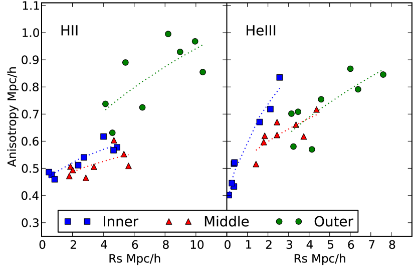
Figure 8: Anisotropy .vs. Radius. The left panel shows the anisotropy of three (inner, middle, outer) HII CIR fronts defined as in Equation 12. The right panel shows the anisotropy of the HeIII fronts. The dotted lines are fits against a square-root + linear offset model and are only meant to guide the eye. All 8 sub-volumes are displayed.

In order to better visualize the structures which cause the anisotropy, we plot the distance to the different parts of the ionization fronts in a Molleweide projection as seen from the point of view of the central source. These maps of the angular-dependent HII bubble radius, $R_{s}$ are shown in Figure 9, where we plot the quasar driven sub-volume 0 and stellar driven sub-volume 4.

Looking from the top panels downwards for sub-volume 0, we can first see clumps of mostly neutral gas close to the quasar which restrict the distance to the $x_{\rm HI}=0.1$ fronts to be very close by ($<1\,\mathrm{Mpc/h}$), compared to the mean distance for this neutral fraction of $\leavevmode\nobreak\ 6\,\mathrm{Mpc/h}$. In the $x_{\rm HI}=0.9$ plot, for sub-volume 0 a prominent red region can be seen at the top. This corresponds to a bubble which has merged with the central bubble. Next to each panel in Figure 9 we show a histogram of the $R_{s}$ values. The secondary bubble is responsible for the small tail of high values region in $x_{\rm HI}=0.9$ histogram, as well as giving an extra contribution to $A_{s}$.

Moving on to the stellar driven sub-volume 4 (right hand panels in Figure 9), we can see that the ionized region radius is smaller by approximately a factor of 3. Because this radius is small compared to the distance to nearby major halos, there is no sign of merging with other large bubbles, and the ionized region remains more isotropic. In the bottom panels of Figure 9 we show the Molleweide-projected mass density within the inscribed sphere of the sub-volume. It is interesting to compare this clumpiness with the structure in the ionized bubble radius. We can see some correlation with some structures, but not as much as might be expected, indicating that the interaction of radiation with the clumpy medium surrounding the sources is a complex process.

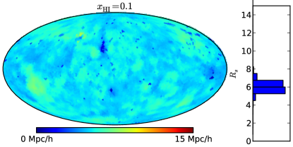
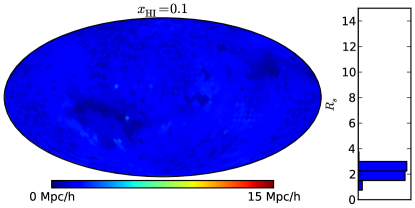
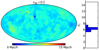
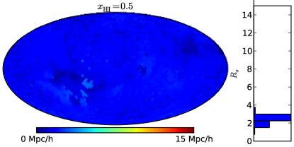
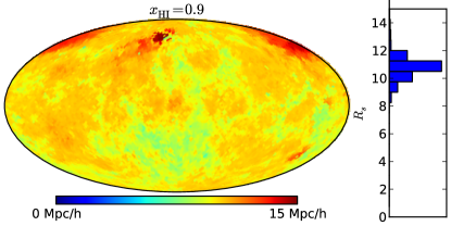
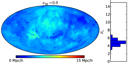
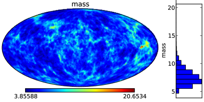
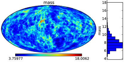
Figure 9: Angular Distribution of the HII Radius. The left column is sub-volume 0 (Q type) and the right column is sub-volume 4 (S type). From top to the bottom the inner ($x_{\rm HI=0.1}$), middle ($x_{\rm HI=0.5}$), and outer ($x_{\rm HI=0.9}$) fronts are shown. The histograms measure the variance of $R_{s}$ in different angles, characterizing the anisotropy. The red region in the $x_{\rm HI}=0.9$ plot of sub-volume 0 is due to merging with a further away HII bubble. The less significant red in the center corresponds to the merging shown in Figure 4.

In Figure 10, we show an orthogonal view to Figure 9, showing structure along rays moving out from the central source in some different directions. The outer HII front radii in three chosen directions are shown as a function of time. This allows us to see in detail how the clustering of halos affects the center bubble radius through merging as the simulation develops. The three directions are (i) one directed towards the second brightest source in the sub-volume, (ii) one directed towards the merging bubble seen on the right hand side of Figure 4, and finally (iii) one oriented in an arbitrarily choosed direction not crossing any nearby secondary bubbles. In order to show the stronger bubble merging effect which would happen with more luminous sources, on the right hand side of Figure 10, we plot the same 3 sight-lines, but after increasing the stellar luminosity by a factor of 10.

Merging happens as the central bubble touches the surrounding ones and meanwhile the radius along that direction significantly increases, compared to the radius without a nearby halo. This can be seen most clearly for sight-line (iii) on the right in Figure 10. The development of the anisotropy due to merging of nearby ionized bubbles is responsible for the apparent rapid growth of the averaged outer Stromgren radius after the growth of the inner radius is stabilized for S type and QS type sub-volumes. As the neutral fraction at the overlapping edge slowly drops below the threshold, two bubbles merge and the averaged radius increases. However, at the luminosity seen in the simulation (left hand panels of Figure 10), such a merging mechanism is mostly limited to the growth of the outer front. It is also worth noting that in the absence of the effect of smoothing due to secondary ionization the steep bubble edges will make the merging even more unlikely.

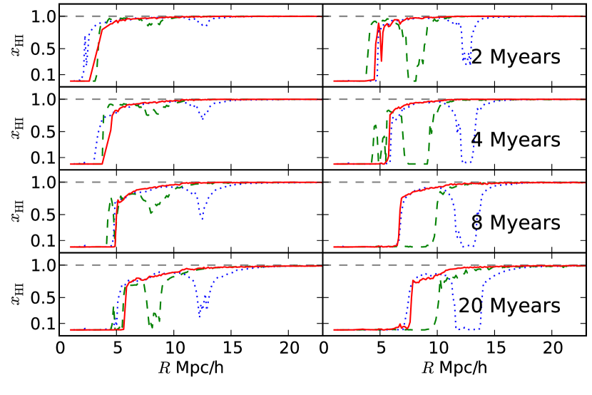
Figure 10: Time evolution of $x_{\rm HI}$. Time evolution of $x_{\rm HI}$ in sub-volume 0, along three selected sight-lines: (i) the blue line is directed towards the second brightest halo in the sub-volume; (ii) the green line is directed towards the merging bubble on the right shown in the slice plots; (iii) the red line is directed towards an arbitrary direction with no nearby bubbles. The left panel is the luminosity model used throughout the paper, while on the right the stellar luminosity is boosted by a factor of 10 to demonstrate a stronger merging effect.

7 Conclusions

We have presented results from radiative transfer simulations in the vicinity of high redshift quasars in the MassiveBlack simulation. We find that the rare brightest quasars drive a much more significant growth of ionized regions than in the purely stellar driven case. The ionized regions associated with active quasars are characterized by (i) a smooth ionized fraction transition from the middle to the outer front, and (ii) an increased anisotropy in the front when it starts to overlap the nearby ionized regions. The nature of such growth is significantly more complex than a simple analytic growth of a single center bubble with clumping correction.

The largest HII bubble obtained in this simulation has a comoving radius of $10\,\mathrm{Mpc/h}$, which is smaller than the general expectation that can fulfill the reionization of the universe (Trac & Gnedin, 2011; Wyithe & Loeb, 2004; Majumdar et al., 2011). The quasar near zones we have presented in this paper are the primordial ancestors of the later much larger Stromgren spheres which will form near the end of the EoR. They are however relatively isolated regions that could be interesting objects for study in future 21cm surveys. After the $z=8$ epoch we have modeled in this paper, we expect that the global star formation in the MassiveBlack simulation increases significantly. This will eventually lead to the global reionization of the universe. We plan to study this process and role of quasars in future work.

Acknowledgments: We acknowledge support from Moore foundation which enabled the radiative transfer simulations to be run at the McWilliams Center of Cosmology at Carnegie Mellon University. The MassiveBlack simulation was run on the Cray XT5 supercomputer Kraken at the National Institute for Computational Sciences. This research has been funded by the National Science Foundation (NSF) PetaApps program, OCI-0749212 and by NSF AST-1009781. We also acknowledge the support of a Leverhulme Trust visiting professorship. The visualizations were produced using Healpix (Górski et al., 2005), Healpy , and Gaepsi (Feng et al., 2011).

Appendix A Source Luminosity Models

A.1 Band luminosity of Quasars

We calculate the bolometric luminosity $L_{{\rm bol}}$ of each quasar from the accretion rate $\dot{M}$ of the super-massive black hole with Equation 3. We choose to use as $\dot{M}$ a single value throughout the calculation, which is averaged accretion rate measured from the simulation over a timescale $t_{Q}=2\times 10^{7}\,\mathrm{yrs,}$ where $t_{Q}$ is also the length of time over which we follow the evolution of the quasar ionization front. We estimate the flux in different bands from the bolometric luminosity according to the fitting formula of Hopkins et al. (2007). The band definitions are listed in Table 3.

Band	Range
UV	$13.6\,\mathrm{eV}$ to $250\,\mathrm{eV}$
Soft X-Ray	$250\,\mathrm{eV}$ to $2\,\mathrm{KeV}$
Hard X-Ray	$2\,\mathrm{eV}$ to $10\,\mathrm{KeV}$

Table 3: Band definitions.

The soft and hard X-Ray band luminosity are directly calculated with the program distributed by Hopkins et al. (2007). We obtain the UV band luminosity from the reported B band luminosity following the broken power law described in the paper ($\alpha_{\rm UV}=1.76$ and $\alpha_{\rm B}=0.44$).

$$L_{\rm UV}=\frac{L_{B}}{\nu_{B}}\left(\frac{\nu_{X}}{\nu_{B}}\right)^{-\alpha_{B}}\left(\frac{\nu_{I}}{\nu_{X}}\right)^{-\alpha_{\rm UV}}\frac{\left(\frac{250}{13.6}\right)^{1-\alpha_{\rm UV}}-1}{1-\alpha_{\rm UV}},$$ (14)

where $\nu_{X}=c/120\,\mathrm{nm}$ is the pivot from optical to UV, $\nu_{B}=c/445\,\mathrm{nm}$ and $\nu_{I}=c/91.1\,\mathrm{nm}$. We calculate the photon flux of the quasar sources according to these power law spectra applied to the various bands.

A.2 Flux of UV stellar photons

The stellar photon flux of a halo is given by

$$\dot{N}_{\rm SFR}=f_{\rm esc}N_{\gamma/\rm H}X_{\rm H}\Phi/m_{p},$$ (15)

where $\Phi$ is the star formation rate of the halo, $X_{\rm H}=0.76$, and $m_{p}$ is the proton mass. We take the escape fraction to be $f_{\rm esc}=0.1$, and the photon to hydrogen ratio to be $N_{\gamma/\rm H}=4000$, a value found to produce a reionization history consistent with observations (Furlanetto et al., 2004; Sokasian et al., 2003). For simplicity, the stellar sources are assigned to the center of the halo; in future work we plan to investigate the effect of the positioning of the stellar sources by either following the star forming gas particles in the simulation directly or the gravitationally bound sub-halos or galaxies. To ease the modeling, we only include and assume the same UV band spectrum for the stellar radiation to that of the quasar spectrum.

References

- Altay et al. (2008) Altay G., Croft R. A. C., Pelupessy I., 2008, MNRAS, 386, 1931
- Alvarez & Abel (2007) Alvarez M. A., Abel T., 2007, MNRAS, 380, L30
- Alvarez et al. (2010) Alvarez M. A., Pen U.-L., Chang T.-C., 2010, ApJ, 723, L17
- Bolton & Haehnelt (2007) Bolton J. S., Haehnelt M. G., 2007, MNRAS, 382, 325
- Bolton et al. (2011) Bolton J. S., Haehnelt M. G., Warren S. J., Hewett P. C., Mortlock D. J., Venemans B. P., McMahon R. G., Simpson C., 2011, MNRAS, 416, L70
- Cen & Haiman (2000) Cen R., Haiman Z., 2000, ApJ, 542, L75
- Chen & Miralda-Escudé (2008) Chen X., Miralda-Escudé J., 2008, ApJ, 684, 18
- Croft & Altay (2008) Croft R. A. C., Altay G., 2008, MNRAS, 388, 1501
- Croft et al. (2001) Croft R. A. C., Di Matteo T., Davé R., Hernquist L., Katz N., Fardal M. A., Weinberg D. H., 2001, ApJ, 557, 67
- Datta et al. (2012) Datta K. K., Friedrich M. M., Mellema G., Iliev I. T., Shapiro P. R., 2012, MNRAS, 424, 762
- Datta et al. (2008) Datta K. K., Majumdar S., Bharadwaj S., Choudhury T. R., 2008, MNRAS, 391, 1900
- DeGraf et al. (2012) DeGraf C., Di Matteo T., Khandai N., Croft R., Lopez J., Springel V., 2012, MNRAS, 424, 1892
- Di Matteo et al. (2008) Di Matteo T., Colberg J., Springel V., Hernquist L., Sijacki D., 2008, ApJ, 676, 33
- Di Matteo et al. (2012) Di Matteo T., Khandai N., DeGraf C., Feng Y., Croft R. A. C., Lopez J., Springel V., 2012, ApJ, 745, L29
- Fan et al. (2006) Fan X., Strauss M. A., Becker R. H., White R. L., Gunn J. E., Knapp G. R., Richards G. T., Schneider D. P., Brinkmann J., Fukugita M., 2006, AJ, 132, 117
- Feng et al. (2011) Feng Y., Croft R. A. C., Di Matteo T., Khandai N., Sargent R., Nourbakhsh I., Dille P., Bartley C., Springel V., Jana A., Gardner J., 2011, ApJS, 197, 18
- Friedrich et al. (2012) Friedrich M. M., Mellema G., Iliev I. T., Shapiro P. R., 2012, MNRAS, 421, 2232
- Furlanetto & Stoever (2010) Furlanetto S. R., Stoever S. J., 2010, MNRAS, 404, 1869
- Furlanetto et al. (2004) Furlanetto S. R., Zaldarriaga M., Hernquist L., 2004, ApJ, 613, 1
- Geil & Wyithe (2008) Geil P. M., Wyithe J. S. B., 2008, MNRAS, 386, 1683
- Giroux & Shapiro (1996) Giroux M. L., Shapiro P. R., 1996, ApJS, 102, 191
- Górski et al. (2005) Górski K. M., Hivon E., Banday A. J., Wandelt B. D., Hansen F. K., Reinecke M., Bartelmann M., 2005, ApJ, 622, 759
- Hopkins et al. (2007) Hopkins P. F., Richards G. T., Hernquist L., 2007, ApJ, 654, 731
- Hui & Gnedin (1997) Hui L., Gnedin N. Y., 1997, MNRAS, 292, 27
- Iliev et al. (2006) Iliev I. T., Ciardi B., Alvarez M. A., Maselli A., Ferrara A., Gnedin N. Y., Mellema G., Nakamoto T., Norman M. L., Razoumov A. O., Rijkhorst E.-J., Ritzerveld J., Shapiro P. R., Susa H., Umemura M., Whalen D. J., 2006, MNRAS, 371, 1057
- Khandai et al. (2012) Khandai N., Feng Y., DeGraf C., Di Matteo T., Croft R. A. C., 2012, MNRAS, 423, 2397
- Loeb (2009) Loeb A., 2009, J. Cosmology Astropart. Phys, 3, 22
- Majumdar et al. (2011) Majumdar S., Choudhury T. R., Bharadwaj S., 2011, ArXiv e-prints
- Maselli et al. (2003) Maselli A., Ferrara A., Ciardi B., 2003, MNRAS, 345, 379
- Maselli et al. (2007) Maselli A., Gallerani S., Ferrara A., Choudhury T. R., 2007, MNRAS, 376, L34
- Mortlock et al. (2011) Mortlock D. J., Warren S. J., Venemans B. P., Patel M., Hewett P. C., McMahon R. G., Simpson C., Theuns T., Gonzáles-Solares E. A., Adamson A., Dye S., Hambly N. C., Hirst P., Irwin M. J., Kuiper E., Lawrence A., Röttgering H. J. A., 2011, Nature, 474, 616
- Pawlik et al. (2009) Pawlik A. H., Schaye J., van Scherpenzeel E., 2009, MNRAS, 394, 1812
- Shapiro & Giroux (1987) Shapiro P. R., Giroux M. L., 1987, ApJ, 321, L107
- Shapiro et al. (2006) Shapiro P. R., Iliev I. T., Alvarez M. A., Scannapieco E., 2006, ApJ, 648, 922
- Shull & van Steenberg (1985) Shull J. M., van Steenberg M. E., 1985, ApJ, 298, 268
- Sokasian et al. (2003) Sokasian A., Abel T., Hernquist L., Springel V., 2003, MNRAS, 344, 607
- Springel & Hernquist (2003) Springel V., Hernquist L., 2003, MNRAS, 339, 289
- Srbinovsky & Wyithe (2007) Srbinovsky J. A., Wyithe J. S. B., 2007, MNRAS, 374, 627
- Thomas & Zaroubi (2008) Thomas R. M., Zaroubi S., 2008, MNRAS, 384, 1080
- Trac & Gnedin (2011) Trac H. Y., Gnedin N. Y., 2011, Advanced Science Letters, 4, 228
- Venkatesan & Benson (2011) Venkatesan A., Benson A., 2011, MNRAS, 417, 2264
- Wyithe & Loeb (2004) Wyithe J. S. B., Loeb A., 2004, Nature, 432, 194
- Wyithe & Loeb (2007) Wyithe J. S. B., Loeb A., 2007, MNRAS, 374, 960