Acoustic radiation- and streaming-induced microparticle velocities determined by micro-PIV in an ultrasound symmetry plane

Abstract

We present micro-PIV measurements of suspended microparticles of diameters from $0.6~{}\textrm{\textmu{}m}$ to $10~{}\textrm{\textmu{}m}$ undergoing acoustophoresis in an ultrasound symmetry plane in a microchannel. The motion of the smallest particles are dominated by the Stokes drag from the induced acoustic streaming flow, while the motion of the largest particles are dominated by the acoustic radiation force. For all particle sizes we predict theoretically how much of the particle velocity is due to radiation and streaming, respectively. These predictions include corrections for particle-wall interactions and ultrasonic thermoviscous effects, and they match our measurements within the experimental uncertainty. Finally, we predict theoretically and confirm experimentally that the ratio between the acoustic radiation- and streaming-induced particle velocities is proportional to the square of the particle size, the actuation frequency and the acoustic contrast factor, while it is inversely proportional to the kinematic viscosity.

I Introduction

Acoustofluidics and ultrasound handling of particle suspensions, recently reviewed in Review of Modern Physics Friend and Yeo (2011) and Lab on a Chip Bruus et al. (2011), is a field in rapid growth for its use in biological applications, such as separation and manipulation of cells and bioparticles. Microchannel acoustophoresis has largely been limited to manipulation of micrometer-sized particles, such as yeast Hawkes et al. (2004), blood cells Petersson et al. (2004), cancer cells Thevoz et al. (2010); Augustsson et al. (2012); Ding et al. (2012), natural killer cells Vanherberghen et al. (2010), and affinity ligand complexed microbeads Augustsson and Laurell (2012), for which the acoustic radiation force dominates. Precise acoustic control of sub-micrometer particles, e.g. small bacteria, vira, and large biomolecules remains a challenge, due to induction of acoustic streaming of the suspending fluid. Nevertheless, acoustic streaming has been used to enhance the convective transport of substrate in a microenzyme reactor for improved efficiency Bengtsson and Laurell (2004), while acoustic manipulation of sub-micrometer particles has been achieved in a few specific cases including enhanced biosensor readout of bacteria Kuznetsova et al. (2005) and bacterial spores Martin et al. (2005), and trapping of E-coli bacteria Hammarstrom et al. (697G).

When a standing ultrasound wave is imposed in a microchannel containing an aqueous suspension of particles, two forces of acoustic origin act on the particles: the Stokes drag force from the induced acoustic streaming and the acoustic radiation force from sound wave scattering on the particles. To date, the experimental work on acoustophoresis has primarily dealt with cases where the acoustic radiation force dominates the motion, typically for particles of diameters larger than $2~{}\textrm{\textmu{}m}$. Quantitative experiments of 5-µm-diameter polymer particles in water Barnkob et al. (2010); Augustsson et al. (2011); Barnkob et al. (2012) have shown good agreement with the classical theoretical predictions Yosioka and Kawasima (1955); Gorkov (1962) of the acoustic radiation force acting on a microparticle of radius $a$ much smaller than the acoustic wavelength $\lambda$, and where the viscosity of the suspending fluid is neglected. However, as the particle diameter is decreased below $2~{}\textrm{\textmu{}m}$, a few times the acoustic boundary-layer thickness, the particle motion is typically strongly influenced by the Stokes drag force from the induced acoustic streaming flow, which has been reported by several groups Wiklund et al. (2012); Spengler et al. (2003); Hagsäter et al. (2007), and the radiation force is modified due to the acoustic boundary layer Settnes and Bruus (2012).

As pointed out in a recent review Wiklund et al. (2012), the acoustic streaming is difficult to fully characterize due to its many driving mechanisms and forms. In acoustofluidic systems, the streaming is primarily boundary-driven arising at rigid walls from the large viscous stresses inside the sub-micrometer-thin acoustic boundary layer of width $\delta$. The boundary-driven acoustic streaming was theoretically treated by Rayleigh Rayleigh (1884) for an isothermal fluid in an infinite parallel-plate channel with a standing wave parallel to the plates of wavelength $\lambda$ much larger than the plate distance $h$, and where $h$ is large compared to $\delta$, i.e. $\lambda\gg h\gg\delta$. However, in many applications of acoustofluidic systems the channels provide enhanced confinement, the acoustic wavelength is comparable to the channel height, and the liquid cannot be treated as being isothermal. Rayleigh’s prediction is often cited, but to our knowledge the literature contains no quantitative validation of its accuracy when applied to acoustofludic systems. This lack of quantitative tests is most likely due to the fact that boundary-driven acoustic streaming is very sensitive to geometry and boundary conditions, making it difficult to achieve sufficient experimental control. However, quantitative comparisons between theory and experiment of acoustic streaming are crucial for the advancement of the acoustofluidics research field. Understanding and controlling the ratio of radiation- and streaming-induced acoustophoretic velocities may be the key for future realization of ultrasound manipulation of sub-micrometer particles.

In 2011, we presented a temperature-controlled micro-PIV setup for accurate measurements of the acoustophoretic microparticle motion in a plane Augustsson et al. (2011). Here, we use the same system and the ability to establish a well-controlled transverse resonance for quantitative studies of how much the radiation- and streaming-induced velocities, respectively, contribute to the total acoustophoretic velocity. More specifically, as illustrated in Fig. 1, we study the microparticle motion in the ultrasound symmetry plane (magenta) of a straight rectangular microchannel of width $w=377~{}\textrm{\textmu{}m}$ and height $h=157~{}\textrm{\textmu{}m}$. We determine the velocities for particles of diameter $2a$ ranging from 0.6 µm to 10 µm, and based on this we examine the validity of Rayleigh’s theoretical streaming prediction. We also derive theoretically and validate experimentally an expression for the microparticle velocity as function of particle size, ultrasound frequency, and mechanical properties of the suspending medium.

II Theory of single-particle acoustophoresis

In this work we study a silicon-glass chip containing a rectangular microchannel sketched in Fig. 1 and described further in Section III. The microchannel contains a particle suspension, and the chip is ultrasonically actuated by attaching a piezo transducer to the chip and driving it with the voltage $U_{\mathrm{pp}}$ at the angular frequency $\omega=2\pi f$, where $f$ is a frequency in the low MHz range. By proper tuning of the applied frequency, the actuation induces a resonant time-harmonic ultrasonic pressure field $p_{1}(\bm{r})\exp{(-\mathrm{i}\omega t)}$ and velocity field $\bm{v}_{1}(\bm{r})\exp{(-\mathrm{i}\omega t)}$, here expressed in the complex time-harmonic notation. Throughout the paper, we only study the case of a 1D transverse pressure resonance of amplitude $p_{\mathrm{a}}$ and wavenumber $k=2\pi/\lambda$,

$$p_{1}(\bm{r})=p_{\mathrm{a}}\>\cos\Big{[}k\Big{(}y-\frac{w}{2}\Big{)}\Big{]}.$$ (1)

The case of $\lambda/2=w$ or $k=\pi/w$ is shown in Fig. 2(a).

The particle suspensions are dilute enough that the particle-particle interactions are negligible, and thus only single-particle effects are relevant. These comprise the acoustic radiation force due to particle-wave scattering and the viscous Stokes drag force from the acoustic streaming flow. Both effects are time-averaged second-order effects arising from products of the first-order fields. The drag force from the acoustic streaming flow dominates the motion of small particles, while the motion of larger particles are dominated by the acoustic radiation force. This is clearly illustrated in recent numerical simulations by Muller et al. Muller et al. (2012), which are reproduced in Fig. 2: (b) the streaming flow advects small particles in a vortex pattern, and (c) radiation force pushes larger particles to the pressure nodal plane at $y=0$.

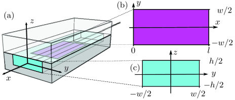
Figure 1: (a) Sketch of the silicon/glass microchip used in our experiments, see also Ref. Augustsson et al. (2011). It contains a straight rectangular water-filled microchannel (light cyan) of length $L=35~{}\textrm{mm}$, width $w=377~{}\textrm{\textmu{}m}$, and height $h=157~{}\textrm{\textmu{}m}$. (b) The horizontal ultrasound symmetry plane (magenta) of length $l=892~{}\textrm{\textmu{}m}$ and width $w$ in the $xy$ plane at the center of the channel. (c) The vertical channel cross section (cyan).

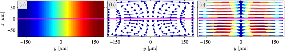
Figure 2: Numerical simulation of microparticle acoustophoresis in the vertical microchannel cross section of Fig. 1(c) adapted from Ref. Muller et al. (2012). The magenta line represents the ultrasound symmetry plane of Fig. 1(b). (a) Color plot of the transverse standing ultrasound pressure wave $p_{1}$ of Eq. (1) ranging from $-p_{a}$ (dark blue) to $p_{a}$ (dark red). (b) Trajectories (blue lines) of small 0.5-µm-diameter particles (dots) dominated by the Stokes drag force from the boundary-induced streaming. (c) Trajectories (colored lines) of large 5.0-µm-diameter particles (dots) dominated by the acoustic radiation force.

II.1 The acoustic radiation force

We consider a spherical particle of radius $a$, density $\rho_{\mathrm{p}}$, and compressibility $\kappa_{\mathrm{p}}$ suspended in a liquid of density $\rho_{0}$, compressibility $\kappa_{0}$, viscosity $\eta$, and momentum diffusivity $\nu=\eta/\rho_{0}$. Recently, Bruus and Settnes Settnes and Bruus (2012) gave an analytical expression for the viscosity-dependent time-averaged radiation force $\bm{F}^{\mathrm{rad}}$ in the experimentally relevant limit of the wavelength $\lambda$ being much larger than both the particle radius $a$ and the thickness $\delta=\sqrt{2\nu/\omega}$ of the acoustic boundary layer, without any restrictions on the ratio $\tilde{\delta}=\delta/a$. For the case of a 1D transverse pressure resonance, Eq. (1), the viscosity-dependent acoustic radiation force on a particle located at $(y,z)$ reduces to the $z$-independent expression

$$F^{\mathrm{rad}}(y,z)=4\pi a^{3}kE_{\mathrm{ac}}\>\Phi(\tilde{\kappa},\tilde{\rho},\tilde{\delta})\>\sin\big{(}2ky\big{)},$$ (2)

where $E_{\mathrm{ac}}=\tfrac{1}{4}\kappa_{0}p^{2}_{\mathrm{a}}$ is the time-averaged acoustic energy density and where the acoustic contrast factor $\Phi$ is given in terms of the material parameters as

$$\Phi(\tilde{\kappa},\tilde{\rho},\tilde{\delta}) =\frac{1}{3}f_{1}(\tilde{\kappa})\!+\!\frac{1}{2}\mathrm{Re}\big{[}f_{2}(\tilde{\rho},\tilde{\delta})\big{]},$$ (3a)

$$f_{1}(\tilde{\kappa}) =1-\tilde{\kappa}, \text{ with }\tilde{\kappa} =\frac{\kappa_{\mathrm{p}}}{\kappa_{0}},$$ (3b)

$$f_{2}(\tilde{\rho},\tilde{\delta}) =\frac{2\big{[}1\!-\!\Gamma(\tilde{\delta})\big{]}(\tilde{\rho}\!-\!1)}{2\tilde{\rho}+1-3\Gamma(\tilde{\delta})}, \text{ with }\tilde{\rho} =\frac{\rho_{\mathrm{p}}}{\rho_{0}},$$ (3c)

$$\Gamma(\tilde{\delta}) =-\frac{3}{2}\Big{[}1+\mathrm{i}(1+\tilde{\delta})\Big{]}\tilde{\delta}, \text{ with }\tilde{\delta} =\frac{\delta}{a}.$$ (3d)

We note that for all the microparticle suspensions studied in this work including the viscous 0.75:0.25 water:glycerol mixture, the viscous corrections to $\Phi$ are negligible as we find $\big{|}\Phi(\tilde{\kappa},\tilde{\rho},\tilde{\delta})/\Phi(\tilde{\kappa},\tilde{\rho},0)-1\big{|}<0.4~{}\%$.

If $\bm{F}^{\mathrm{rad}}$ is the only force acting on a suspended particle, the terminal speed of the particle is ideally given by the Stokes drag as $\bm{u}^{\mathrm{rad}}=\bm{F}^{\mathrm{rad}}/(6\pi\eta a)$. Using Eq. (2) for the transverse resonance, $\bm{u}^{\mathrm{rad}}$ only has a horizontal component $u^{\mathrm{rad}}_{y}$, and this can be written in the form

$$u^{\mathrm{rad}}_{y}=u_{0}\>\frac{a^{2}}{a^{2}_{0}}\>\sin(2ky),$$ (4)

where the characteristic velocity amplitude $u_{0}$ and particle radius $a_{0}$ are given by

$$u_{0} =\frac{4E_{\mathrm{ac}}}{\rho_{0}c_{0}} =\frac{4E_{\mathrm{ac}}}{Z_{0}} =27~{}\textrm{\textmu{}m}\,\textrm{s}^{-1},$$ (5a)

$$a_{0} =\sqrt{\frac{6\nu}{\Phi}\frac{1}{\omega}} =\delta\sqrt{\frac{3}{\Phi}} =1.6~{}\textrm{\textmu{}m}.$$ (5b)

Here, $Z_{0}$ is the characteristic acoustic impedance, and the numerical values are calculated for polystyrene particles suspended in water using parameter values listed in Section III with $f=2~{}\textrm{MHz}$ and $E_{\mathrm{ac}}=10~{}\textrm{J}\>\textrm{m${}^{-3}$}$ as in Barnkob et al. Barnkob et al. (2010, 2012)

II.2 Boundary-driven acoustic streaming

In 1884 Lord Rayleigh Rayleigh (1884) published his now classical analysis of the boundary-driven acoustic streaming velocity field $\bm{U}$ in an infinite parallel-plate channel induced by a first-order bulk velocity field having only a horizontal $y$-component given by $v_{1}=v_{\mathrm{a}}\sin\big{[}k(y-w/2)\big{]}$. This corresponds to the first-order pressure of Eq. (1) illustrated in Fig. 2(a). For an isothermal fluid in the case of $\lambda\gg h\gg\delta$, Rayleigh found the components $U_{y}$ and $U_{z}$ of $\bm{U}$ outside the acoustic boundary to be

$$U_{y}(y,z) =\frac{3}{8}\frac{v^{2}_{\mathrm{a}}}{c_{0}}\sin{(2ky)}\Bigg{[}\frac{3}{2}\frac{z^{2}}{(h/2)^{2}}-\frac{1}{2}\Bigg{]},$$ (6a)

$$U_{z}(y,z) =\frac{3}{16}\frac{v^{2}_{\mathrm{a}}}{c_{0}}kh\cos{(2ky)}\Bigg{[}\frac{z}{(h/2)}-\frac{z^{3}}{(h/2)^{3}}\Bigg{]},$$ (6b)

$$v_{\mathrm{a}} =\frac{p_{\mathrm{a}}}{\rho_{0}c_{0}}=2\sqrt{\frac{E_{\mathrm{ac}}}{\rho_{0}}}.$$ (6c)

A plot of $\bm{U}$ driven by the 1D transverse standing half-wave resonance is shown in Fig. 3. We expect this analytical expression to deviate from our measurements because the actual channel does have side walls, it is not isothermal, and instead of $\lambda\gg h$ we have $\lambda=4.8h$ for $\lambda=2w$ and $\lambda=2.4h$ for $\lambda=w$.

At the ultrasound symmetry plane $z=0$, $\bm{U}$ only has a horizontal component, which we denote $u^{\mathrm{str}}_{y}$. In analogy with Eq. (4) this can be written as

$$u^{\mathrm{str}}_{y}=u_{0}\>s^{0}_{\mathrm{p}}\>\sin(2ky),\quad s^{0}_{\mathrm{p}}=\frac{3}{16}\approx 0.188,$$ (7)

where the sub- and superscript in the streaming coefficient $s^{0}_{\mathrm{p}}$ refer respectively to the parallel-plate geometry and the isothermal liquid in Rayleigh’s analysis.

To estimate the effect on $u^{\mathrm{str}}_{y}$ of the side walls and the large height $h\approx\lambda$ in the rectangular channel of Fig. 1(c), we use the numerical scheme developed by Muller et al. Muller et al. (2012) for calculating the acoustic streaming based directly on the hydrodynamic equations and resolving the acoustic boundary layers, but without taking thermoviscous effects fully into account. The result shown in Fig. 4 reveals that $u^{\mathrm{str}}_{y}$ is suppressed by a factor of 0.82 in the rectangular geometry relative to the parallel-plate geometry and that it approaches zero faster near the side walls at $y=\pm w/2$. The approximate result is

$$u^{\mathrm{str}}_{y}\approx u_{0}\>s^{0}_{\mathrm{r}}\>\sin(2ky),\quad s^{0}_{\mathrm{r}}\approx 0.154,$$ (8)

where the sub- and superscript in the streaming coefficient $s^{0}_{\mathrm{r}}$ refer respectively to the rectangular geometry and the isothermal liquid.

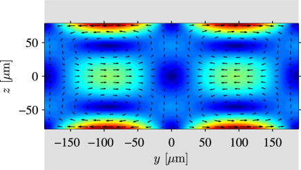
Figure 3: Vector plot (black arrows) of the acoustic streaming $\bm{U}$ and color plot of its magnitude $U$ from zero (dark blue) to maximum (dark red) given by Rayleigh’s analytical expression Eq. (6) and valid for a shallow isothermal liquid slab ($\lambda\gg h$) between two parallel plates (gray) of distance $h$ driven by a standing ultrasound pressure wave $p_{1}=p_{\mathrm{a}}\cos\big{[}k(y-w/2)\big{]}$ for $\lambda/2=w$ or $k=\pi/w$ with $w=377~{}\textrm{\textmu{}m}$.

We estimate the thermoviscous effect on $u^{\mathrm{str}}_{y}$, in particular the temperature dependence of viscosity, using the analytical result by Rednikov and Sadhal for the parallel-plate geometry Rednikov and Sadhal (2011). They found a streaming factor $s^{T}_{\mathrm{p}}$ enhanced relative to $s^{0}_{\mathrm{p}}$,

$$s^{T}_{\mathrm{p}} =\Big{(}1+\frac{2}{3}B_{T}\Big{)}\>s^{0}_{\mathrm{p}}\approx 1.26\>s^{0}_{\mathrm{p}},$$ (9a)

$$B_{T} =(\gamma-1)\Bigg{[}1-\frac{\big{(}\partial_{T}\eta\big{)}_{p}}{\eta\alpha}\Bigg{]}\frac{\sqrt{\nu D_{\mathrm{th}}}}{\nu+D_{\mathrm{th}}},$$ (9b)

where $\alpha$ is the thermal expansion coefficient, $D_{\mathrm{th}}$ the thermal diffusivity, and $\gamma$ the specific heat ratio, and where the value is calculated for water at $T=25~{}^{\circ}\!\textrm{C}$.

Combining the reduction factor 0.82 from the rectangular geometry with the enhancement factor 1.26 from thermoviscous effects leads to $s^{T}_{\mathrm{r}}\approx 1.03\>s^{0}_{\mathrm{p}}$ or

$$u^{\mathrm{str}}_{y}\approx u_{0}\>s^{T}_{\mathrm{r}}\>\sin(2ky),\quad s^{T}_{\mathrm{r}}\approx 0.194,$$ (10)

where the sub- and superscript in the streaming coefficient $s^{T}_{\mathrm{r}}$ refer respectively to the rectangular geometry and a thermoviscous liquid, see Fig. 4.

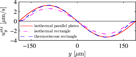
Figure 4: Numerical simulation of the horizontal component $u^{\mathrm{str}}_{y}$ of the streaming velocity in the ultrasound symmetry plane at $z=0$. In this plane the vertical component is zero, $u^{\mathrm{str}}_{z}=0$. Three cases are shown: the isothermal parallel-plate channel Eq. (7), the isothermal rectangular channel Eq. (8), and the thermoviscous rectangular channel Eq. (10).

II.3 Acoustophoretic particle velocity

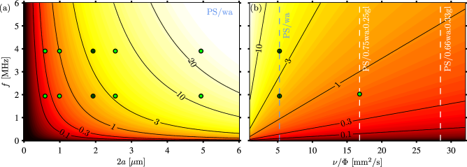
Figure 5: Theoretical prediction of the ratio $u^{\mathrm{rad}}_{y}/u^{\mathrm{str}}_{y}$ Eq. (13) of radiation- and streaming-induced velocities in the ultrasound symmetry plane of the microchannel (magenta in Figs. 1 and 2) at 25 ${}^{\circ}\!\textrm{C}$. (a) Contour plot of $u^{\mathrm{rad}}_{y}/u^{\mathrm{str}}_{y}$ as function of particle diameter $2a$ and ultrasound frequency $f$ for a suspension of polystyrene particles PS in pure water. (b) Contour plot of $u^{\mathrm{rad}}_{y}/u^{\mathrm{str}}_{y}$ as function of $f$ and the rescaled momentum diffusivity $\nu/\Phi$ for fixed particle diameter $2a=2~{}\textrm{\textmu{}m}$. The green dots indicate the cases studied experimentally in Sections III and IV. Suspensions of polystyrene particles in three different liquids are indicated by dashed lines: pure water (light blue) as well as 0.75:0.25 and 0.67:0.33 mixtures of water:glycerol (white).

A single particle undergoing acoustophoresis is directly acted upon by the acoustic radiation force $\bm{F}^{\mathrm{rad}}$, while the acoustic streaming of velocity $\bm{U}$ contributes with a force on the particle through the viscous Stokes drag from the suspending liquid. Inertial effect can be neglected as the characteristic time scale $\rho_{\mathrm{p}}a^{2}/\eta$ of acceleration $(<1~{}\textrm{\textmu{}s}$) is minute in comparison with the time scale of the motion of particles ($>1$ ms). The equation of motion for a spherical particle of velocity $\bm{u}^{\mathrm{p}}$ then becomes

$$\bm{u}^{\mathrm{p}}=\frac{\bm{F}^{\mathrm{rad}}}{6\pi\eta a}+\bm{U}.$$ (11)

As we have seen above, there are no vertical velocity components in the ultrasound symmetry plane at $z=0$, and combining Eqs. (4) and (10) we obtain the horizontal particle velocity component $u^{\mathrm{p}}_{y}$ of amplitude $u_{\mathrm{a}}$,

$$u^{\mathrm{p}}_{y}=u^{\mathrm{rad}}_{y}+u^{\mathrm{str}}_{y}=u_{\mathrm{a}}\>\sin(2ky),\quad u_{\mathrm{a}}=u_{0}\frac{a^{2}}{a^{2}_{0}}+u_{0}\>s,$$ (12)

where we have dropped the sub- and superscripts of the streaming coefficient $s$. The ratio of the radiation- and streaming-induced velocity amplitudes becomes

$$\frac{u^{\mathrm{rad}}_{y}}{u^{\mathrm{str}}_{y}}=\frac{1}{s}\>\frac{a^{2}}{a^{2}_{0}}=\frac{1}{6s}\frac{\Phi}{\nu}\>\omega a^{2},$$ (13)

which scales linearly with the angular frequency $\omega$ and the square $a^{2}$ of the particle radius, but inversely with the streaming coefficient $s$ and the momentum diffusivity $\nu/\Phi$ rescaled by the acoustic contrast factor.

In Fig. 5 we show colored contour plots of the ratio $u^{\mathrm{rad}}_{y}/u^{\mathrm{str}}_{y}$: in (a) for polystyrene particles in water at $25~{}^{\circ}\!\textrm{C}$ as function of the particle diameter $2a$ and the ultrasound frequency $f$, and in (b) as function of $f$ and the rescaled momentum diffusivity $\nu/\Phi$ for fixed particle diameter $2a=2~{}\textrm{\textmu{}m}$. The green dots indicate the experiments described in Sections III and IV.

We define the critical particle diameter $2a_{\mathrm{c}}$ for cross-over from radiation-dominated to streaming-dominated acoustophoresis as the particle diameter for which $u^{\mathrm{rad}}_{y}(a_{\mathrm{c}})=u^{\mathrm{str}}_{y}(a_{\mathrm{c}})$. This results in

$$2a_{\mathrm{c}}=2a_{0}\,\sqrt{s}=\sqrt{\frac{24\nu}{\omega}\frac{s}{\Phi}}\approx 1.4~{}\textrm{\textmu{}m},$$ (14)

where the numerical value is calculated for polystyrene particles in water ($\Phi=0.17$) at $f=2$ MHz using $s=s^{T}_{\mathrm{r}}$. For $a=a_{\mathrm{c}}$ the ratio of the velocity amplitudes $u^{\mathrm{rad}}_{y}/u^{\mathrm{str}}_{y}$ is unity, and consequently the unity contour line in Fig. 5(a) represents $2a_{\mathrm{c}}$ as function of ultrasound frequency $f$.

Table 1: The wall correction factor $\chi$ to the single-particle drag for the particle sizes used in the experiment.

2a	$\chi^{\mathrm{paral}}_{z=0}$	$\chi^{\mathrm{paral}}_{z=\pm h/4}$	$\chi^{\mathrm{perp}}_{\Delta y=w/4}$
$0.6~{}\textrm{\textmu{}m}$	1.004	1.005	1.004
$1.0~{}\textrm{\textmu{}m}$	1.006	1.008	1.006
$1.9~{}\textrm{\textmu{}m}$	1.012	1.016	1.011
$2.6~{}\textrm{\textmu{}m}$	1.017	1.022	1.016
$4.9~{}\textrm{\textmu{}m}$	1.032	1.042	1.030
$10.2~{}\textrm{\textmu{}m}$	1.070	1.092	1.065

II.4 Wall corrections to single-particle drag

The sub-millimeter width and height of the rectangular microchannel enhance the hydrodynamic drag on the microparticles. This problem was treated by Faxén for of a sphere moving parallel to a planar wall or in between a pair of parallel planar walls Faxén (1922) and later extended by Brenner Brenner (1961) to motion perpendicular to a single planar wall, as summarized by Happel and Brenner Happel and Brenner (1983). The enhancement of the Stokes drag is characterized by a dimensionless correction factor $\chi(a)$ modifying Eq. (12),

$$u^{\mathrm{p}}_{y}=\bigg{[}\frac{1}{\chi(a)}\>\frac{a^{2}}{a^{2}_{0}}+s\bigg{]}u_{0}\sin(2ky).$$ (15)

No general analytical form exists for $\chi$, so we list the result for three specific cases. For a particle moving parallel to the surface in the symmetry plane $z=0$ in the gap of height $h$ between two parallel planar walls, $\chi$ is

$$\chi_{z=0}^{\mathrm{paral}}\approx\big{[}1-1.004(2a/h)+0.418(2a/h)^{3}\big{]}^{-1}\approx 1.070,$$ (16)

while for motion in the planes at $z=\pm h/4$ it is

$$\chi_{z=\pm h/4}^{\mathrm{paral}}\approx\big{[}1-1.305(2a/h)+1.18(2a/h)^{3}\big{]}^{-1}\approx 1.092.$$ (17)

Here the numerical values refer to a particle with diameter $2a=10~{}\textrm{\textmu{}m}$ moving in a gap of height $h=157~{}\textrm{\textmu{}m}$. Similarly, for particle motion perpendicular to a single planar wall, the correction factor is

$$\chi^{\mathrm{perp}} =\frac{4}{3}\sinh{(\alpha)}\sum_{n=1}^{\infty}\frac{n(n+1)}{(2n-1)(2n+3)}$$

$$\quad\times\bigg{[}\frac{2\sinh{[(2n+1)\alpha]}+(2n+1)\sinh{(2\alpha)}}{4\sinh^{2}{[(n+\tfrac{1}{2})\alpha]}-(2n+1)^{2}\sinh^{2}{(\alpha)}}-1\bigg{]}$$

$$\approx 1.065,$$ (18)

where $\alpha=\cosh^{-1}(\Delta y/a)$ and $\Delta y$ is the distance from the center of the particle to the wall. The numerical value refers to a 10-µm particle located at $\Delta y=w/4$.

The values of the wall correction factor $\chi$ for all the particle sizes used in this work are summarized in Table 1.

III Experimental procedure

Experiments were carried out to test the validity of the theoretical predictions for the acoustophoretic particle velocity Eq. (15) in the horizontal ultrasound symmetry plane and for the ratio of the corresponding radiation and streaming-induced velocities, see Eq. (13) and Fig. 5.

Table 2: Material parameters at ${T=25~{}^{\circ}\!\textrm{C}}$.

Polystyrene
Density CRCnetBASE Product (2012)	$\rho_{\mathrm{p}}$	$1050~{}\textrm{kg}\>\textrm{m${}^{-3}$}$
Speed of sound Bergmann (1954) (at 20 ${}^{\circ}\!\textrm{C}$)	$c_{\mathrm{p}}$	$2350~{}\textrm{m}\,\textrm{s}^{-1}$
Poisson’s ratio Mott et al. (2008)	$\sigma_{\mathrm{p}}$	$0.35$
Compressibility	$\kappa_{\mathrm{p}}$	$249~{}\mathrm{TPa}^{-1}$
Water
Density CRCnetBASE Product (2012)	$\rho_{0}$	$997~{}\textrm{kg}\>\textrm{m${}^{-3}$}$
Speed of sound CRCnetBASE Product (2012)	$c_{0}$	$1497~{}\textrm{m}\,\textrm{s}^{-1}$
Viscosity CRCnetBASE Product (2012)	$\eta$	$0.890~{}\textrm{mPa}\>\textrm{s}$
Viscous boundary layer, 1.940 MHz	$\delta$	$0.38~{}\textrm{\textmu{}m}$
Viscous boundary layer, 3.900 MHz	$\delta$	$0.27~{}\textrm{\textmu{}m}$
Compressibility	$\kappa_{0}$	$448~{}\mathrm{TPa}^{-1}$
Compressibility factor (polystyrene)	$f_{1}$	$0.444$
Density factor (polystyrene)	$f_{2}$	$0.034$
Contrast factor (polystyrene)	$\Phi$	$0.17$
Rescaled momentum diffusivity (polyst.)	$\nu/\Phi$	$5.25$ mm2 s-1
0.75:0.25 mixture of water and glycerol
Density Cheng (2008)	$\rho_{0}$	$1063~{}\textrm{kg}\>\textrm{m${}^{-3}$}$
Speed of sound Fergusson et al. (1954)	$c_{0}$	$1611~{}\textrm{m}\,\textrm{s}^{-1}$
Viscosity Cheng (2008)	$\eta$	$1.787~{}\textrm{mPa}\>\textrm{s}$
Viscous boundary layer, 2.027 MHz	$\delta$	$0.51~{}\textrm{\textmu{}m}$
Compressibility	$\kappa_{0}$	$363~{}\mathrm{TPa}^{-1}$
Compressibility factor (polystyrene)	$f_{1}$	$0.313$
Density factor (polystyrene)	$f_{2}$	$-0.008$
Contrast factor (polystyrene)	$\Phi$	$0.10$
Rescaled momentum diffusivity (polyst.)	$\nu/\Phi$	$16.8$ mm2 s-1

We use the experimental technique and micro-PIV system as presented in Augustsson et al. Augustsson et al. (2011). The setup is automated and temperature controlled. This enables stable and reproducible generation of acoustic resonances as a function of temperature and frequency. It also enables repeated measurements that lead to good statistics in the micro-PIV analyses. The resulting acoustophoretic particle velocities are thus of high precision and accuracy.

Using the chip sketched in Fig. 1, a total of 22 sets of repeated velocity measurement cycles were carried out on polystyrene particles of different diameters undergoing acoustophoresis in different suspending liquids and at different ultrasound frequencies. In the beginning of each measurement cycle, a particle suspension was infused in the channel while flushing out any previous suspensions. Subsequently, the flow was stopped, and a time lapse microscope image sequence was recorded at the onset of the ultrasound. The cycle was then repeated.

III.1 Microparticle suspensions

Table 3: The nominal and the measured diameter of the polystyrene particles used in the experiment.

Nominal diameter	Measured diameter ($2a$)
591 nm	$(0.59\pm 0.03)~{}\textrm{\textmu{}m}$
992 nm	$(0.99\pm 0.05)~{}\textrm{\textmu{}m}$
2.0 µm	$(1.91\pm 0.07)~{}\textrm{\textmu{}m}$
3.0 µm	$(2.57\pm 0.07)~{}\textrm{\textmu{}m}$
5 µm	$(5.11\pm 0.16)~{}\textrm{\textmu{}m}$
10 µm	$(10.16\pm 0.20)~{}\textrm{\textmu{}m}$

Two types of microparticle suspensions were examined; polystyrene particles suspended in Milli-Q water and polystyrene particles suspended in a 0.75:0.25 mixture of Milli-Q water and glycerol. To each of the two suspending liquids was added 0.01 % w/V Triton-X surfactant. The material parameters of the suspensions are listed in Table 2. Note that the rescaled momentum diffusivity $\nu/\Phi$ of the glycerol suspension is 3 times larger than that for the Milli-Q water suspension.

We analyzed 12 particle suspensions by adding particles of 6 different diameters $2a$ from $0.6~{}\textrm{\textmu{}m}$ to $10~{}\textrm{\textmu{}m}$ to the two liquids. The particle diameters were measured using a Coulter Counter (Multisizer 3, Beckman Coulter Inc., Fullerton, CA, USA) and fitting their distributions to Gaussian distributions, see Supplemental Material. The resulting diameters are listed in Table 3.

The concentration $C$ of the particles were calculated based on the concentrations provided by the manufacturer and varies in this work from $10^{10}~{}\textrm{m}^{-3}$ for the largest particles in the 0.75:0.25 mixture of water and glycerol to $10^{15}~{}\textrm{m}^{-3}$ for the smallest particles in the pure water solution. The concentrations correspond to mean inter particle distances $C^{-1/3}$ ranging from 4 particle diameters for the largest 10-µm particle in water to 173 particle diameters for the smallest 0.6-µm particle in the 0.75:0.25 mixture of water and glycerol. Mikkelsen and Bruus Mikkelsen and Bruus (2005) have reported that hydrodynamic effects become significant for interparticle distances below 2 particle diameters. Thus we can apply the single-particle theory presented in Section II.

III.2 Measurement series

We measured the acoustophoretic velocities of polystyrene microparticles in the following four series of experiments, the second being a repeat of the first:
MQ0: Milli-Q water, $f=1.940~{}\textrm{MHz}$,
$\lambda=2w$, and $2a=1.0$, 1.9, 2.6, and $5.1~{}\textrm{\textmu{}m}$.
MQ1: Milli-Q water, $f=1.940~{}\textrm{MHz}$,
$\lambda=2w$, and $2a=0.6$, 1.0, 1.9, 2.6, 5.1, and $10.2~{}\textrm{\textmu{}m}$.
MQ2: Milli-Q water, $f=3.900~{}\textrm{MHz}$
$\lambda=w$,   and $2a=0.6$, 1.0, 1.9, 2.6, 5.1, and $10.2~{}\textrm{\textmu{}m}$.
GL2: 0.75:0.25 Milli-Q water:glycerol, $f=2.027~{}\textrm{MHz}$
$\lambda=2w$, and $2a=0.6$, 1.0, 1.9, 2.6, 5.1, and $10.2~{}\textrm{\textmu{}m}$.
Given the different particle diameters, we thus have the above-mentioned 22 sets of acoustophoretic particle-velocity measurements, each consisting of 50 to 250 measurement cycles. All experiments were carried out at a fixed temperature of $25~{}^{\circ}\!\textrm{C}$ and the applied piezo voltage $U_{\mathrm{pp}}^{*}$. The camera frame rate was chosen such that the particles would move at least a particle diameter between two consecutive images. The measurement field of view was $1280\times 640$ pixels corresponding to $892~{}\textrm{\textmu{}m}\times 446~{}\textrm{\textmu{}m}$. The imaging parameters were: optical wavelength 520 nm for which the microscope objective is most sensitive, numerical aperture 0.4, and magnification 20. See acquisition details in the Supplemental Material.

III.3 Micro-PIV analysis

The micro-PIV analyses were carried out using the software EDPIV - Evaluation Software for Digital Particle Image Velocimetry, including the image procedure, the averaging in correlation space, and the window shifting described in detail in Ref. Augustsson et al. (2011). For the MQ1, MQ2, and Gl1 series, the interrogation window size was 32 $\times$ 32 pixels with a 50 % overlap resulting in a $79\times 39$ square grid with $16$ pixels between each grid point. For the MQ0 series, the interrogation window size was 64 $\times$ 64 pixels with a 50 % overlap resulting in a $39\times 19$ square grid with $32$ pixels between each grid point.

In micro-PIV all particles in the volume are illuminated, and the thickness of the measurement plane is therefore related to focal depth of the microscope objective. This thickness, denoted the depth of correlation (DOC), is defined as twice the distance from the measurement plane to the nearest plane for which the particles are sufficiently defocused such that it no longer contributes significantly to the cross-correlation analysis Meinhart et al. (2000). The first analytical expression for the DOC was derived by Olsen and Adrian Olsen and Adrian (2000) and later improved by Rossi et al. Rossi et al. (2012). Using the latter, we found that the DOC ranges from $14~{}\textrm{\textmu{}m}$ to $94~{}\textrm{\textmu{}m}\approx h/2$ for the smallest and the largest particles, respectively. Consequently, in the vertical direction all observed particles reside within the middle half of the channel.

IV Results

The core of our results is the 22 discrete acoustophoretic particle-velocity fields obtained by micro-PIV analysis of the 22 sets of acoustic focusing experiments and shown in the Supplemental Material. As in Ref. Augustsson et al. (2011), the measured microparticle velocities $\bm{u}^{\mathrm{p}}$ are thus represented on a discrete $x_{n}\times y_{m}$ micro-PIV grid

$$\bm{u}^{\mathrm{p}}=\bm{u}^{\mathrm{p}}(x_{n},y_{m})=\Bigg{[}\begin{array}[]{c}u^{\mathrm{p}}_{x}(x_{n},y_{m})\\[5.69054pt] u^{\mathrm{p}}_{y}(x_{n},y_{m})\end{array}\Bigg{]}.$$ (21)

All measured velocities presented in the following are normalized to their values at $U_{\mathrm{pp}}=1~{}\textrm{V}$ using the voltage-squared law Barnkob et al. (2010),

$$\bm{u}^{\mathrm{p}}=\bigg{(}\frac{1~{}\textrm{V}}{U_{\mathrm{pp}}^{*}}\bigg{)}^{2}\bm{u}^{\mathrm{p*}},$$ (22)

where the asterisk denotes the actual measured values. As a result, the extracted velocity amplitudes and acoustic energy densities are normalized as well,

$$u_{\mathrm{a}} =\bigg{(}\frac{1~{}\textrm{V}}{U_{\mathrm{pp}}^{*}}\bigg{)}^{2}u_{\mathrm{a}}^{*},$$ (23a)

$$E_{\mathrm{ac}} =\bigg{(}\frac{1~{}\textrm{V}}{U_{\mathrm{pp}}^{*}}\bigg{)}^{2}E_{\mathrm{ac}}^{*}.$$ (23b)

The actual peak-to-peak values of the applied voltage $U_{\mathrm{pp}}^{*}$ for all four experimental series are given in the Supplemental Material.

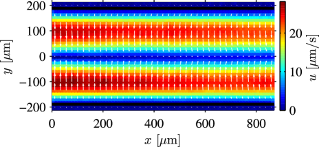
Figure 6: Experimental micro-PIV measurement of acoustophoresis in the horizontal ultrasound symmetry plane of 1-µm-diameter polystyrene particles suspended in water and driven at the piezo frequency $f=1.940~{}\textrm{MHz}$ corresponding to $\lambda/2=w$, temperature $25~{}^{\circ}\!\textrm{C}$, and voltage $U_{\mathrm{pp}}^{*}=7.94~{}\textrm{V}$. The arrows represent the measured velocity vectors $\bm{u}^{\mathrm{p}}$ and the colors their magnitude $u^{\mathrm{p}}$ normalized to $U_{\mathrm{pp}}^{*}$, see Eq. (22).

IV.1 Excitation of a 1D transverse standing wave

In Figs. 6 and 7 we verify experimentally that the acoustophoretic particle velocity is of the predicted sinusoidal form given in Eq. (12) and resulting from a 1D transverse standing wave. For the actual applied voltage of $U_{\mathrm{pp}}^{*}=7.94~{}\textrm{V}$ the maximum velocity was measured to be $1.77~{}\textrm{mm}\,\textrm{s}^{-1}$, which by Eq. (22) is normalized to the maximum velocity $u^{\mathrm{p*}}_{\mathrm{max}}=28~{}\textrm{\textmu{}m}\,\textrm{s}^{-1}$ seen in Fig. 6.

A detailed analysis of the measured velocity field reveals three main points: (i) The average of the ratio of the axial to the transverse velocity component is practically zero, $\langle|u^{\mathrm{p}}_{x}/u^{\mathrm{p}}_{y}|\rangle<5~{}\%$, (ii) the maximum particle velocity along any line with a given axial grid point coordinate $x_{m}$ varies less than $6~{}\%$ as a function of $x_{m}$, and (iii) the axial average $\langle u^{\mathrm{p}}_{y}\rangle_{x}$ of the transverse velocity component $u^{\mathrm{p}}_{y}$ is well fitted within small errorbars ($<1$ %) by Eq. (12).

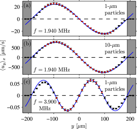
Figure 7: Measured average $\langle u^{\mathrm{p}}_{y}\rangle_{x}$ (black and red points) and its standard deviation $\sigma(\langle u^{\mathrm{p}}_{y}\rangle_{x})$ (error bars) of the transverse velocity $u^{\mathrm{p}}_{y}$ of polystyrene particles in water. The sinusoidal prediction Eq. (12) for $u^{\mathrm{p}}$ (blue line) is fitted to data points $\langle u^{\mathrm{p}}_{y}\rangle_{x}$ away from the side walls (red points). (a) Streaming-dominated acoustophoresis for $2a=1~{}\textrm{\textmu{}m}$ driven at $f=1.940~{}\textrm{MHz}$ ($\lambda/2=w$, same data as in Fig. 6). (b) Radiation-dominated acoustophoresis for $2a=10~{}\textrm{\textmu{}m}$ at $f=1.940~{}\textrm{MHz}$ ($\lambda/2=w$). (c) Streaming-dominated acoustophoresis for $2a=1~{}\textrm{\textmu{}m}$ at $f=3.900~{}\textrm{MHz}$ ($\lambda=w$).

IV.2 Measuring the velocity amplitude

In Fig. 7(a) we plot the axial average $\langle u^{\mathrm{p}}_{y}\rangle_{x}$ of the transverse velocity component $u^{\mathrm{p}}_{y}$ (black and red points) and its standard deviation $\sigma(\langle u^{\mathrm{p}}_{y}\rangle_{x})$ (error bars) for the velocity field shown in Fig. 6 at the standing half-wave resonance frequency $f=1.940~{}\textrm{MHz}$ for the 1-µm-diameter streaming-dominated particles (series MQ1). The measured velocities away from the side walls (red points) are fitted well by the predicted sinusoidal velocity profile $u_{\mathrm{a}}\sin(2ky)$ (blue curve) Eq. (12) for fixed wavelength $\lambda=2\pi/k=2w$ and using $u_{\mathrm{a}}$ as the only fitting parameter. Velocities close to the side walls (black points) are discarded due to their interaction with the side walls. As seen numerically in Fig. 4, the no-slip boundary condition on the side walls of the rectangular geometry suppresses the streaming velocity near the side walls relative to sinusoidal velocity profile of the parallel-plate geometry.

As shown in Fig. 7(b), the theoretical prediction also fits well the measured velocities away from the side walls for the large radiation-dominated 10-µm-diameter particles (series MQ1, $\lambda/2=w$). Likewise, as seen in Fig. 7(c), a good fit is also obtained for the 1-µm-diameter particles away from the side walls at the standing full-wave frequency $f=3.900~{}\textrm{MHz}$ (series MQ2, $\lambda=w$).

Given this strong support for the presence of standing transverse waves, we use this standing-wave fitting procedure to determine the velocity amplitude $u_{\mathrm{a}}$ in the following analysis of the acoustophoretic particle velocity.

In spite of the normalization to the same driving voltage of 1 V, the velocity amplitude of the half-wave resonance in Fig. 7(a) is 400 times larger than that of the full-wave resonance in Fig. 7(c). This is due to a difference in coupling to the piezo and in dissipation.

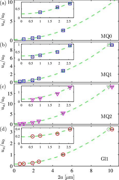
Figure 8: Measured and normalized acoustophoretic velocity amplitudes $u_{\mathrm{a}}/u_{0}$ as function of particle diameter $2a$ (colored symbols) and wall-drag-corrected particle diameter $2a_{\mathrm{wd}}$ (gray symbols) for the four experiment series (a) MQ0, (b) MQ1, (c) MQ2 and (d) Gl1 described in Section III.2. The characteristic velocity amplitude $u_{0}$ is determined from fitting Eq. (12) to the gray points in each series using $E_{\mathrm{ac}}$ and $s$ as fitting parameters resulting in the values listed in Table 4(a) (green dashed lines). The standard deviation of $u_{\mathrm{a}}/u_{0}$ is less than the symbol size and the standard deviations on the particle diameters are indicated as black lines.

Table 4: Measured acoustic energy densities $E_{\mathrm{ac}}$ normalized to $U_{\mathrm{pp}}=1~{}\textrm{V}$ and streaming coefficient $s$.

(a) Un-weighted fit to all points, see Fig. 8.
Susp., freq.	$E_{\mathrm{ac}}$ [J m-3]	$s$
MQ0, 1.940 MHz	52.306 $\pm$ 0.918	0.222 $\pm$ 0.025
MQ1, 1.940 MHz	31.807 $\pm$ 0.569	0.247 $\pm$ 0.071
MQ2, 3.900 MHz	0.070 $\pm$ 0.001	0.262 $\pm$ 0.125
Gl1, 2.027 MHz	2.420 $\pm$ 0.020	0.184 $\pm$ 0.012
(b) Based on particles with $2a=0.6~{}\textrm{\textmu{}m}$ and $2a=10~{}\textrm{\textmu{}m}$
Susp., freq.	$E_{\mathrm{ac}}$ [J m-3]	$s$
MQ1, 1.940 MHz	32.436 $\pm$ 1.282	0.182 $\pm$ 0.008
MQ2, 3.900 MHz	0.071 $\pm$ 0.003	0.205 $\pm$ 0.008
Gl1, 2.027 MHz	2.559 $\pm$ 0.110	0.186 $\pm$ 0.008

IV.3 Velocity as function of particle diameter

To analyze in detail the transverse velocity amplitude $u_{\mathrm{a}}$ in all four series MQ0, MQ1, MQ2, and Gl1, we return to the wall-enhanced drag coefficient $\chi$ of Section II.4. In general, $\chi$ depends in a non-linear way on the motion and position of the particle relative to the rigid walls. However, in Section III.3 we established that the majority of the observed particles reside in the middle half of the channel, and in our standing-wave fitting procedure for $u_{\mathrm{a}}$ in Section IV.2 we discarded particles close to the side walls. Consequently, given this and the values of $\chi$ in Table 1, it is a good approximation to assume that all involved particles have the same wall correction factor, namely the symmetry-plane, parallel-motion factor,

$$\chi\approx\chi^{\mathrm{paral}}_{z=0}.$$ (24)

As the drag-correction only enters on the radiation-induced term in Eq. (15), we introduce a wall-drag-corrected particle size $a_{\mathrm{wd}}=(\chi^{\mathrm{paral}}_{z=0})^{-\frac{1}{2}}\>a$.

To determine the acoustic energy density $E_{\mathrm{ac}}$ and the streaming coefficient $s$ we plot in Fig. 8, for each of the four experiment series, $u_{\mathrm{a}}/u_{0}$ versus the particle diameter $2a$ (colored symbols) and wall-drag-corrected particle diameter $2a_{\mathrm{wd}}$ (gray symbols). The characteristic velocity amplitude $u_{0}$ is determined in each series by fitting the wall-drag-corrected data points to Eq. (12) using $E_{\mathrm{ac}}$ and $s$ as fitting parameters. In all four experiment series, a clear $a^{2}$-dependence is seen. Notice further that the velocities follow almost the same distribution around the fitted line in all series. This we suspect may be due to systematic errors, e.g.  that the 5-µm-diameter particles are slightly underestimated (see the Coulter data in Supplemental Material). The resulting fitting parameters $E_{\mathrm{ac}}$ and $s$ are listed in Table 4(a). The energy densities normalized to $U_{\mathrm{pp}}=1~{}\textrm{V}$, see Eq. (23b) varies with more than a factor 700 due to a large difference in the strength of the excited resonances. According to the predictions in Section II the streaming coefficient $s$ should be constant, but experimentally it varies from $0.18$ to $0.25$. However, taking the fitting uncertainties into account in a weighted average, leads to $\langle s\rangle_{\mathrm{w}}=0.192\pm 0.010$ close to $s^{T}_{\mathrm{r}}\approx 0.194$ of Eq. (10).

Another approach for extracting $E_{\mathrm{ac}}$ and $s$ is to assume that the smallest particles $2a=0.6~{}\textrm{\textmu{}m}$ are influenced only by the streaming-induced drag. If so, the velocity of the largest $2a=10~{}\textrm{\textmu{}m}$ particle has a streaming component of less than $6~{}\%$, see the measured ratios $u_{\mathrm{a}}^{0.6~{}\textrm{\textmu{}m}}/u_{\mathrm{a}}^{10~{}\textrm{\textmu{}m}}$ in Table 5. Therefore, we further assume that the $10~{}\textrm{\textmu{}m}$-diameter particles are influenced solely by the radiation force, and from $u_{\mathrm{a}}^{\mathrm{rad}}=u_{\mathrm{a}}(a/a_{0})^{2}$ we determine the acoustic energy density as

$$E_{\mathrm{ac}}=\frac{3}{2}\frac{\eta c_{0}}{\Phi\omega}\frac{u_{\mathrm{a}}^{10~{}\textrm{\textmu{}m}}}{a_{\mathrm{wd}}^{2}}.$$ (25)

Knowing the acoustic energy density, we use Eq. (7) to calculate the streaming coefficient $s$ from $u_{\mathrm{a}}^{\mathrm{str}}=u_{0}s$ as

$$s =\frac{\rho_{0}c_{0}}{4E_{\mathrm{ac}}}u^{\mathrm{0.6~{}\textrm{\textmu{}m}}}_{a}.$$ (26)

Assuming that the largest error is due to the dispersion in particle size, we obtain the results listed in Table 4(b). The acoustic energy densities are close to the ones extracted from the fits in Fig. 8 and the geometric streaming coefficient varies from 0.180 to 0.203 with an weighted average of $\langle s\rangle_{\mathrm{w}}=0.191\pm 0.005$. Note that using Eqs. (25) and (26), we only need to consider the dispersion of the 10-µm-diameter particles, which results in a more reliable estimate of $s$.

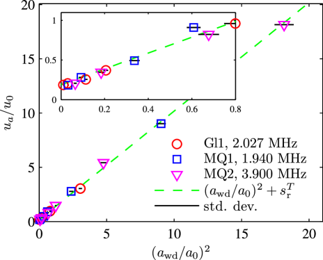
Figure 9: Normalized acoustophoretic particle velocities $u_{\mathrm{a}}/u_{0}$ versus normalized particle size squared $(a_{\mathrm{wd}}/a_{0})^{2}$.

We use the acoustic energy densities in Table 4(b) together with the material parameters in Table 2 to calculate $u_{0}$ and $a_{0}$, Eq. (5), for each of the experiment series MQ1, MQ2, and Gl1. According to the theoretical prediction in Eq. (12), all data points must fall on a straight line of unity slope and intersection $s$ if plotted as the normalized velocity amplitude $u_{\mathrm{a}}/u_{0}$ as function of the normalized particle radius squared $(a/a_{0})^{2}$. The plot is shown in Fig. 9 showing good agreement with the theoretical prediction using $s^{T}_{\mathrm{r}}\approx 0.194$.

Table 5: Relative particle velocities.

Susp., freq.	$\frac{u_{\mathrm{a}}^{0.6~{}\textrm{\textmu{}m}}}{u_{\mathrm{a}}^{10~{}\textrm{\textmu{}m}}}$	$\frac{u_{\mathrm{a}}^{10~{}\textrm{\textmu{}m}}}{u_{\mathrm{a}}^{0.6~{}\textrm{\textmu{}m}}}$	$\frac{u_{\mathrm{a}}^{5~{}\textrm{\textmu{}m}}-u_{\mathrm{a}}^{0.6~{}\textrm{\textmu{}m}}}{u_{\mathrm{a}}^{10~{}\textrm{\textmu{}m}}-u_{\mathrm{a}}^{0.6~{}\textrm{\textmu{}m}}}$
MQ1, 1.940 MHz	0.020	49.6	0.294
MQ2, 3.900 MHz	0.011	88.4	0.291
Gl1, 2.027 MHz	0.061	16.4	0.270

IV.4 Velocity ratios

In Table 5 we list velocity ratios for different particle sizes in the experiment series MQ1, MQ2, and Gl1.

From Eq. (12) we expect $u_{\mathrm{a}}-u_{\mathrm{a}}^{\mathrm{str}}\propto a^{2}$ leading to the prediction $(u_{\mathrm{a}}^{5~{}\textrm{\textmu{}m}}-u_{\mathrm{a}}^{\mathrm{str}})/(u_{\mathrm{a}}^{10~{}\textrm{\textmu{}m}}-u_{\mathrm{a}}^{\mathrm{str}})=(5/10)^{2}=0.25$. If we assume that the smallest 0.6-µm-diameter particles are only influenced by the acoustic streaming, we have $u_{\mathrm{a}}^{\mathrm{str}}=u_{\mathrm{a}}^{0.6~{}\textrm{\textmu{}m}}$. We can therefore test the just mentioned hypothesis by calculating $(u_{\mathrm{a}}^{5~{}\textrm{\textmu{}m}}-u_{\mathrm{a}}^{0.6~{}\textrm{\textmu{}m}})/(u_{\mathrm{a}}^{10~{}\textrm{\textmu{}m}}-u_{\mathrm{a}}^{0.6~{}\textrm{\textmu{}m}})$. The results are listed in the third column in Table 5, where we obtain values ranging from 0.27 to to 0.29, or a deviation of 8 to 18 %.

Assuming that the smallest 0.6-µm-diameter particles and the largest 10-µm-diameter particles are influenced only by the acoustic streaming and the acoustic radiation force, respectively, we can estimate the ratio of radiation- and streaming-induced velocities as $u_{\mathrm{a}}^{\mathrm{rad}}/u_{\mathrm{a}}^{\mathrm{str}}=u_{\mathrm{a}}^{10~{}\textrm{\textmu{}m}}/u_{\mathrm{a}}^{0.6~{}\textrm{\textmu{}m}}$, which are listed in the second column in Table 5. First, we notice that the ratio increases by a factor of $88.4/49.6=1.8$ as we increase the frequency by a factor of $3.900/1.940=2.0$. This agrees well with a linear increase with frequency as predicted by Eq. (13). Secondly, we notice that the ratio increases by a factor of $48.6/16.4=3.0$ as we change the suspending medium from a 0.75:0.25 mixture of water and glycerol to pure water. According to Eq. (13) $u_{\mathrm{a}}^{\mathrm{rad}}/u_{\mathrm{a}}^{\mathrm{str}}$ increases linearly with $\nu/\Phi$ and from Table 2 we obtain a predicted ratio increase of $16.8/5.25=3.2$, which matches well with the experimentally-estimated ratio.

With these results we have gained experimental support for the theoretical prediction of the velocity ratio given in Eq. (13).

V Discussion

Our results verify experimentally the theoretically predicted dependence of the magnitude of the acoustophoretic velocity in a microchannel on the viscosity of the suspending liquid, the acoustic contrast factor $\Phi$, and the ultrasound frequency.

For most situations involving cells, isotonic solutions are used such as PBS, sodium chloride, or blood plasma. Direct manipulation of small particles such as bacteria in plasma or in buffers of high levels of protein is problematic, primarily due to the high viscosity of those media. When possible, these media should be exchanged prior to manipulation to increase the potential for success.

Increasing the frequency in the system would allow for a reduction of the critical diameter of particles. One adverse effect of a higher frequency is that the channel width must be narrowed down which affect the throughput in the system. This problem can, however, be overcome by designing a channel of high aspect ratio, where the resonance occurs over the smallest dimension Adams et al. (2012).

Another benefit of high aspect ratio channels was pointed out by Muller et al. Muller et al. (2012). Since the acoustic streaming emanates from the walls perpendicular to the wave propagation, here the top and bottom, a high channel leads to a weaker average streaming field in the center.

The measurements of particle velocities for polystyrene particles ranging from $0.6~{}\textrm{\textmu{}m}$ to $10~{}\textrm{\textmu{}m}$ give no support to previous measurements presented by Yasuda and Kamakura Yasuda and Kamakura (1997) in 1997. Their rather spectacular result was that particles below a certain size move faster than larger particles do. From the experiments reported herein it is clear, however, that the motion of particles indeed can be well described with the analyses presented by Rayleigh Rayleigh (1884), Yosioka and Kawasima Yosioka and Kawasima (1955), and Gorkov Gorkov (1962).

The uncertainties in the measured particle velocities may in particular be due to the following four causes: (i) Variations in particle density $\rho_{\mathrm{p}}$ and compressibility $\kappa_{\mathrm{p}}$ as function of particle producer (Fluka and G. Kisker) or batch, (ii) deviations from normal distributed particle sizes as shown in Supplemental Material Fig. 1, (ii) local fluctuations in the bead concentrations leading to particle-particle interactions, and (iv) viscosity variations induced by the suspended particles.

To better understand the nature of acoustic streaming in microchannels the streaming field should be mapped for the channel cross section and along the whole length of the channel. As reported by Hagsäter et al.  Hagsäter et al. (2008) and Augustsson et al. Augustsson et al. (2011) the acoustic field can deviate dramatically from the very uniform one dimensional field reported herein. Non symmetrical acoustic fields can be expected to generate far more complex streaming fields.

VI Conclusions

We have investigated the motion of microparticles due to acoustic radiation and acoustic streaming inside a liquid-filled long, straight rectangular channel of width $w$ and height $h$ driven by an ultrasound standing wave of wavelength $\lambda$ .

Fortuitously, the simple analytical expression derived by Lord Rayleigh for the streaming velocity in an isothermal liquid slab between two infinite parallel plates fulfilling $\lambda\gg h$, is a good approximation for the specific rectangular channel of Fig. 1 containing a thermoviscous liquid and fulfilling $\lambda\approx h$. The reduction in velocity obtained when substituting the parallel plates with the rectangular geometry is almost perfectly compensated for by the enhancement in velocity from substituting the isothermal liquid by the thermoviscous one.

A theoretical prediction was made, Eq. (12), for the dependence of the radiation- and streaming-induced velocities on the size of the particles, the ultrasound frequency, the viscosity of the suspending liquid, and the acoustic contrast factor. This prediction was found to be in excellent agreement with experimental findings as shown by the collapse after re-scaling of data from 22 different measurement on the same line in Fig. 9. The results have bearing on acoustophoretic manipulation strategies for sub-micrometer biological particles such as bacteria and vira, which are too small to be handled using the present manifestation of this technique. We can conclude that increasing the ultrasound frequency, increase of the channel aspect ratio, and lowering the viscosity of the suspending fluid is probably the most viable route to conduct such manipulation.

References

- Friend and Yeo (2011) J. Friend and L. Y. Yeo, Rev Mod Phys 83, 647 (2011).
- Bruus et al. (2011) H. Bruus, J. Dual, J. Hawkes, M. Hill, T. Laurell, J. Nilsson, S. Radel, S. Sadhal, and M. Wiklund, Lab Chip 11, 3579 (2011).
- Hawkes et al. (2004) J. J. Hawkes, R. W. Barber, D. R. Emerson, and W. T. Coakley, Lab Chip 4, 446 (2004).
- Petersson et al. (2004) F. Petersson, A. Nilsson, C. Holm, H. Jönsson, and T. Laurell, Analyst 129, 938 (2004).
- Thevoz et al. (2010) P. Thevoz, J. D. Adams, H. Shea, H. Bruus, and H. T. Soh, Anal Chem 82, 3094 (2010).
- Augustsson et al. (2012) P. Augustsson, C. Magnusson, M. Nordin, H. Lilja, and T. Laurell, Anal. Chem. in press (2012).
- Ding et al. (2012) X. Ding, S.-C. S. Lin, B. Kiraly, H. Yue, S. Li, I.-K. Chiang, J. Shi, S. J. Benkovic, and T. J. Huang, PNAS 109, 11105 (2012).
- Vanherberghen et al. (2010) B. Vanherberghen, O. Manneberg, A. Christakou, T. Frisk, M. Ohlin, H. M. Hertz, B. Onfelt, and M. Wiklund, Lab Chip 10, 2727 (2010).
- Augustsson and Laurell (2012) P. Augustsson and T. Laurell, Lab Chip 12, 1742 (2012).
- Bengtsson and Laurell (2004) M. Bengtsson and T. Laurell, Anal Bioanal Chem 378, 1716 (2004).
- Kuznetsova et al. (2005) L. a. Kuznetsova, S. P. Martin, and W. T. Coakley, Biosensors & bioelectronics 21, 940 (2005).
- Martin et al. (2005) S. P. Martin, R. J. Towsend, L. A. Kuznetsova, K. A. J. Borthwick, M. Hill, M. B. McDonnell, and W. T. Coakley, Biosens Bioelectron 21, 758 (2005).
- Hammarstrom et al. (697G) B. Hammarstrom, T. Laurell, and J. Nilsson, Lab Chip 12, in press (2012, doi: 10.1039/C2LC40697G).
- Barnkob et al. (2010) R. Barnkob, P. Augustsson, T. Laurell, and H. Bruus, Lab Chip 10, 563 (2010).
- Augustsson et al. (2011) P. Augustsson, R. Barnkob, S. T. Wereley, H. Bruus, and T. Laurell, Lab Chip 11, 4152 (2011).
- Barnkob et al. (2012) R. Barnkob, I. Iranmanesh, M. Wiklund, and H. Bruus, Lab Chip 12, 2337 (2012).
- Yosioka and Kawasima (1955) K. Yosioka and Y. Kawasima, Acustica 5, 167 (1955).
- Gorkov (1962) L. P. Gorkov, Soviet Physics - Doklady 6, 773 (1962).
- Wiklund et al. (2012) M. Wiklund, R. Green, and M. Ohlin, Lab Chip 12, 2438 (2012).
- Spengler et al. (2003) J. F. Spengler, W. T. Coakley, and K. T. Christensen, AIChE J 49, 2773 (2003).
- Hagsäter et al. (2007) S. M. Hagsäter, T. G. Jensen, H. Bruus, and J. P. Kutter, Lab Chip 7, 1336 (2007).
- Settnes and Bruus (2012) M. Settnes and H. Bruus, Phys Rev E 85, 016327 (2012).
- Rayleigh (1884) L. Rayleigh, Philosophical Transactions of the Royal Society of London 175, 1 (1884).
- Muller et al. (2012) P. B. Muller, R. Barnkob, M. J. H. Jensen, and H. Bruus, Lab Chip 12, in press (2012).
- Rednikov and Sadhal (2011) A. Y. Rednikov and S. S. Sadhal, Journal of Fluid Mechanics 667, 426 (2011).
- Faxén (1922) H. Faxén, Ann Phys 68, 89 (1922).
- Brenner (1961) H. Brenner, Chem Eng Sci 16, 242 (1961).
- Happel and Brenner (1983) J. Happel and H. Brenner, Low Reynolds number hydrodynamics with special applications to particulate media (Martinus Nijhoff Publishers, The Hague, 1983).
- CRCnetBASE Product (2012) CRCnetBASE Product, CRC Handbook of Chemistry and Physics, 92nd ed. (Taylor and Francis Group, www.hbcpnetbase.com/, 2012).
- Bergmann (1954) L. Bergmann, Der Ultraschall und seine Anwendung in Wissenschaft und Technik, 6th ed. (S. Hirzel Verlag, Stuttgart, 1954).
- Mott et al. (2008) P. H. Mott, J. R. Dorgan, and C. M. Roland, J Sound Vibr 312, 572 (2008).
- Landau and Lifshitz (1986) L. D. Landau and E. M. Lifshitz, Theory of Elasticity. Course of Theoretical Physics, 3rd ed., Vol. 7 (Pergamon Press, Oxford, 1986).
- Cheng (2008) N.-S. Cheng, Ind Eng Chem Res 47, 3285 (2008).
- Fergusson et al. (1954) F. Fergusson, E. Guptill, and A. MacDonald, J Acoust Soc Am 26, 67 (1954).
- Mikkelsen and Bruus (2005) C. Mikkelsen and H. Bruus, Lab Chip 5, 1293 (2005).
- Meinhart et al. (2000) C. Meinhart, S. Wereley, and M. Gray, Measurement Science and Technology 11, 809 (2000).
- Olsen and Adrian (2000) M. G. Olsen and R. J. Adrian, Exp Fluids Suppl., S166 (2000).
- Rossi et al. (2012) M. Rossi, R. Segura, C. Cierpka, and C. J. Kaehler, Experiments in Fluids 52, 1063 (2012).
- Adams et al. (2012) J. D. Adams, C. L. Ebbesen, R. Barnkob, A. H. J. Yang, H. T. Soh, and H. Bruus, J Micromech Microeng 22, 075017 (2012).
- Yasuda and Kamakura (1997) K. Yasuda and T. Kamakura, Applied physics letters 71, 1771 (1997).
- Hagsäter et al. (2008) S. M. Hagsäter, A. Lenshof, P. Skafte-Pedersen, J. P. Kutter, T. Laurell, and H. Bruus, Lab Chip 8, 1178 (2008).