Critical phenomena of the Majority voter model in a three dimensional cubic lattice

Abstract

In this work we investigate the critical behavior of the three dimensional simple-cubic Majority voter model. Using numerical simulations and a combination of two different cumulants we evaluated the critical point with a higher accuracy than the previous numerical result found by Yang et al.  [J.-S. Yang, I.-M. Kim and W. Kwak, Phys. Rev. E 77, 051122 (2008)]. Using standard Finite Size Scaling theory and scaling corrections we find that the critical exponents $\nu,\gamma$ and $\beta$ are the same as those of the three dimensional Ising model.

I INTRODUCTION

The Majority Voter (MV) model is one of the simplest non-equilibrium models that present a second order phase transition, and its critical exponents for a two-dimensional square lattices are the same as those of the Ising model Oliveira92 ; Kwak2007 . Those results confirm the conjecture that non equilibrium models with up-down symmetry and spin flip dynamics fall within the universality class of the equilibrium Ising model Grinstein . However, other numerical results suggest that the MV on non-regular lattices does not belong to the Ising universality class Campos2003 ; Lima2005 ; Lima2006 ; Wu2010 .

In a recent work Yang et al. Yang2008 carried out Monte Carlo simulations for the MV model on regular lattices from three to seven dimensions, and they found that the critical exponents differ from the Ising ones below $d=6$. Based on this results they suggest that the upper critical dimension for the MV model is 6 instead of 4. This is a really important result that requires verification, since it implies the existence of a new universality class for Ising-like spin systems in regular lattices. Another result that raises some concerns relates to the Rushbrooke and Josephson hyperscaling relation, which is not satisfied with the reported exponents for the three-dimensional case. In fact, Yang2008 obtains $(2\beta+\gamma)/\nu=3.30(1)$, and this implies that there is an effective non-integer dimension, a fact that can not be overlooked.

The aim of this work is to study the critical phenomena of the three-dimensional MV model on a cubic lattice, using Monte Carlo simulations and taking into account the effects of the leading correction to scaling in the evaluation of the critical exponents. In this way we expect to clarify the universality class for this model.

II Model

The MV model in two-dimensional lattices belongs to a family of two-dimensional non-equilibrium kinetic spin models introduced some time ago in Oliveira93 , and defined by the following evolution rules: During an elementary timestep, an Ising-like spin $\sigma_{i}=\pm 1$ on a square lattice is randomly picked up, and flipped with a probability given by

$$p(x)=\left\{\begin{array}[]{ccc}\frac{1}{2}(1+x)&\mbox{if}&H_{i}\cdot\sigma_{i}<0\\ \frac{1}{2}&\mbox{if}&H_{i}=0\\ \frac{1}{2}(1-x)&\mbox{if}&H_{i}\cdot\sigma_{i}>0\end{array}\right..$$ (1)

Here $H_{i}$ is the local field produced by the four nearest neighbors to the $i$-th spin and $x$ is the control parameter (coupling). The system presents a continuous phase transition from an disordered state (paramagnetic-like phase) to an ordered one (ferromagnetic-like phase) as $x$ is increased, the reported value for the critical point $x_{c}$ in two-dimensional lattices is $0.8500(4)$ Kwak2007 . This evolution rule can be used also in a three-dimensional cubic lattice, since the updating prescription depends only on the sign of the local field $H_{i}$. This definition is fully equivalent to the used in Yang2008 with $x=\tanh(1/T)$.

The instantaneous order parameter $m_{t}$ is defined as an spin average over all lattice sites in each Monte Carlo Time Step (MCTS)

$$m_{t}=\frac{1}{N}\sum_{i}\sigma_{i},$$ (2)

where $N=L^{3}$ is the total number of lattice sites and $L$ is the linear dimension. From here we can evaluate the moments of the order parameter as time averages

$$\langle m^{k}\rangle=\frac{1}{T-\tau}\sum_{t=\tau}^{T}|m_{t}|^{k},$$ (3)

where $\tau$ is the transient time and $T-\tau$ is the running time. The Susceptibility is given by

$$\chi=Nx\{\langle m^{2}\rangle-\langle m\rangle^{2}\}.$$ (4)

We will use two different cumulants in order to locate the critical point, the fourth order cumulant binder (commonly known as Binder Cumulant)

$$U^{4}=1-\frac{\langle m^{4}\rangle}{3\langle m^{2}\rangle^{2}},$$ (5)

which is often used to locate the critical point, and the second order cumulant Deutsch92 ; Gabriel

$$U^{2}=1-\frac{2\langle m^{2}\rangle}{\pi\langle m\rangle^{2}}.$$ (6)

In the next section we will explain how both cumulants can be combined to improve the estimation of the critical point.

III Finite Size Scaling

Finite Size Scaling theory establishes that it is possible to know the critical properties of an infinite system, in particular, its critical exponents and amplitude ratios, using a set of finite systems of increasing linear sizes that obey the same microscopic dynamics of the infinite one. We assume that, even though we are working with a non-equilibrium model, the same scaling forms used in the equilibrium models can be applied. So, we start with the following fact: For an equilibrium finite systems of linear size $L$, with couplings close to those of the critical point that appears at its $L\to\infty$ limit, the free energy density is given by the scaling ansatz

$$F(x,h,L)\approx L^{-(2-\alpha)/\nu}f^{0}(\epsilon L^{1/\nu},hL^{(\beta+\gamma)/\nu}),$$ (7)

where $\epsilon=(x-x_{c})$, $x_{c}$ is the critical point for the infinite system, $f^{0}$ is a universal function and $h$ is the symmetry-breaking (magnetic) field. The parameters $\alpha$, $\beta$, $\gamma$ and $\nu$ are the critical exponents for the infinite system. From (7) the scaling forms for the thermodynamic observables can be obtained, with $h=0$, as

$$\begin{array}[]{lcl}m&=&L^{-\beta/\nu}\hat{M}(\epsilon L^{1/\nu}),\\ \chi&=&L^{\gamma/\nu}\hat{\chi}(\epsilon L^{1/\nu}),\\ U^{p}&=&\hat{U}^{p}(\epsilon L^{1/\nu}).\end{array}$$ (8)

In principle the scaling relations (8) can be used to evaluate the critical exponents when $L$ is sufficiently large. For smaller systems scaling corrections, presents as power law corrections, must be taken into account. Considering one leading correction exponent $\omega$ the scaling relations behave as

$$m(\epsilon,L) \approx L^{-\beta/\nu}(\hat{M}(\epsilon L^{1/\nu})+L^{-\omega}\hat{\hat{M}}(\epsilon L)),$$ (9)

$$\chi(\epsilon,L) \approx L^{-\gamma/\nu}(\hat{\chi}(\epsilon L^{1/\nu})+L^{-\omega}\hat{\hat{\chi}}(\epsilon L)),$$ (10)

$$U^{p}(\epsilon,L) \approx \hat{U}^{p}(\epsilon L^{1/\nu})+L^{-\omega}\hat{\hat{U}}(\epsilon L).$$ (11)

Setting $\epsilon=0$ we obtain the following set of equations that allow us to evaluate the critical exponents for small lattice sizes:

$$m(L) \propto L^{-\beta/\nu}(1+aL^{-\omega}),$$ (12)

$$\chi(L) \propto L^{\gamma/\nu}(1+bL^{-\omega}),$$ (13)

and

$$\frac{\partial U^{p}}{\partial x}\Bigl{|}_{x=x_{c}}\propto L^{1/\nu}(1+c_{p}L^{-\omega}).$$ (14)

The parameters $a,~{}b$ and $c_{p}$ are non-universal constants. In order to use equations (12)$-$(14) we need to evaluate with good accuracy the critical point $x_{c}$. In this work we are using an approach suggested by Pérez Gabriel that is based on observing the differences between the crossing points in $U^{2}$ for different values of $L$, with respect to the corresponding crossings evaluated for $U^{4}$. The method take into account the correction-to-scaling effects on the crossing points. First it is necessary to expand Eq. (11) around $\epsilon=0$ (that is, around the critical coupling), to obtain

$$U^{p}\approx U^{p}_{\infty}+\bar{U}^{p}\epsilon L^{1/\nu}+\bar{\bar{U}}^{p}L^{-\omega}+\mathcal{O}(\epsilon^{2},\epsilon L^{-\omega}).$$ (15)

Here the $U^{p}_{\infty}$ are universal quantities, but $\bar{U}^{p}$ and $\bar{\bar{U}}^{p}$ are non-universal. The value of $\epsilon$ where the cumulant curves $U^{p}$ for two different linear sizes $L_{i}$ and $L_{j}$ intercept is denoted as $\epsilon^{p}_{i,j}$. At this crossing point the next relation must be satisfied

$$L_{i}^{1/\nu}\epsilon^{p}_{ij}+B^{p}L_{i}^{-\omega}=L_{j}^{1/\nu}\epsilon^{p}_{ij}+B^{p}L_{j}^{-\omega}.$$ (16)

Here $B^{p}=\bar{\bar{U}}^{p}/\bar{U}^{p}$. We next get the relations

$$\epsilon^{2}_{ij}=B^{2}\frac{L_{j}^{-\omega}-L_{i}^{-\omega}}{L_{j}^{1/\nu}-L_{i}^{1/\nu}}$$ (17)

and binder

$$\epsilon^{4}_{ij}=B^{4}\frac{L_{j}^{-\omega}-L_{i}^{-\omega}}{L_{j}^{1/\nu}-L_{i}^{1/\nu}},$$ (18)

that can be used to evaluate the critical point. However, in order to avoid nonlinear fittings we need to get rid of the dependence of these expressions on $\nu$ and $\omega$. The presence of different $B^{p}$ coefficients allow us to do this, using the combination of the last two equations to get

$$\frac{(x^{p}_{ij}+x^{q}_{ij})}{2}=x_{c}-A_{pq}(x_{ij}^{p}-x_{ij}^{q}),$$ (19)

Here $A_{pq}=(B^{p}+B^{q})/2(B^{p}-B^{q})$ and $x^{p}_{i,j}=\epsilon^{p}_{i,j}+x_{c}$. Eq. (19) is a linear equation that makes no reference to $\nu$ or $\omega$, and requires as inputs only the numerically measurable crossing couplings $x_{i,j}^{p}$. The intercept with the ordinate provides an improved estimate of the critical coupling.

IV Results

Our simulations where carried out on a three-dimensional simple cubic lattice with periodic boundary conditions, and the linear sizes used were $L=12,~{}14,~{}16,~{}20,~{}24$ and $28$. Starting with a random configuration of spins the system evolves following the dynamic rule explained in section II. Even though the MV model does not satisfy the detailed balance condition, it has stationary probability distribution functions. The stationary state is reached after a transient time, which in this work varied from $5\times 10^{4}$ MCTS for $L=12$ to $1.5\times 10^{5}$ MCTS for $L=28$. Averages of the observables were taken over $4\times 10^{5}$ MCTS for $L=12$ and up to $1.5\times 10^{6}$ MCTS for $L=28$. Additionally, for each value of $x$ and $L$ we performed up to 160 independent runs in order to improve the statistics.

Fig. 1 shows the cumulants curves for the different linear sizes around the critical point. We used third order polynomial fitting in each curve to obtain the crossing points between each pair of curves.

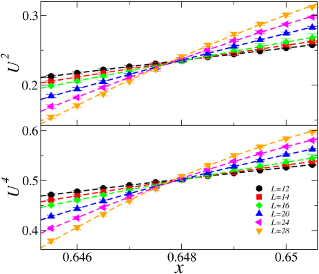
Figure 1: (color online) Curve crossings for the second (upper graph) and fourth (lower graph) order cumulants for various lattice sizes as function of the control parameter $x$. The crossing region is the same in both cases. Dashed lines are third order polynomial fittings.

The estimation of the critical point is shown in Figure 2, where we use the notation $\delta=x_{ij}^{4}-x_{ij}^{2}$ and $\sigma=(x_{ij}^{4}+x_{ij}^{2})/2$. The linear fit gives an estimated for the critical point of $x_{c}=0.64744(14)$ that is in a good agreement with the reported by Yang et al. of $x_{c}=0.646(2)$. Our result improve the previous one by one order of magnitude.

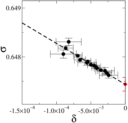
Figure 2: (color online) Evaluation of the critical point using the quantities $\sigma=(x^{4}_{ij}+x^{2}_{ij})/2$ and $\delta=x_{ij}^{4}-x_{ij}^{2}$, where $x^{q}_{ij}$ is the crossing point between cumulants $U^{q}$ for linear sizes $L_{i}$ and $L_{j}$. The dashed line is the linear fit and the red diamond shows the critical point.

The leading correction exponent $\omega$ and the universal quantities $U^{2}_{\infty}$ and $U^{2}_{\infty}$ can be obtained using (15) at the critical point, using a non-linear curve fitting. Our computed values are $\omega=0.6(2)$, $U^{2}_{\infty}=0.207(8)$ and $U^{4}_{\infty}=0.458(12)$. Our results for the cumulants are in good agreement with the reported values $U^{2}=0.2108(7)$ Lundow2010 and $U^{4}=0.4656(4)$ Ballesteros99 of the three-dimensional Ising model. Our result for the $\omega$ exponent is clearly smaller, although within error bar ranges, that previous reported results: $\omega=0.86(9)$ Ballesteros99 , $\omega=0.814(18)$ Guida98 and $\omega=0.782(5)$ Pogorelov2008 ; because of this discrepancy we will evaluate the critical exponents using both our $\omega$ value and a fixed value of $\omega=0.8$, in order to check the validity of our results.

For the evaluation of the critical exponent $\nu$ we use (14) with both cumulants $U^{2}$ and $U^{4}$. Additionally we use the logarithmic derivative of $\langle m\rangle$ and $\langle m^{2}\rangle$, which have the same scaling properties of the cumulant slope Ferrenberg91

$$\frac{\partial\ln\langle m^{n}\rangle}{\partial x}\Bigl{|}_{x=x_{c}}\propto L^{1/\nu}(1+z_{n}L^{-\omega}).$$ (20)

Here the $z_{n}$ are non universal constants. In Figure 3 we are showing the derivatives of the thermodynamic quantities used to evaluate $1/\nu$.

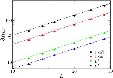
Figure 3: (color online) Log-log plot of several derivatives at the critical point as function of the linear dimension $L$, from top to bottom: $Y(L)=\ln\langle m^{2}\rangle,~{}\ln\langle m\rangle$, $U^{2}$ and $U^{4}$. The dashed lines show the expected power law behavior in the $L\to\infty$ limit with $1/\nu=1.597$.

The results for $1/\nu$ from the fits with two different values of $\omega$ are given in Table 1. We observe that the $U^{2}$ fitting give the largest error of all.

Table 1: Estimates for $1/\nu$ obtained from the fitting of Eqs. (14) and (20) at the critical point $x_{c}=0.64744(14)$.

		$1/\nu$
	$\omega=0.6$		$\omega=0.8$
$U^{2}$	1.617(51)		1.622(43)
$U^{4}$	1.599(12)		1.602(10)
$\ln\langle m\rangle$	1.594(16)		1.603(13)
$\ln\langle m^{2}\rangle$	1.592(20)		1.603(17)

Combining the results we get $1/\nu=1.597(29)$ or $\nu=0.626(11)$ for $\omega=0.6$ and $1/\nu=1.604(24)$ or $\nu=0.623(9)$ for $\omega=0.8$. Both results are in good agreement with the results $\nu=0.6305(5)$, obtained by field theoretical renormalization group method (RG) Pogorelov2008 , and $\nu=0.6302(1)$, obtained by Monte Carlo simulations (MC) Campbell2011 , for the three-dimensional Ising model.

For the critical exponent $\gamma$ we are using Eq. (13) to fit our data at the critical point (see Figure 4). Our results are $\gamma/\nu=1.952(11)$ or $\gamma=1.222(23)$ for $\omega=0.6$ and $\gamma/\nu=1.976(9)$ or $\gamma=1.232(19)$ for $\omega=0.8$. Again the agreement is acceptable compared with the values $\gamma=1.2411(6)$ (RG) Pogorelov2008 and $\gamma=1.2372(4)$ (MC) Campbell2011 .

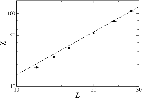
Figure 4: Log-log plot of the susceptibility at the critical point as function of the linear dimension $L$. The dashed lines show the expected power law behavior in the $L\to\infty$ limit with $\gamma/\nu=1.952$.

The fitting for the $\beta$ exponent is shown in Figure 5. Our estimates are $\beta/\nu=0.528(54)$ or $\beta=0.331(34)$ for $\omega=0.6$, and $\beta/\nu=0.521(45)$ or $\beta=0.325(28)$ for $\omega=0.8$. We compare our results with $\beta=0.3253(8)$ (RG) and $\beta=0.3267(2)$, built with the values of $\gamma$ and $\nu$ reported in Pogorelov2008 and Campbell2011 , observing that all results are in good agreement.

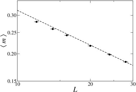
Figure 5: Log-log plot of the order parameter at the critical point as function of the linear dimension $L$. The dashed lines show the expected power law behavior in the $L\to\infty$ limit for $\beta/\nu=0.528$.

One important point of our results is that in both cases the Rushbrooke and Josephson hyperscaling relation is satisfied, we obtain $(\gamma+2\beta)/\nu=3.008(55)$ for $\omega=0.6$ and $(\gamma+2\beta)/\nu=3.012(46)$ for $\omega=0.8$. In Table 2 we summarize the results for the MV model from this work, the values obtained previously by Yang et al., and the known values of the three-dimensional Ising model obtained by Monte Carlo Simulations.

Table 2: Critical values for the MV and the Ising models in three-dimensional lattices.

	This work $(\omega=0.6)$	Yang et al. Yang2008	Ising
$U^{2}_{\infty}$	$0.207(8)$	$-$	$0.2108(7)$ Lundow2010
$U^{4}_{\infty}$	$0.458(12)$	$-$	$0.4656(4)$ Ballesteros99
$\nu$	$0.626(11)$	$0.63(1)$	$0.6302(1)$ Campbell2011
$\gamma$	$1.222(23)$	$1.32(3)$	$1.2372(4)$ Campbell2011
$\beta$	$0.331(34)$	$0.38(1)$	$0.3267(2)$ Campbell2011
$(\gamma+2\beta)/\nu$	$3.008(55)$	$3.30(1)$	$3.0000(12)$ Campbell2011

V Conclusions

The MV model on three-dimensional simple cubic lattices belongs to Ising model universality class. Our simulations prove that the set of critical exponents for both models are consistent when corrections to scaling are included. The incertitude in the value of $\omega$ indicates that it is necessary to increase the simulation data in order to improve the accuracy of the leading correction exponent. However, we have shown that the results are not considerably affected by the choice between $\omega=0.6$ or $\omega=0.8$. In this case the conjecture of Grinstein et al. Grinstein is satisfied, however, we believe that additional numerical simulations in the fourth-dimensional case should be made in the future in order to corroborate the conclusion made by Yang et al. Yang2008 about the critical dimension for the MV model. One open interesting topic is whether or not the dynamical critical phenomena of the MV model is the same that in the Ising model. There are some works that indicate that it is the case for two-dimensional systems Mendes98 ; Tome98 ; Sastre03 , but results for larger dimensionalities are non-existent.

VI Acknowledgments

We wish to thank to G. Pérez for helpful comments and suggestions. A. L. Acuña-Lara thanks Conacyt (México) for fellowship support. This work was supported by Conacyt (México) through Grant No. 61418/2007.

References

- (1) M. J. Oliveira, J. Stat. Phys. 66, 273 (1992).
- (2) W. Kwak, J.-S. Yang, J.-I. Sohn and I.-M. Kim, Phys. Rev. E 75, 061110 (2007).
- (3) G. Grinstein, C. Jayaprakash and Y. He, Phys. Rev.. Lett. 55, 2527 (1985).
- (4) P. R. A. Campos, V. M. de Oliveira and F. G. Brady Moreira, Phys. Rev. E 67, 026104 (2003).
- (5) F. W. S. Lima, U. L. Fulco and R. N. Costa Filho, Phys. Rev. E 71, 036105 (2005).
- (6) F. W. S. Lima and K. Malarz, Int. J. Mod. Phys. C 17, 1273 (2006).
- (7) Z.-X. Wu and P. Holme, Phys. Rev. E 81, 011133 (2010).
- (8) J.-S. Yang, I.-M. Kim and W. Kwak, Phys. Rev. E 77, 051122 (2008).
- (9) M. J. de Oliveira, J. F. F. Mendes and M. A. Santos, J. Phys. A 26, 2317 (1993).
- (10) K. Binder, Z. Phys. B 43 119, (1981).
- (11) H.-P. Deutsch, J. Stat. Phys. 67, 1039 (1992).
- (12) G. Pérez, J. Phys.: Conf. Ser. 23 135 (2005).
- (13) P. H. Lundow and I. A. Campbell, Phys. Rev. B, 82, 024414 (2010).
- (14) H. G. Ballesteros, L. A. Fernandez, V. Martin-Mayor, G. Parisi and J. J. Ruiz-Lorenzo, J. Phys. A 32, 1 (1999).
- (15) R. Guida and J. Zinn-Justin, J. Phys. A 31, 8103 (1998).
- (16) A. A. Pogorelov and I. M. Suslov, JETP 106, 1118 (2008).
- (17) A. M. Ferrenberg and D. P. Landau, Phys. Rev. B, 44, 5081 (1991).
- (18) I. A. Campbell and P. H. Lundow, Phys. Rev. B, 83, 014411 (2010).
- (19) J. F. F. Mendes and M. A. Santos, Phys. Rev. E 57 108, (1998).
- (20) T. Tomé and M. J. de Oliveira, Phys. Rev. E 58, 4242 (1998).
- (21) F. Sastre, I. Dornic and H. Chaté, Phys. Rev. Lett. 91, 267205 (2003).