Dark energy, matter creation and curvature

Abstract

The most studied way to explain the current accelerated expansion of the universe is to assume the existence of dark energy; a new component that fill the universe, does not clumps, currently dominates the evolution, and has a negative pressure. In this work I study an alternative model proposed by Lima et al. lima96 , which does not need an exotic equation of state, but assumes instead the existence of gravitational particle creation. Because this model fits the supernova observations as well as the $\Lambda$CDM model, I perform in this work a thorough study of this model considering an explicit spatial curvature. I found that in this scenario we can alleviate the cosmic coincidence problem, basically showing that these two components, dark matter and dark energy, are of the same nature, but they act at different scales. I also shown the inadequacy of some particle creation models, and also I study a previously propose new model that overcome these difficulties.

I Introduction

Currently the observational evidence coming from supernovae studies SNIa , cosmic background radiation fluctuations cmbr , and baryon acoustic oscillations bao , set a strong case for a cosmological (concordance) universe model composed by nearly $70$ percent of a mysterious component called dark energy, responsible for the current accelerated expansion, nearly $25$ percent of dark matter, which populates the galaxy halos and a small percentage (around $4$) is composed by baryonic matter. The nature of these two dark component remains so far obscure DEDM . In the case of dark matter, we have a set of candidates to be probed with observations and detections in particle accelerators, however the case of dark energy is more elusive. This component not only has to fill the universe at the largest scale homogeneously, and also has the appropriate order of magnitude to be comparable to dark matter, but also has to have a negative pressure equation of state, something that was assumed first to explain inflation in the early universe, inspired by high energy theories of particle physics, but which seems to be awkward to appeal for, at these low energy scales. The alternative way to account for the cosmic acceleration, in the framework of the standard model, is to consider a modification of general relativity at large scales alterGR .

Some years ago, Prigogine and co-workers prigogine presented a very interesting cosmological model where matter creation takes place without spoiling adiabatic expansion. This is possible by adding a work term due to the change of the particle number density $n$. This work actually suggested for the first time, a way to incorporate the particle creation process in the context of cosmology in a self consistent way. In fact, the original claim made by Zeldovich zeldov70 , that gravitational particle production can be described phenomenologically by a negative pressure, is realize here in a beautiful way. A covariant formulation of the model was presented for the first time in CLW90 .

Originally, these considerations were applied in the context of; the steady-state cosmological model, the warm inflationary scenario and within the standard inflationary scenario, during the reheating phase. Based on this work, the studies of cosmological models with matter creation lima96 were initiated, and rapidly recognized to be potentially important to explain dark energy harko . In particular, in Ref.zsbp01 the authors established a model where dark energy can be mimicked by self-interactions of the dark matter substratum. Within the same framework, models of interacting dark energy and dark matter were proposed interact . Actually, in these studies is possible to have consistently, a universe where matter creation proceeds within an adiabatic evolution. More recently, Lima et al.,lima08 have presented a study of a flat cosmological model where a transition from decelerated to accelerated phase exist. They explicitly show that previous models considered lima99 , does not exhibit the transition, and study the observational constraints on the model parameters. Also in Steigman:2008bc the authors modified slightly the model, adding explicitly a baryonic contribution, which enable them to have a transition from decelerated to accelerated expansion always.

In this work I consider the non flat extension of this matter creation cosmological model. This is important because, even in the $\Lambda$CDM concordance model, there is no clear evidence that $\Omega_{k}$ is zero, due to the well known degeneracy between $w(z)$ and $\Omega_{k}$ curvature . Furthermore, any alternative model to dark energy then must consider a non flat assumption as a prior. This model enable us to explain the current acceleration of the universe expansion through a fictitious pressure component coming from changes in the dark matter particle number, without any exotic contribution. As a bonus, this model enable us to explain easily the cosmic coincidence problem; it is not strange to have a similar contribution from these two (commonly differently regarded) components, because they are just two aspects of one and the same component; the dark matter.

In the next section I derive the equations of motion in the case of matter creation. Then, in section III I study the case for non flat models and the observational consequences in the models already knew. After this, I discuss a new particle creation model that resembles the $\Lambda$CDM model case, showing the transition from a decelerated to an accelerated expansion without enter in conflict with the behavior for large z.

II The effective negative pressure

Assuming that the particle number is not conserved $N^{\mu}_{;\mu}\neq 0$, it leads to a modification of the energy conservation equation. In fact, assuming $N^{\mu}_{;\mu}=n\Gamma$ where $\Gamma$ is the particle creation rate, and using the FRW metric we obtain the generalization of the energy conservation equation,

$$d(\rho V)+pdV-(h/n)d(nV)=0,$$ (1)

where $h=(\rho+p)$ is the enthalpy (per unit volume), $n$ is the number density and $\rho$ is the energy density, and a new equation

$$\dot{n}+3Hn=n\Gamma,$$ (2)

for the non conserved number density. The important thing to stress here is that the universe evolution continues to be adiabatic, in the sense that the entropy per particle remains unchanged ($\dot{s}=0$). The extra contribution can be interpreted in (1) as a non thermal pressure defined as

$$p_{c}=-\left(\frac{\rho+p}{3H}\right)\Gamma.$$ (3)

This is the source that produces the acceleration of the universe expansion. Once the particle number increases with the volume, we obtain a negative pressure.

Now, because we are considering matter creation, we have to impose the second law constraint

$$dS=\frac{s}{n}d(nV)\geq 0,$$ (4)

where $s=S/V$ is the entropy density. From (1) we find that the new set of Einstein equations are

$$H^{2}+\frac{k}{R^{2}}=\frac{8\pi G}{3}\rho$$ (5)

$$\dot{\rho}=\frac{\dot{n}}{n}(\rho+p)$$ (6)

and the previously derived relation (2). The set of equations (2), (5) and (6) completely specified the system evolution. It is also useful to combine (3) with (5) and (6) to eliminate $\rho$ and obtain

$$2\frac{\ddot{R}}{R}+\frac{\dot{R}^{2}}{R^{2}}+\frac{k}{R^{2}}=-8\pi G(p+p_{c}).$$ (7)

The standard adiabatic evolution is easily recovered: setting $\Gamma=0$ implies that $\dot{n}/n=-3H$, which leads to the usual conservation equation from (6). A class of de Sitter solution is obtained with $\dot{n}=\dot{\rho}=0$ and arbitrary pressure $p$. Moreover, there exist another class of solutions where Eq.(6) enable us to determine the pressure; for example if $\rho=mn$, with $m$ constant, Eq.(6) implies $p=0$, and furthermore if $\rho=aT^{4}$ and $n=bT^{3}$ implies $p=\rho/3$.

I have to stress here that the main result derived in this section means that we have a single contribution, which satisfy the non-relativistic matter equation of state, that describe both dark matter and dark energy simultaneously, and in this way solves automatically the coincidence problem. This dark unification mechanism does not have the problem studied in STZW , because in the cases studied in that paper, for example the Chaplygin gas model chaplygin , the sound velocity of the dark matter is not zero, leading to instabilities. That happens because the Chaplygin gas interpolates between the equation of states for dark matter and dark energy. This does not happens here, because there is just one equation of state; that of non-relativistic matter.

III Matter creation in a non flat universe

In this section we study a number of models where matter creation produces cosmic acceleration, in a curved background. We also test the models using the most recent Supernovae data, the so called Union 2 set Union2 . In order to do that test we consider the comoving distance from the observer to redshift $z$ is given by

$$r(z)=\frac{1}{\sqrt{-\Omega_{k}}}\sin\sqrt{-\Omega_{k}}\int_{0}^{z}\frac{dz^{\prime}}{E(z^{\prime})},$$ (8)

where $E(z)\equiv H(z)/H_{0}$. The SNIa data give the distance modulus $\mu(z)$ which is related to the luminosity distance $d_{L}(z)=(1+z)r(z)$, through $\mu(z)\equiv 5\log_{10}[d_{L}(z)/\texttt{Mpc}]+25$. We fit the SNIa with the cosmological model by minimizing the $\chi^{2}$ value defined by

$$\chi_{SNIa}^{2}=\sum_{i=1}^{557}\frac{[\mu(z_{i})-\mu_{obs}(z_{i})]^{2}}{\sigma_{\mu i}^{2}},$$ (9)

where $\mu_{obs}$ is the corresponding observed one.

III.1 $\beta$ Model

Let us assume first the particle creation rate evolving as

$$\Gamma=3H\beta,$$ (10)

where $\beta$ is a constant. From (2) we finds the solution for the density number

$$n(R)=n_{0}\left(\frac{R_{0}}{R}\right)^{3(1-\beta)},$$ (11)

where $n_{0}$ is a constant of integration. Assuming $\rho=mn$ as for non-relativistic matter (that leads to que usual equation of state $p=0$ as we discussed that at the end of the last section), we get for the Hubble function

$$E^{2}(z)=\Omega_{m}(1+z)^{3(1-\beta)}+(1-\Omega_{m})(1+z)^{2}.$$ (12)

Clearly, this model does not describe properly a transition from decelerated to an accelerated expansion phase. In fact, from (5) and (6) we obtain:

$$\frac{\ddot{R}}{R}=4\pi G\rho\left(\beta-\frac{1}{3}\right).$$ (13)

Depending on the value assumed for $\beta$ we obtain a model that accelerate forever ($\beta>1/3$) or decelerate forever ($\beta<1/3$).

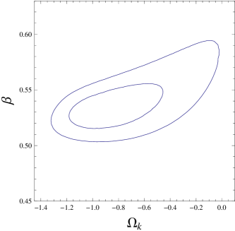
Figure 1: Using the Union 2 data set Union2 we plot the confidence contours, at $68.27\%$ and $95.45\%$ for the two parameters of the model: $\beta$ and $\Omega_{k}$.

A Bayesian analysis using the Union 2 data set of SNIa Union2 enable us to plot confidence contours for the two parameters of the model: $\beta$ and $\Omega_{k}$. This is shown in Fig.1. Clearly, the data suggest a large negative value for the curvature parameter, indicating that in order to fit the SNIa data, the function $H(z)$ has to have a very distorted form. In any case, because this model does not present a transition from a decelerated to an accelerated phase, it can be ruled out immediately.

III.2 $\gamma$ model

As is well known from observations of supernovae, a transition from a decelerated to an accelerated expansion occurs in the recent history of the universe. Depending on what is used to model dark energy, different redshift have been obtained between $0.5$ to $1$. In the context of a model of adiabatic matter creation, this topic was recently discussed in lima08 where the authors specialized in a flat cosmology, where a explicit transition can be achieved from a decelerated to an accelerated expansion using the following model

$$\Gamma=3\gamma H_{0}.$$ (14)

In this section we generalize this work to non flat universes. In what follows, a non relativistic matter equation of state is assumed $\rho=mn$ ($p=0$).

Introducing (14) in (2) leads to the following solution

$$n(R)=n_{0}\left(\frac{R_{0}}{R}\right)^{3}e^{3H_{0}\gamma(t-t_{0})}.$$ (15)

Is evident the meaning of the subscript zero. Because $\rho=mn$ for non-relativistic matter and using (7) we obtain

$$\frac{\ddot{R}}{R}=4\pi G\left(\gamma\frac{H_{0}}{H}-\frac{1}{3}\right),$$ (16)

that clearly allow us to describe an acceleration/deceleration transition. Writing the right hand side in terms of $H$ and using the Hubble equation once more, we can write

$$\dot{H}+H^{2}=\frac{3}{2}\left(H^{2}+\frac{k}{R^{2}}\right)\left(\gamma\frac{H_{0}}{H}-\frac{1}{3}\right).$$ (17)

For $k=0$ this equation coincides with that in lima08 , for which an explicit form of $H(z)$ was found. In the general case, $k\neq 0$, it is not possible to integrate (17) to obtain a closed analytic form. Instead, we use $\dot{R}/R=H$ to change the time derivatives for derivatives of the scale factor $R$, and using that $R_{0}/R=1+z$, change again the derivatives in terms of the redshift. Doing that, we obtain

$$(1+z)E\frac{dE}{dz}-E^{2}=\left[\Omega_{k}(1+z)^{2}-E^{2}\right]\left(\frac{3\gamma}{2E}-\frac{1}{2}\right),$$ (18)

where $E(z)=H(z)/H_{0}$. Given the set of parameters $\Omega_{k}$ and $\gamma$, we integrate numerically (18) to obtain the function $E(z)$.

Figure 2: Using the Union 2 data set Union2 we plot the confidence contours, at $68.27\%$ and $95.45\%$ for the two parameters of the model: $\gamma$ and $\Omega_{k}$, by integrating Eq. (18).

A Bayesian analysis using the Union 2 data set of SNIa Union2 enable us to plot confidence contours for the two parameters of the model: $\gamma$ and $\Omega_{k}$. This is shown in Fig.2. Again, as in the previous subsection, the SNIa data suggest a very large negative value for $\Omega_{k}$.

III.3 Problems with these models

A simple way to understand the large negative values obtained for $\Omega_{k}$ in the fitting process, which is suggested by the SNIa data in these models, is by plotting the $H(z)$ function in the range $z\in(0,4)$. In Fig. 3 we display such a plot.

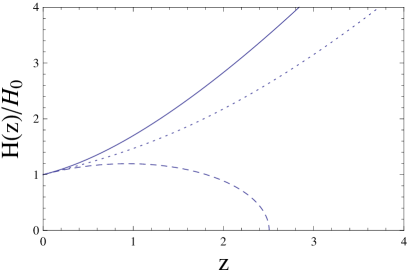
Figure 3: The Hubble function in terms of the redshift for the $\beta$ model (dashed line), the $\gamma$ model (dotted line) and the flat LCDM model, $(\Omega_{m},\Omega_{\Lambda})=(0.27,0.73)$ (continuos line).

All the three models have two free parameters to be fixed with the SNIa data. Although at low redshift ($z<0.2$) the three curves coincide, their evolution with increasing $z$ differs appreciably. Clearly the $\beta$ model behaves erroneously. Instead, the $\gamma$ model, although it has the correct tendency, it is easily differentiated from the LCDM at large redshift ($z>0.2$). Because we are using the SNIa data set, the best fit values for the free parameters in these models (shown in Fig.3) adjust principally the low-$z$ zone, because from the $557$ SNIa data only $19$ have $z>1$. This is also clear once we try to perform a joint Bayesian analysis using SNIa plus the BAO and CMB constraints (see Table I). Using the $\beta$ model, the procedure even does not find any appropriate configuration. Using the $\gamma$ model, it is possible to get a good fit ($\chi_{red}=0.994$) using only SNIa+BAO, however once we add the CMB constraint, it worsens the fit ($\chi_{red}=1.32$).

Table 1: The $\chi^{2}$ for the best fit values in models discussed in this section plus the curved $\Lambda$CDM using the Union2 data set in the case of a non flat universe model.

Model	SN	SN+BAO	SN+BAO+CMB
$\beta$ Model	542.17	554.99	—
$\gamma$ Model	542.29	552.66	731.12
$\Lambda$CDMk	542.55	542.65	542.65

It is therefore clear why in Steigman:2008bc the authors add an explicit contribution for baryons. Adding baryonic dark matter with $\Omega_{B}=0.042$ in the previous models, enable us to obtain better best fit parameters for the models that, for instance modifying Fig. 3 into Fig. 4.

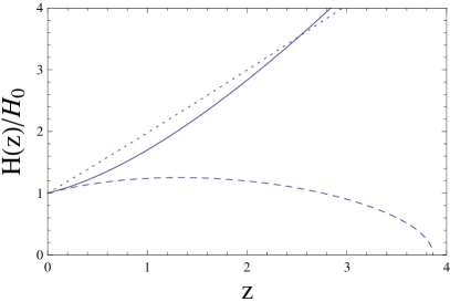
Figure 4: The same as Fig. 3, but this time considering baryonic dark matter with $\Omega_{B}=0.042$. See the text for a discussion.

For example, in the case of the $\gamma$ model, once we add baryons the best fit parameters improve respect to the case without baryons; using only SNIa+BAO we get a $\chi_{red}=0.989$, however once we add the CMB constraint, it worsens the fit again.

IV Search for a New model

The previous models have been discussed in several papers, deriving their consequences in cosmological evolution and also testing their performance to fit the supernova data. The problem with the $\beta$ model is that it can not describe properly a transition from a decelerated to an accelerated phase. In contrast, the $\gamma$ model can do this, however they can only fit well low-redshift observational constraint (SNIa data with $z<0.2$). As we mentioned in the last section, if we attempt to include the BAO and CMB constraint, the whole fit breaks down.

The objective merit of this type of model is that we can mimic a cosmological constant without use of an exotic component, we just need to assume the existence of matter creation that takes place with a certain rate. In principle, we do not have any fundamental reason to use a specific form of the matter creation rate. The only fundamental feature we have to respect is the second law of thermodynamics (4).

In Cardenas:2008zv we propose a model that was also discussed in Lima:2009ic . Let us consider this model here as an example. This model is characterized by the following matter creation rate

$$n\Gamma=3\alpha H,$$ (19)

which for $\alpha>0$ satisfy the requirement, because $H(z)$ is a positive definite function. Inserting in (2) we obtain

$$n(R)=(n_{0}-\alpha)\frac{R_{0}^{3}}{R^{3}}+\alpha.$$ (20)

that resembles the combined contribution of a cosmological constant and dust. The level of fine tuning here to obtain an accelerated expansion is relatively smaller than in the usual $\Lambda$CDM model, because in this case, both terms come from the same function, and we know that we can obtain an accelerated expansion phase after some period of time from (5). In fact, from (3) we get $p_{c}=-m\alpha$, so replacing in (7) we find

$$\frac{\ddot{R}}{R}=\frac{4\pi Gm}{3}\left[2\alpha-(n_{0}-\alpha)\left(\frac{R_{0}}{R}\right)^{3}\right].$$ (21)

Note however that the equation of state has not been modified, $\rho$ is still the non-relativistic contribution. We do not have to introduce any exotic component - with a negative pressure - to describe the current expansion acceleration. Given the current status of the dark matter and dark energy problem DEDM , we can use this idea as a possible way to understand it. Replacing in the Hubble equation we obtain

$$E(z)^{2}=\Omega_{\alpha}+(1-\Omega_{\alpha}-\Omega_{k})(1+z)^{3}+\Omega_{k}(1+z)^{2},$$ (22)

where $\Omega_{\alpha}=m\alpha/\rho_{cr}$ and $\rho_{cr}=3H_{0}^{2}/8\pi G$, which is effectively indistinguishable from a curved LCDM model. Because $\Omega_{\alpha}=\Omega_{\Lambda}=0.7$, is clear that the observations implies a positive $\alpha$ for this new model.

In this work I have studied a model which considering small changes in the total number of particles in our universe, offer a possible way to understand the current accelerated expansion measurements, without using any exotic energy component. Also, this scenario alleviate the cosmic coincidence problem, basically showing that these two components, dark matter and dark energy, are of the same nature, but their act at different scales. This way of understand the SNIa observations, implies that cosmology have a new window to explore the universe considering matter creation, encoded in the function $dN/dV$. I have discussed the two models already known in the literature, extending the analysis to nonflat universes, performing a bayesian analysis using both SNIa and also BAO and CMB. I have found that, both the $\beta$ and $\gamma$ models fail to fit the observations, even considering $\Omega_{k}\neq 0$. Although adding an explicit baryonic dark matter contribution may ameliorate the fit using SNIa+BAO in the $\gamma$ model, adding the CMB constraint worsens the situation. The statistical analysis was performed even in the case an explicit form for $H(z)$ was lacking. I have also studied a previously proposed new model, through a specific form of the matter creation rate, which is almost indistinguishable from a LCDM model, which enable us to fit all the observations, SNIa+BAO+CMB. Although similar to LCDM, the model can be distinguished through the structure formation process, which will be studied elsewhere.

References

- (1) A. Riess et al., Astrophys. J. 607, 665 (2004); J.L. Tonry et al., Astrophys. J. 594, 1 (2003).
- (2) D.J. Eisenstein et al., Astrophys. J. 633, 560 (2005).
- (3) D.N. Spergel et al., Astrophys. J. Suppl. 170, 377 (2007).
- (4) J.A. Frieman, M.S. Turner and D. Huterer, arXiv: astro-ph/0803.0982; M. Taoso, G. Bertone and A. Masiero, arXiv: astro-ph/0711.4996; D. Hooper and E.A. Baltz, Annu. Rev. Nucl. Part. Sci. 58, (2008)(arXiv: hep-ph/0802.0702).
- (5) S.M. Carroll, V. Duvvuri, M. Trodden and M.S. Turner, Phys. Rev. D 70, 043528 (2004); S. Capozziello, “Dark energy and dark matter as curvature effects”, to be published in the Proceedings of the 11th Marcel Grossmann Meetng, Berlin, July (2006).
- (6) I. Prigogine, J. Geheniau, E. Gunzig and P. Nardone, Proc. Natl. Acad. Sci. USA, Vol 85, 7428 (1988); ibid, Gen. Rel. Grav. 21, 767 (1989).
- (7) Ya. B. Zeldovich, JETP Lett. 12, 307 (1970).
- (8) J.A. Lima, M.O. Calvao and I. Waga, Frontier Physics, Essays in Honor of Jayme Tiomno, World Scientific, 1991, arXiv: astro-ph/0708.3397.
- (9) L.R.W. Abramo and J.A.S. Lima, Class. Quant. Grav. 13, 2953 (1996); W. Zimdahl, Phys. Rev. D 53, 5483 (1996); W. Zimdahl and D. Pavón, Mon. Not. R. Astron. Soc. 266, 872 (1994).
- (10) W. Zimdahl, Phys. Rev. D 61, 083511 (2000); M.K. Mak and T. Harko, Aust. J. Phys. 52, 659 (1999).
- (11) W. Zimdahl, D.J. Schwarz, A.B. Balakin and D. Pavon, Phys. Rev. D 64, 063501 (2001).
- (12) L. Amendola, S. Tsujikawa and M. Sami, Phys. Lett. B 632, 155 (2006); L. Amendola and C. Quercellini, Phys. Rev. D 68, 023514 (2003); L.P.Chimento, A.S. Jakubi, D. Pavon and W. Zimdahl, Phys. Rev. D 67, 083513 (2003); W. Zimdahl and D. Pavon, Phys. Lett. B 521, 133 (2001); L. Amendola, Phys. Rev. D 62, 043511 (2000).
- (13) J.A.S. Lima, F.E. Silva and R.C. Santos, Class. Quant. Grav. 25, 205006 (2008).
- (14) J.A.S. Lima and J.S. Alcaniz, Astron. Astrophys. 348, 1 (1999); J.S. Alcaniz and J.A.S. Lima, Astron. Astrophys. 349, 729 (1999).
- (15) G. Steigman, R. C. Santos and J. A. S. Lima, JCAP 0906, 033 (2009) [arXiv:0812.3912 [astro-ph]].
- (16) A. Shafieloo and E. V. Linder, Phys. Rev. D 84, 063519 (2011) [arXiv:1107.1033 [astro-ph.CO]]; P. M. Okouma, Y. Fantaye and B. A. Bassett, arXiv:1207.3000 [astro-ph.CO].
- (17) V. H. Cardenas, arXiv:0812.3865 [astro-ph].
- (18) J. A. S. Lima, J. F. Jesus and F. A. Oliveira, JCAP 1011, 027 (2010) [arXiv:0911.5727 [astro-ph.CO]].
- (19) S. Basilakos and J. A. S. Lima, Phys. Rev. D 82, 023504 (2010) [arXiv:1003.5754 [astro-ph.CO]].
- (20) H.B. Sandvik, M. Tegmark, M. Zaldarriaga and I. Waga, Phys. Rev. D 69, 123524 (2004); R. Bean and O. Dore, Phys. Rev. D 68, 023515 (2003).
- (21) A. Kamenshchik, U. Moschella and V. Pasquier, Phys. Lett. B 511, 265 (2001); M.C. Bento, O. Bertolami, A.A. Sen, Phys. Rev. D 67, 063003 (2003).
- (22) R. Amanullah et al., Astrophys. J. 716, 712 (2010) [arXiv:1004.1711 [astro-ph.CO]].