The Age-Redshift Relation For Luminous Red Galaxies obtained from the Full Spectrum Fitting and its cosmological implications

Abstract

The relative age of galaxies at different redshifts can be used to infer the Hubble parameter and put constraints on cosmological models. We select luminous red galaxies (LRGs) from the SDSS DR7 and then cross-match it with the MPA/JHU catalogue of galaxies to obtain a large sample of quiescent LRGs at redshift $z\sim 0.03-0.39$. The total 23,883 quiescent LRGs are divided into four sub-samples according to their velocity dispersions and each sub-sample is further divided into 12 redshift bins. The spectra of the LRGs in each redshift and velocity bin are co-added in order to obtain a combined spectrum with relatively high $S/N$. Adopting the GalexEV/SteLib model, we estimate the mean ages of the LRGs from these combined spectra by the full-spectrum fitting method. We check the reliability of the estimated age by using Monte-Carlo simulations and find that the estimates are robust and reliable. Assuming that the LRGs in each sub-sample and each redshift bin were on average formed at the same time, the Hubble parameter at the present time $H_{0}$ is estimated from the age–redshift relation obtained for each sub-sample, which is compatible with the $H_{0}$ value measured by other methods. We demonstrate that a systematic bias (up to $\sim 20\%$) may be introduced to the $H_{0}$ estimation because of recent star formation in the LRGs due to the later major mergers at $z\lesssim 0.4$, but this bias may be negligible for those sub-samples with large velocity dispersions. Using the age–redshift relations obtained from the sub-sample with the largest velocity dispersion or the two sub-samples with high velocity dispersions, we find $H_{0}=65^{+7}_{-3}\rm km~{}s^{-1}~{}Mpc^{-1}$ or $H_{0}=74^{+5}_{-4}\rm km~{}s^{-1}~{}Mpc^{-1}$ by assuming a spatially flat $\Lambda$CDM cosmology. With upcoming surveys, such as the Baryon Oscillation Spectroscopic Survey (BOSS), even larger samples of quiescent massive LRGs may be obtained, and thus the Hubble parameter can be measured with high accuracy through the age–redshift relation.

1. Introduction

The expansion history of the universe are presently studied with a few observational probes, such as the supernova Ia, baryon acoustic oscillations (BAO), weak gravitational lensing, and galaxy clusters, etc. Each of these probes has its pros and cons, and suffer from different systematic uncertainties (e.g., Freedman & Madore, 2010). A new observational probe of the cosmic expansion history would be invaluable, and can provide additional cross check with the results obtained from the existing methods. Combining the results obtained by different means may further help to constrain robustly the dynamical nature of the universe.

Jimenez & Loeb (2002) proposed a novel approach to explore the expansion history of the universe, which is based on the age–redshift relation of passively evolving massive galaxies. Assuming that the passively evolving galaxies at different redshifts were born approximately at the same time, the age of these galaxies can then be taken as a cosmic chronometer. If the ages of such galaxies can be accurately estimated, then this age–redshift relation may be used to determine the cosmic expansion history. Even if there is some systematic errors in the absolute age measurements, it is argued that such errors could be canceled in the relative age of these galaxies at different redshifts, thus providing a good measurement of $H(z)$:

$$H(z)=-\frac{1}{1+z}\frac{dz}{dt}.$$ (1)

Indeed, observations show that the most massive galaxies are mainly composed of old stellar populations formed at redshifts $z>1-2$, less than $1\%$ of their present stellar mass is formed at $z<1$ (Dunlop et al., 1996; Spinrad et al., 1997; Cowie et al., 1999; Heavens et al., 2004; Thomas et al., 2005; Cimatti et al., 2008; Thomas et al., 2010), hence these galaxies are suitable for this application.

Jimenez et al. (2003) applied this method to a sample of massive galaxies at low redshift by fitting their spectra with the single stellar population (SSP) spectra based on the SPEED model (Jimenez et al., 2004), and obtained $H_{0}=69\pm~{}12\rm km~{}s^{-1}~{}Mpc^{-1}$. Simon et al. (2005) assembled a high redshift data set obtained from the Gemini Deep Survey (GDDS) and some other archival data, and applied the same method to estimate $H(z)$ for a large redshift range ($z\sim 0.1-1.8$). These earlier works on the age–redshift relation adopted the SSP to fit each galaxy spectrum in the sample, and selected the age of the oldest one in each redshift bin as the envelop of the age. However, the poor signal-to-noise ratio ($S/N$) spectra of individual galaxies and the contamination from the telluric emission and absorption may lead to uncertainties in the age estimates, and the method of the oldest galaxy envelop draw results from a small number of galaxies at the extremes of the distribution, which may also undermine the validity of the result, and makes the method hard to use.

To overcome this problem, Carson & Nichol (2010) obtained the combined spectra for those luminous red galaxies (LRGs) with similar physical properties in each redshift bin by co-adding their spectra, of which the $S/N$ is much higher than individual galaxies. They then estimated the age of the combined spectra by using the standard Lick absorption line indices, which may be regarded as the mean age of a large sample of galaxies. They obtained the age–redshift relation, but they did not use this relation to further constrain the Hubble parameter.

In this paper, we first select a LRG sample from the SDSS data release 7 (DR7). In order to improve the $S/N$ and remove the contamination, we also use the combined spectrum rather than the single spectrum of each galaxy. However, we adopt the full spectrum fitting method, different from the standard Lick absorption line indices adopted by Carson & Nichol (2010), to estimate the mean age of the combined spectrum, and then obtain the age–redshift relation. Furthermore, we also use the age-redshift relation obtained from the combined spectra to constrain the Hubble parameter at the present time $H_{0}$ and analyze the possible systematic bias in the estimated $H_{0}$. The paper is organized as follows. In Section 2, we describe the selection criteria of the LRG sample. In Section 3, we provide the details of the fitting method and the age–redshift relation estimated from the LRG sample. In Section 4, we constrain the Hubble parameter by using the obtained age-redshift relation. Discussions on the resulted age–redshift relation and the possible associated systematic bias are given in Section 5. Conclusions are summarized in Section 6.

2. Sample selection

In order to obtain the age–redshift relation and use it to measure the Hubble parameter, it is necessary to first select a large sample of passively evolving galaxies that contains the oldest populations with homogeneous physical properties. The SDSS is currently the largest survey that provides hundreds of millions of detected objects with accurate photometric and astrometric calibrations, and part of the objects have excellent spectra (Pier et al., 2003; Hogg et al., 2001). It is generally accepted that the LRGs are passively evolving galaxies and that they host the oldest stellar populations. Therefore, we pick our sample from the LRGs of the SDSS DR7 (York et al., 2000; Abazajian et al., 2009).

For our purpose, it is necessary to determine the physical properties of the LRGs with relatively high accuracy by using their spectra. Considering that some physical parameters such as the velocity dispersions and emission lines are available in the MPA/JHU sample only for CUT I LRGs (see Eisenstein et al., 2001), we select only from the CUT I LRGs. To obtain accurate estimates of the age through the full spectrum fitting method, the selected galaxies should also have sufficiently high $S/N$. Our selection criteria for LRGs are similar to that described in Carson & Nichol (2010), but with an additional restriction on the $S/N$ as follows:

• selecting galaxies from Catalog Archive Server (CAS) database using the TARGET_GALAXY_RED flag;

• selecting galaxies with $S/N>10$ per pixel (in the continuum of the r-band wavelength range);

• selecting galaxies which further satisfying the restrictions: specClass EQ ‘SPEC_GALAXY’,zStat EQ ‘XCORR_HIC’, zWarning EQ 0 , eClass < 0, z < 0.4 and fracDev_r > 0.8 (see more details in Carson & Nichol, 2010).

Figure 1.— The redshift distribution of LRGs. The solid histogram represents the distribution of LRGs in our final sample and the dotted histogram represents the distribution of all LRGs in our paper whose the lower-redshift peak is mostly contributed by the spiral bulges.

According to the criteria above, 71,971 LRGs are selected from the SDSS DR7 and their redshift distribution is shown in Figure 1 (the dotted histogram). These LRGs are probably contaminated by the bulges of late-type galaxies at low redshift, due to the limited fiber size (3″) of the SDSS spectrograph. Such late contaminants would however have new star formations, and it is well known that the [Oii] and $H_{\alpha}$ lines are indicators of star formation, hence we can remove the spiral bulges from the selected sample and obtain an sample of quiescent LRGs by using the spectral line data. Here we use the MPA/JHU spectral line data, which has been widely used in selecting quiescent galaxies in the literature. We select those LRGs as quiescent only if their $H_{\alpha}$ and [Oii] line emission are consistent with zero at $2\sigma$ level. With this criterion, we obtain 27,208 quiescent LRGs. We note here that using other emission lines to select quiescent galaxies may result in a similar quiescent LRG sample, as Carson & Nichol (2010) pointed out that all other emission lines (such as the joint constraint of $H_{\beta}$ and [Oiii] or Nii and Sii) show similar zero-emission line distributions.

To estimate the Hubble expansion rate $H(z)$ by using the age-redshift relation, it is important to select samples of galaxies with homogeneous physical properties as demonstrated by Crawford et al. (2010). For this reason, the quiescent LRGs selected above are divided into four sub-samples according to their velocity dispersions, which are listed in the MPA/JHU galaxy catalog. The velocity dispersion bins for each sub-sample of the LRGs are $200\rm km~{}s^{-1}-230\rm km~{}s^{-1}$, $230\rm km~{}s^{-1}-260\rm km~{}s^{-1}$, $260\rm km~{}s^{-1}-290\rm km~{}s^{-1}$ and $290\rm km~{}s^{-1}-320\rm km~{}s^{-1}$, respectively. We denote these four sub-samples as sub-sample I, sub-sample II, sub-sample III, and sub-sample IV, respectively. In each of the velocity dispersion bins, the number of galaxies is still sufficiently large for the following co-adding spectra to reach a high $S/N$ ($>40$). We do not consider galaxies with velocity dispersions larger than $320\rm km~{}s^{-1}$, as the total number of those galaxies at $z<0.14$ is too small ($<30$). In addition since the total number of galaxies with velocity dispersion less than $200\rm km~{}s^{-1}$ is 1843, much smaller than the number of galaxies in all other sub samples, we also exclude these galaxies. The number of galaxies in each sub-sample is listed in Table 1, and after excluding those LRGs with $\sigma_{v}>320\rm km~{}s^{-1}$ or $\sigma_{v}<200\rm km~{}s^{-1}$, the total number of the final sample is 23,883. The redshift distribution of these galaxies is shown in Figure 1 (the solid histogram).

Table 1The total number of galaxies in each sub-sample.

Sample	Velocity Dispersion Range	Number
sub-sample I	$200\rm km~{}s^{-1}<\sigma_{v}\leq 230\rm km~{}s^{-1}$	$4756$
sub-sample II	$230\rm km~{}s^{-1}<\sigma_{v}\leq 260\rm km~{}s^{-1}$	$8748$
sub-sample III	$260\rm km~{}s^{-1}<\sigma_{v}\leq 290\rm km~{}s^{-1}$	$7149$
sub-sample IV	$290\rm km~{}s^{-1}<\sigma_{v}\leq 320\rm km~{}s^{-1}$	$3230$
total	$200\rm km~{}s^{-1}<\sigma_{v}\leq 320\rm km~{}s^{-1}$	$23,883$

3. Spectral fitting methods

There are three commonly adopted methods for measuring the age and metallicity of a stellar system from its spectrum: (1) the SED fitting, (2) the Lick indices fitting, and (3) the full spectrum fitting. The first method is only sensitive to the general shape of the continuum, the second one focuses on using the strength or equivalent width of lines and specific spectrum features, and the third one accounts all the information of the spectrum, including both the continuum and the lines and specific features. The full spectrum fitting method has several advantages, such as being insensitive to extinction or flux calibration errors, and it is also not limited by the physical broadening of lines since the internal kinematics is determined simultaneously with the population parameters (Koleva et al., 2008), though it is insensitive to the element ratio effects because of yet no available models about these. On the other hand, it is more sensitive to the wavelength range of the spectrum adopted in the fitting and the resolution of the spectrum compared with the fitting with the Lick indices.

3.1. The ULySS software

ULySS is an open-source software package developed by a group in Université de Lyon, which implements the full-spectrum fitting to study physical properties of stellar populations. In ULySS, an observed spectrum is fitted by a model spectrum, adopting a linear combination of non-linear components, optionally convolved with a line-of-sight velocity distribution (LOSVD) and multiplied by a polynomial function. The multiplicative polynomial is adopted to absorb errors of the flux calibration, Galactic extinction and other factors which may affect the shape of the spectrum. It minimizes $\chi^{2}$ value by the MPFIT function when matching an observed spectrum with the model ones. The line spread function (LSF), an analogy to the point spread function (PSF) for images, is also introduced in ULySS in order to effectively match the resolution of the model spectrum to the observations. For details about ULySS, the readers are referred to Koleva et al. (2009a). Since the full spectrum fitting method may be sensitive to the wavelength range of the spectrum adopted in the fitting, we adopt the GalexEV/SteLib model, a popular single stellar populations (SSPs) synthesis model which covers the largest wavelength range, i.e. $3200$Å$-9500$Å. This wavelength range includes the Caii triplet ($\lambda\lambda 8498,8542,8662$Å), which is a prominent feature produced primarily by an old population of red-giants and thus important for determining the age of the quiescent LRGs (Diaz et al., 1989).

The GalexEV/SteLib(GS) population model is produced by the isochrone synthesis code of BC03 (Bruzual & Charlot, 2003), which is widely used in SDSS data analysis. It use the SteLib library which contains 249 spectra, but only 187 stars have measured metallicity and can be used to compute the predicted spectra with a 3Åspectral resolution. The GS model adopts the Padova 94 isochrones (Bertelli et al., 1994) and the Chabrier IMF (Chabrier & Gilles, 2003). Totally 696 SSPs, covering the age of $0.1\sim 20$ Gyr and the [Fe/H] of $-2.3\sim 0.4$ dex, are included in the GS model. The relevant information of the GS model is given in Table 2.

Table 2The settings in the GS model.

Model	Library	Resolution	Wavelength	Age	Z	IMF	Track
		(Å)	(Å)	(Gyr)	(dex)
GS	SteLib	3	3200-9500	0.1-20	$-2.3$-0.4	Chabrier	Padova 94

3.2. Model pre-treatment

The resolution match is a key issue in the model fitting because the resolution of a model spectrum is usually different from that of the observational data. It is necessary to transform either the model spectrum or the observed spectrum to match the resolution of the other one. The spectral resolution is characterized by the instrumental broadening or the LSF. In practice, the LSF is not necessarily a Gaussian and may vary with wavelength (see more details on the LSF in Koleva et al. (2008, 2009a)). In ULySS, three types of calibrations (arc lamp, standard star, twilight spectrum) can be used to determine the relative LSF between the model and the observation. In this paper, we use the standard star to do the calibrations. ULySS adopts a convolution of the model with a series of LSFs, which are determined at some wavelengths, and then interpolates linearly in the wavelength range between two convolved models.

We follow the steps described in Koleva et al. (2009a) and Du et al. (2010) to match the resolution of the spectra for galaxies in our sample with that from the GS model. We use the spectrum of SDSS standard star, which is already contained in the ULySS package, as a representative of the SDSS observations. For the GS model spectrum, the relative LSF is obtained in ULySS by comparing the spectrum of the observed spectrum of the SDSS standard stars with the GS model spectrum of the stars with the same physical properties. We then adopt this relative LSF to generate the resolution-matched GS model spectrum by the LSF convolution function in the ULySS package. Below when we mention the GS model spectrum we are actually referring to such resolution-matched ones.

3.3. Spectrum fitting

We adopt the SSPs given by ULySS to fit the combined spectrum or the spectrum of each galaxy in our sample but do not consider the detailed star formation history (SFH) of each galaxy, as the sample is almost homogeneous and the galaxies in it are passively evolving. We defer the discussion of the effect due to the difference in the SFH of each galaxy to Section 5.

3.3.1 Combined Spectrum

High $S/N$ spectra are essential to obtain accurate estimates of the age of galaxies. We have tested the effect of the $S/N$ on the age uncertainty. We found that the uncertainties in age estimates are about $20\%$ and $10\%$ for galaxy spectra with $S/N=20$ and $40$, respectively. In order to apply the age–redshift relation effectively, the uncertainties in age estimates need to be smaller than $10\%$. For the majority of galaxies in our sample, however, their SDSS spectra have $S/N\lesssim 20$, which leads to $>20\%$ uncertainties in age estimates. To overcome this problem, we choose to co-add the spectra of galaxies in each sub-sample (and each red-shift bin) to obtain a combined spectrum with significantly higher $S/N$ ($>40$).

To do this, we first correct the foreground Galactic extinction by using the reddening maps of Schlegel et al. (1998) for each galaxy. As the number of galaxies at $z<0.03$ is too small in all of the sub-samples, these galaxies are neglected in the following analysis. The galaxies in each sub-sample are then divided into $12$ redshift bins from $z=0.03$ to $z=0.39$ with a redshift step of $\delta z=0.03$. A combined spectrum is then obtained for each redshift and velocity dispersion bin by co-adding the rest frame spectra of all the galaxies in that bin through the IRAF task SCOMBINE. We thus obtained 12 combined spectra over redshift bins from $0.03$ to $0.39$ for each sub-sample.

The combined spectra are then fitted by ULySS. ULySS use Levenberg-Marquardt routine to search the parameter space to get the minimization of $\chi^{2}$. So it needs some initial guess value to begin searching the parameter space. In this paper, we set the initial guess for the age to 8 Gyr and for metallicity to solar metallicity since the LRGs are expected to be old and metal rich. We do not set any limit on the allowed age and the abundance of metallicities of the model spectra. The fitting is performed in the whole wavelength range covered by the combined spectra. The estimates on the age, metallicity and velocity dispersion of the model galaxies and the associated errors are then obtained for the best-fit model to the combined spectrum. For illustration, Figure 2 shows the combined spectrum in the first redshift bin of the sub-sample II, and the best-fit model spectrum by the GS model and its residues. The fitting results for the sub-sample II are listed in Table 3.

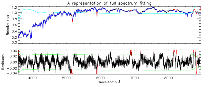
Figure 2.— The combined spectrum of the galaxies in the first redshift bin of the sub-sample II and its best-fit by adopting the GS model. In the top panel, black and blue lines show the combined spectrum and its best-fit model spectrum, respectively. These two spectra are almost superimposed on each other and the black line can be seen only when zooming in the Figure. The cyan line is the multiplicative polynomial to absorb the effects of an imprecise flux calibration and of the Galactic extinction. The red regions are rejected from the fitting (rejection of flagged telluric lines and automatic rejection of outliers). The bottom panel shows the residuals of the best-fit. The solid green lines mark the $1\sigma$ deviation, and the dashed green line represents zero residuals.

Table 3Results of a SSP fitting with the GS model for sub-sample II.

Redshift Interval	SSP-equivalent age	SSP-equivalent [Fe/H]	velocity dispersion
	(Gyr)	(dex)	($\rm km~{}s^{-1}$)
$0.03<z\leq 0.06$	7.13$\pm$0.53	0.17$\pm$0.01	243.5$\pm$4.0
$0.06<z\leq 0.09$	6.52$\pm$0.43	0.17$\pm$0.01	239.2$\pm$3.7
$0.09<z\leq 0.12$	6.31$\pm$0.40	0.16$\pm$0.01	236.0$\pm$3.7
$0.12<z\leq 0.15$	6.01$\pm$0.40	0.17$\pm$0.01	239.0$\pm$3.7
$0.15<z\leq 0.18$	6.11$\pm$0.45	0.15$\pm$0.01	240.7$\pm$3.9
$0.18<z\leq 0.21$	5.49$\pm$0.24	0.18$\pm$0.01	242.4$\pm$3.8
$0.21<z\leq 0.24$	5.37$\pm$0.22	0.17$\pm$0.01	243.0$\pm$3.5
$0.24<z\leq 0.27$	4.98$\pm$0.22	0.15$\pm$0.01	242.7$\pm$3.5
$0.27<z\leq 0.30$	4.96$\pm$0.19	0.14$\pm$0.01	247.6$\pm$3.3
$0.30<z\leq 0.33$	4.78$\pm$0.16	0.12$\pm$0.01	247.4$\pm$3.4
$0.33<z\leq 0.36$	3.82$\pm$0.24	0.16$\pm$0.02	243.7$\pm$3.5
$0.36<z\leq 0.39$	3.64$\pm$0.19	0.17$\pm$0.02	248.9$\pm$3.2

Note. — Column 1 is the redshift interval, columns 2, 3 and 4 are the SSP-equivalent age in unit of Gyr, the [Fe/H] in unit of dex, the velocity dispersion in unit of $\rm km~{}s^{-1}$ and their associated errors, respectively.

Figure 3 illustrates the best fit result obtained by adopting the GS model. The top, middle and bottom panel in the Figure shows the velocity dispersions, metallicities and ages for each redshift bin in each of the four sub-samples, respectively. As seen from the top panel of Figure 3, the fitting results on the velocity dispersions are consistent with the ones given in the MPA/JHU catalogue, which are shown in Figure 3 as open squares, triangles, diamonds, and circles, respectively. The middle panel shows that the galaxies in each sub-sample have similar metallicities, confirming that our samples are almost homogeneous, though of course subtle differences remain. From the bottom panel, it is clear that the mean age ($t_{\rm age}$) decreases with redshifts from $0.03$ to $0.39$. Apparently, the age of the galaxies with higher velocity dispersion tend to be somewhat older than those with lower velocity dispersion, which is consistent with the well known “downsizing” formation of galaxies, i.e., the bigger and more massive galaxies were formed earlier, while the small galaxies formed later (Cowie et al., 1996). Assuming that the $t_{\rm age}-\sigma_{v}$ relation follows a power-law, i.e., $t_{\rm age}\propto\sigma_{v}^{\gamma}$, we fit the relationship for each redshift bin and obtain the slope $\gamma$. The mean value of $\gamma$ for all the redshift bins (and its standard deviation) is $\simeq 0.77\pm 0.25$. We may also first obtain the mean $t_{\rm age}$ for each sub-sample and then fit the mean $t_{\rm age}-\sigma_{v}$ relationship and find $\gamma\simeq 0.79\pm 0.24$.

A number of studies have obtained the relationship between the age ($t_{\rm age}$) and velocity dispersion ($\sigma_{v}$) of early-type galaxies or LRGs and shown that the $t_{\rm age}$ depends $\sigma_{v}$. For example, Caldwell et al. (2003) analyzed the integrated spectra of 175 nearby early-type galaxies by using higher order Balmer lines as the age indicators and found that early-type galaxies with lower $\sigma_{v}$ have smaller luminosity-weighted mean ages. The data obtained by Caldwell et al. (2003) suggests that the slope of the $t_{\rm age}-\sigma_{v}$ relation is roughly $0.8-1.2$ (Nelan et al., 2005). Thomas et al. (2005) studied the spectra of 124 early-type galaxies in both high and low density environments by using the absorption line indices, and they also found that $t_{\rm age}$ correlates with $\sigma_{v}$. Adopting the data in Thomas et al. (2005), the slope of the $t_{age}-\sigma_{v}$ relation is found to be $0.78\pm 0.23$ (Nelan et al., 2005). Nelan et al. (2005) investigated the spectroscopic line strength of 4097 red-sequence galaxies in 93 low-redshift galaxy clusters, and they found $t_{\rm age}\propto\sigma_{v}^{0.59\pm 0.13}$. Smith et al. (2009) studied the spectra of 232 quiescent galaxies in the Shapley supercluster and found $t_{\rm age}\propto\sigma_{v}^{0.40}$. As discussed in Nelan et al. (2005), the differences in sample selection criteria and emission treatment may be account for the differences of $t_{\rm age}-\sigma$ scaling relation. Considering of these differences, our results are well consistent with those obtained by previous works.

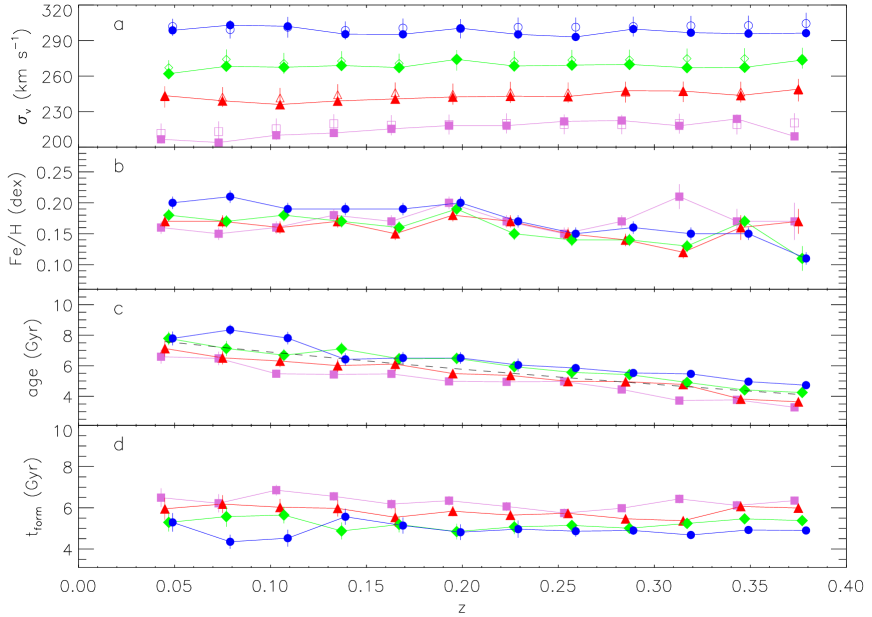
Figure 3.— The mean galactic properties extracted from the combined spectra by using the GS model. Panels (a), (b), (c) and (d) show the velocity dispersions, metallicities, mean luminosity-weighted ages and mean formation time of the LRGs obtained through their combined spectra in each redshift bin for each of the four sub-samples, $200\rm km~{}s^{-1}<\sigma_{v}\leq 230\rm km~{}s^{-1}$ (purple squares), $230\rm km~{}s^{-1}<\sigma_{v}\leq 260\rm km~{}s^{-1}$ (red triangles), $260\rm km~{}s^{-1}<\sigma_{v}\leq 290\rm km~{}s^{-1}$ (green diamonds), and $290\rm km~{}s^{-1}<\sigma_{v}\leq 320\rm km~{}s^{-1}$ (blue circles), respectively. For clarity, those symbols for the same redshift bin but different sub-sample are put offset by $\delta z=-0.002$, $0$, $0.002$, and $0.004$ along the horizontal axis for the four sub-samples with velocity dispersions from low to high, respectively. The galactic velocity dispersions obtained directly from the MPA/JHU catalogue are shown as open squares, triangles, diamonds, and circles for each sub-sample, respectively. In the panel (c), the dashed line indicates $t_{\rm U}(z)-5.5\,\textnormal{Gyr}$, where $t_{\rm U}(z)$ is the age of the universe for a $\Lambda$CDM cosmology and is for reference only. The concordant cosmological model, i.e., $H_{0}=71\rm km~{}s^{-1}~{}Mpc^{-1}$ and $\Omega_{\rm m}=0.27$, is adopted to obtained the mean galaxy formation time shown in panel (d).

3.3.2 Reliability of the fitting results

It is important to check the reliability of the fitting results to ensure it is not highly dependent on the particular synthesis technique adopted, or affected by the existence of multiple solutions due to degeneracies among the model parameters.

Koleva et al. (2008) analyzed the spectra of Galactic clusters using ULySS, and they found that stellar populations of these clusters obtained from the model are well consistent with that obtained from the color-magnitude diagrams. Koleva et al. (2009b) further analyzed the detailed star formation history of 16 dwarf galaxies by using either ULySS or STECKMAP, and they found that the two programs give remarkably consistent results. In addition, Michielsen et al. (2007) adopted two different techniques, i.e., the Lick/IDS index system and the full spectrum fitting method, to test the reliability of the estimates of the ages and metallicities of 16 dwarf elliptical galaxies, and they found these two techniques give consistent results on the age and the metallicity, with an rms error of 1.63 Gyr in age and 0.09 dex in [Z/H]. Du et al. (2010) synthesized the star formation histories and evolution of 35 brightest E+A galaxies from the SDSS DR5, and demonstrated the robustness of the ULySS technique in measuring the age and metallicity of stellar systems. These studies show that the fitting results with different synthesis technique are consistent with each other, and the results of our ULySS fitting should be robust.

We perform Monte-Carlo simulations to visualize the degeneracies and validate the errors by simulating the effect of the noise. For each combined spectrum, we perform 1000 simulations. In each of the simulations a random Gaussian noise is added to the combined spectrum and the amplitude of the added noise is set to the estimated noise associated to the combined spectrum. We then get the mean values of the age, abundance of metallicity and velocity dispersion, and their standard deviations, correspondingly. Figure 4 shows the results of the 1000 Monte-Carlo simulations (open symbols) and the original best fit shown in Figure 3 (filled symbols). According to Figure 4, we conclude that in most of cases, the value of mean velocity desperation and mean age for every bin of the 1000 Monte-Carlo simulations lead to the best fitting solutions, though there are still some deviations especially for sub-sample IV, which may be caused by relatively small number of galaxies used to obtain the combined spectrum. Since we only need to model the age–redshift relation, the diversity of metallicity between the best fitting value and Monte-Carlo simulations value do not affect our conclusion.

The general agreement of the above series tests suggest that the ULySS technique is robust in determining the age, metallicity and velocity dispersion of stellar systems, and the fitting results on the physical properties of galaxies obtained from the full spectrum fitting are also secure.

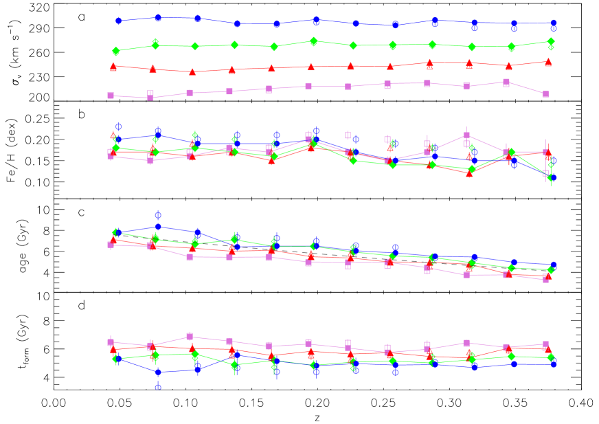
Figure 4.— Legends are similar to that of Figure 3, except that the Monte-Carlo simulation results (open symbols) are additionally shown here. And the Monte-Carlo simulations are performed to visualize the degeneracy and validate the estimation of the errors (see Section 3.3.2).

4. Constraints on the Hubble parameter

The age–redshift relation obtained from observations can be directly fitted by

$$t_{\rm age}=t_{\rm U}-t_{\rm form},$$ (2)

where $t_{\rm age}$ is the mean age obtained from the combined spectrum, $t_{\rm form}$ is the mean formation time of the quiescent galaxies and assumed to be a constant for each sub-sample, and $t_{\rm U}$ is the age of the universe. According to the $\Lambda$CDM cosmology, $t_{\rm U}$ at redshift $z$ is given by

$$t_{\rm U}=\frac{1}{H_{0}}\int_{z}^{\infty}\frac{dz}{(1+z)\sqrt{\Omega_{\rm m}(1+z)^{3}+\Omega_{\Lambda}}},$$ (3)

which depends not only on the value of $H_{0}$ but also the composition of the universe, i.e., $\Omega_{\rm m}$ and $\Omega_{\Lambda}$.

In order to obtain a model-independent measurement of $H_{0}$, however, we first simply assume $H(z)=H_{0}+H^{\prime}z$ (but it may be a good approximation only at low redshift), then the age of the universe is given by

$$t_{\rm U}=\int_{z}^{\infty}\frac{dz}{(1+z)(H_{0}+H^{\prime}z)}.$$ (4)

Using the standard $\chi^{2}$ minimization, we fit the age-redshift relation obtained from each sub-sample to get the best fit of $H_{0}$ and $t_{\rm form}$, and the uncertainty of $H_{0}$ by marginalizing over $H^{\prime}$ and $t_{\rm form}$ (and the uncertainty of $t_{\rm form}$ by marginalizing over $H^{\prime}$ and $H_{0}$). Figure 5 shows the best fit of the age–redshift relation for each sub-sample, respectively. The best fits of the Hubble parameter $H_{0}$ range from $84^{+7}_{-9}\rm km~{}s^{-1}~{}Mpc^{-1}$, $77^{+9}_{-7}\rm km~{}s^{-1}~{}Mpc^{-1}$, $68^{+5}_{-7}\rm km~{}s^{-1}~{}Mpc^{-1}$ to $63^{+7}_{-4}\rm km~{}s^{-1}~{}Mpc^{-1}$ for the sub-samples with velocity dispersions from low to high (see Table 4), but the mean galaxy formation time can not be well constrained. The age–redshift relations obtained from all the four sub-samples can also be fitted simultaneously, and only six parameters are now involved in the fitting, i.e., $H_{0}$, $H^{\prime}$, and the mean formation time of the galaxies in each sub-sample, denoted as $t_{\rm form1}$, $t_{\rm form2}$, $t_{\rm form3}$, and $t_{\rm form4}$, respectively, since $H_{0}$ and $H^{\prime}$ are the same for all the age–redshift relations. By marginalizing over parameters $H^{\prime}$, $t_{\rm form1}$, $t_{\rm form2}$, $t_{\rm form3}$ and $t_{\rm form4}$, we obtain the best-fit of $H_{0}=73^{+4}_{-3}\rm km~{}s^{-1}~{}Mpc^{-1}$ (see the left panels of Figure 6)

Figure 5.— The best fits to the age–redshift relations obtained from each sub-sample (points with errorbars) by assuming $H(z)=H_{0}+H^{\prime}z$ (dashed lines) and a spatially flat $\Lambda$CDM model (solid lines), respectively. The dashed lines almost overlap the solid lines.

Table 4The best fit of the Hubble parameter at the present time $H_{0}$

Sample	$H(z)=H_{0}+H^{\prime}z$			Flat $\Lambda$CDM
	$H_{0}$	$\chi^{2}_{\nu}$		$H_{0}$	$\chi^{2}_{\nu}$
Sub-sample I	$84^{+7}_{-9}$	1.47		$89^{+7}_{-9}$	1.43
Sub-sample II	$77^{+9}_{-7}$	1.26		$83^{+9}_{-8}$	1.21
Sub-sample III	$68^{+5}_{-7}$	0.72		$72^{+6}_{-7}$	0.66
Sub-sample IV	$63^{+7}_{-4}$	0.86		$65^{+7}_{-3}$	0.86
Sub-sample III+IV	$68^{+4}_{-5}$	0.82		$74^{+5}_{-4}$	0.78
All sub-samples	$73^{+4}_{-3}$	1.14		$80^{+2}_{-4}$	1.08

Note. — Here $H_{0}$ is in unit of $\rm km~{}s^{-1}~{}Mpc^{-1}$, $\chi^{2}_{\nu}$ is the reduced $\chi^{2}$. Columns 2 and 3 list the best-fit value of $H_{0}$, its $1\sigma$ error and the reduced $\chi^{2}$, by assuming $H(z)=H_{0}+H^{\prime}z$; while columns 4 and 5 list the best-fit value of $H_{0}$, its $1\sigma$ error and the reduced $\chi^{2}$ by assuming a spatially flat $\Lambda$CDM model.

Assuming spatial flatness for simplicity, we further adopt equation 2 and equation 3 (given by the standard $\Lambda$CDM model) to fit the age–redshift relation obtained from each sub-sample, separately. The best fit of $H_{0}$ is obtained by marginalizing over $\Omega_{\rm m}$ and $t_{\rm form}$ and it ranges from $89^{+7}_{-9}\rm km~{}s^{-1}~{}Mpc^{-1}$, $83^{+7}_{-8}\rm km~{}s^{-1}~{}Mpc^{-1}$, $72^{+6}_{-7}\rm km~{}s^{-1}~{}Mpc^{-1}$ to $65^{+7}_{-2}\rm km~{}s^{-1}~{}Mpc^{-1}$ for the four sub-sample velocity dispersion from low to high, respectively (see Figure 5 and Table 4). We also obtain $H_{0}$ by fitting the age–relations obtained from all the four sub-sample simultaneously by marginalizing over $\Omega_{\rm m}$ and the mean formation time of those galaxies, and the best fit of $H_{0}$ is $80^{+2}_{-4}\rm km~{}s^{-1}~{}Mpc^{-1}$ (see the right panels of Figure 6). And the best fit of $\Omega_{\rm m}$ is $0.09$ and it ranges from $0.08$ to $0.25$, which cannot be constrained with high accuracy. By marginalizing over other parameters, we obtain the best fit of $t_{\rm form1}$, $t_{\rm form2}$, $t_{\rm form3}$, or $t_{\rm form4}$ as $9.7^{+0.3}_{-2.7}$ Gyr, $9.2^{+0.3}_{-2.4}$ Gyr, $8.8^{+0.2}_{-2.3}$ Gyr, or $8.4^{+0.2}_{-2.2}$ Gyr. These values of $t_{form}$ seem to be far too large than the expectation from the standard $\Lambda CDM$ cosmology for LRGs, which are mainly caused by the poorly constrained $\Omega_{m}$ (=0.09). By assuming a flat universe with $\Omega_{m}$=0.27 (the concordant cosmological model) and re-fitting the age-redshift relations for the four velocity dispersion bins simultaneously, the best fit gives $H_{0}=73\rm km~{}s^{-1}~{}Mpc^{-1}$, $t_{form1}=5.9$ Gyr, $t_{form2}=5.4$ Gyr, $t_{form3}=5.0$ Gyr, and $t_{form4}=4.6$ Gyr, respectively. Clearly the mean formation time of those less massive galaxies is smaller than that of those more massive galaxies, which is fully consistent with the “downsizing” evolution nature of galaxy formation. One may also directly obtain the formation time from the age–redshift relations by adopting the concordant cosmological model, i.e., fixing the Hubble constant $H_{0}=71\rm km~{}s^{-1}~{}Mpc^{-1}$, the matter density $\Omega_{\rm m}=0.27$ and dark energy density $\Omega_{\Lambda}=0.73$, the formation time from the age–redshift relations are $t_{\rm form1}=6.2$ Gyr, $t_{\rm form2}=5.7$  Gyr, $t_{\rm form3}=5.3$ Gyr, and $t_{\rm form4}=4.9$ Gyr, respectively. The mean galaxy formation time is about $5.5$ Gyr for the four velocity dispersion bins, which is adopted in Figure 3 (represented by the dashed line). Note that the obtained $t_{\rm form}$ is the average age of a population of galaxies but neither the age of individual galaxies nor the oldest population of stars in those galaxies. Note also there is strong degeneracy between $t_{\rm form}$ and ($H_{0}$,$\Omega_{\rm m}$) obtained from the fitting, which introduces a large uncertainty in the estimation of $t_{\rm form}$.

According to the above fittings, obviously a strong constraint on $H_{0}$ can still be obtained by either assuming a simple model independent form of the evolution of $H(z)$ or a flat universe, i.e., $\Omega_{\rm m}+\Omega_{\Lambda}=1$, although the age–redshift relations are obtained in a limited redshift range and the uncertainties in the age estimates may be substantial. The $H_{0}$ estimated from the sub-sample with lower velocity dispersion tends to be higher than that from the sub-sample with higher velocity dispersion (more massive and luminous LRGs), which may be due to some bias introduced by the systematical difference in the assembly history of less massive galaxies and massive galaxies. Brown et al. (2007) pointed out that the evolution of galaxies in the red sequence is heavily dependent on luminosity, i.e., the lower the luminosity of the galaxies, the more significant the population of new stars formed since $z=1$. So the contamination from the population of stars formed at low redshift (e.g., $z\lesssim 0.4$) is probably more significant in the sub-sample I and sub-sample II than that for the sub-sample III and sub-sample IV. And the age–redshift relation estimated from the lower velocity dispersion sub-sample tends to be shallower than that from the higher velocity dispersion sub-sample, which may lead to an overestimation of the Hubble parameter up to $\sim 20\%$ (see discussions in Section 5.3).

As the possible systematic bias may be not significant for the two subs-samples with high velocity dispersions, we also fit the age–redshift relations obtained from the two sub-samples simultaneously by assuming either a spatially flat $\Lambda$CDM model or $H(z)=H_{0}+H^{\prime}z$. The best fit of $H_{0}$ is either $74^{+5}_{-4}\rm km~{}s^{-1}~{}Mpc^{-1}$ or $68^{+4}_{-5}\rm km~{}s^{-1}~{}Mpc^{-1}$. And the best fit of $\Omega_{\rm m}$ is $0.07^{+0.28}_{-0.01}$ if assuming a spatially flat $\Lambda$CDM model.

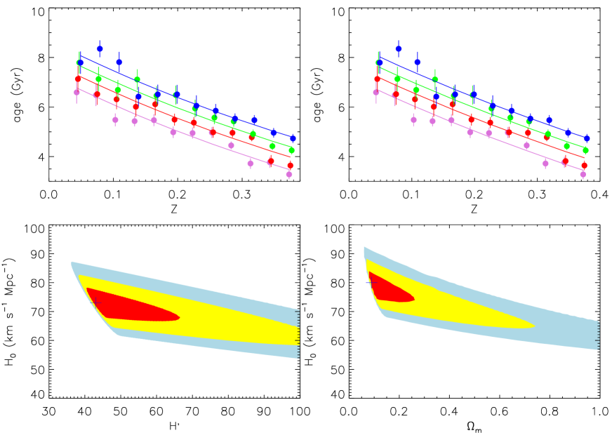
Figure 6.— The best fit to the age–redshift relations by fitting these relations obtained from the four sub-samples simultaneously. Left panels show the results obtained by assuming $H(z)=H_{0}+H^{\prime}z$, while right panels show the results obtained by assuming a spatially flat $\Lambda$CDM model. The top panels show the best fits (lines) to the age–redshift relations (points with errorbars) obtained from the sub-sample I (purple), sub-sample II (red), sub-sample III (green) and sub-sample IV (blue), respectively. The left-bottom panel show the confidence levels of the fitting parameters ($H_{0}$,$H^{\prime}$) by marginalizing over the formation time $t_{\rm form1}$, $t_{\rm form2}$, $t_{\rm form3}$, $t_{\rm form4}$, and the right bottom panel shows the confidence levels of the fitting parameters ($H_{0}$,$\Omega_{\rm m}$) by marginalizing over $t_{\rm form1}$, $t_{\rm form2}$, $t_{\rm form3}$, $t_{\rm form4}$. The crosses denote the positions of the best fits, the contours correspond to the $1\sigma$, $2\sigma$, $3\sigma$ levels, respectively.

Considerable progress has been made in determining the Hubble parameter over the past two decades by using many different techniques (e.g., Freedman & Madore, 2010). For example, the Hubble parameter is estimated to be $H_{0}=73\pm 5\rm km~{}s^{-1}~{}Mpc^{-1}$ by using the tip of the red giant branch as an alternate calibration to the Cepheid distance scale (Mould & Sakai, 2008); $72\pm 4(random)\pm 11(systematic)\rm km~{}s^{-1}~{}Mpc^{-1}$ by using the surface brightness fluctuation to determine cosmic distances (Blakeslee et al., 2002); $74.3\pm 3.6\rm km~{}s^{-1}~{}Mpc^{-1}$ by using Type Ia supernovae (Riess et al., 2009); $76.9^{+3.9+10}_{-3.4-8.0}\rm km~{}s^{-1}~{}Mpc^{-1}$ by using the Sunyaev-Zel’dovich effect (Bonamente et al., 2006); and $68\pm 2\rm km~{}s^{-1}~{}Mpc^{-1}$ by using the BAO signature in the matter power spectrum (Percival et al., 2010). The Hubble Space Telescope key project yielded a consistent value of $H_{0}=72\pm 3(random)\pm 7(systematic)\rm km~{}s^{-1}~{}Mpc^{-1}$ by combining the data obtained from different techniques (Freedman & Madore, 2010). Komatsu et al. (2009) also obtained a value of $H_{0}=70.5\pm 1.3\rm km~{}s^{-1}~{}Mpc^{-1}$ by combining the WMAP-5 data with the SNe Ia and BAO data, while Tammann et al. (2008) found consistently low values of $H_{0}$, from several different tracers they obtain a mean value of $H_{0}=62.3\pm 1.3\rm km~{}s^{-1}~{}Mpc^{-1}$. Considering of the possible systematic error in the $H_{0}$ estimation by using the age–redshift relation, our estimates of $H_{0}$ are fully consistent with those listed above.

5. Discussion

In this paper, we have obtained the mean age, metallicity and velocity dispersion for a sample of quiescent galaxies selected from the SDSS DR7 in different redshift bins. The age-redshift relation derived from those quiescent galaxies is consistent with the expectation from the $\Lambda$CDM cosmology and may provide a good estimate of the Hubble parameter ($H_{0}$). However, the estimate of $H_{0}$ is valid only if those quiescent galaxies are passively evolving and the galaxies in different redshift bins represent the same population formed more or less at the same time. In order to check whether these requirements are satisfied for the quiescent galaxy sample selected in this paper, we perform some tests below to investigate the evolution effects due to different star formation history or galaxy mergers, and illustrate that those quiescent galaxies are indeed more or less formed at the same epoch using the evolution of their average colors.

5.1. Star formation history

According to the selection criteria, most galaxies in our sample should be quiescent galaxies and supposed to be passively evolving. However, the star formation history of those galaxies may not be a single burst. To test whether there are significant younger stellar populations in the galaxies, we re-do the full spectrum fitting for each combined spectrum by adopting two stellar components, one young stellar population (YSP) and one old stellar population (OSP). The age of the young stellar population is assumed to be in the range from $0.1$ Gyr to $1$ Gyr, while for the old population it is assumed to be in the range from $1$ Gyr to $15$ Gyr. For both populations, the metallicity is a free parameter without restrictions. According to the fitting results, we note here that the fitting age of the YSP always reaches the edge of its limits (the age of YSP is always either $0.1$ Gyr or $1$ Gyr), which means that a YSP with an age in the given range can not be found. Furthermore, even if there exist a YSP, the light fraction (LF) is very small ($2.8\%$ on average) so that it can be neglected. Therefore, we conclude that the YSP (the age of which $\textless 1$ Gyr) is negligible and not required in the fitting. We also test the cases by setting a larger upper limit on the age of the YSP, e.g., $2$ Gyr, $3$ Gyr or even $4$ Gyr (or alternatively a lower limit on the age of the old stellar population, i.e., $4$ Gyr to $6$ Gyr), and also find that no significant YSP is required by the fitting. All these tests suggest that most of the quiescent LRGs may be passively evolving and not experience significant recent ($\lesssim 2$ Gyr) star formation. For those galaxies at low redshift bins, however, we find there may exist YSP’s with age $\sim 3$ Gyr, possibly due to the later major mergers (see discussions in Section  5.3).

To close this sub-section, we note here that Tojeiro & Percival (2010) find bright LRGs being consistent with pure passive evolution while faint LRGs slightly deviating from pure passive evolution as revealed by the evolution of the number and luminosity density of LRGs as well as that of their clustering. The lesser passiveness of LRGs with smaller velocity dispersion seems not to be able to be directly revealed by the combined spectra of LRGs studied in this paper, which might be due to that the signature of YSPs (probably with quite different ages) in (some of) the LRGs may be diluted or smoothed due to the co-adding of a large number of LRG spectra in our analysis. High S/N spectra of individual LRGs may be helpful to clarify the less passiveness of small LRGs, however, the S/N of most LRGs in our sample are only slightly larger than 10 and not sufficiently high for clarifying this problem.

5.2. Combined spectrum vs. single spectrum

The combined spectrum in each redshift and velocity bin may only represent the mean spectrum of galaxies in that bin. Does the physical properties derived from the model fitting of this combined spectrum represent the mean properties of all galaxies in that bin? In order to test this, we fit each single spectrum for all the galaxies in each velocity dispersion bin and redshift bin with ULySS. The initial settings are the same as that in Section 3.3.1. After obtaining the best fit of the age for each single spectrum, we calculate the mean of the ages of those galaxies which belong to the same velocity dispersion and redshift bin and its standard deviation. Figure 7 shows the mean age-redshift relation for every single spectrum. As seen from Figure 7, the mean age-redshift relation obtained from the single spectrum fitting is still consistent with that obtained from the combined spectra but with much larger errors.

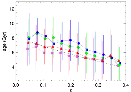
Figure 7.— The mean age-redshift relation derived by fitting each single spectrum in the LRG sample with ULySS for each redshift bin of each of the four sub-samples, $200\rm km~{}s^{-1}<\sigma_{v}\leq 230\rm km~{}s^{-1}$ (purple squares), $230\rm km~{}s^{-1}<\sigma_{v}\leq 260\rm km~{}s^{-1}$ (red triangles), $260\rm km~{}s^{-1}<\sigma_{v}\leq 290\rm km~{}s^{-1}$ (green diamonds), and $290\rm km~{}s^{-1}<\sigma_{v}\leq 320\rm km~{}s^{-1}$ (blue circles), respectively. The dashed line indicates $t_{\rm U}(z)-5.5\,\textnormal{Gyr}$ , where $t_{\rm U}(z)$ is the age of the universe for a $\Lambda$CDM cosmology and is for reference only.

5.3. Major mergers of quiescent galaxies

The differences among the model spectra become small if the ages of the stellar populations are larger than $4$ Gyr. Therefore, the uncertainties in the estimates of the ages and metallicities of galaxies with low $S/N$ spectra are substantial. For this reason, we have combined the spectra of galaxies in each redshift and velocity dispersion bin together to improve the $S/N$. However, the age difference obtained by modeling the combined spectra can represent the age difference of the universe only if those galaxies at different redshifts are the same population and were formed more or less in the same epoch. There is a potential caveat to this approach, i.e., if a significant fraction of quiescent galaxies experience major mergers and thus some star formation at low redshift $z\lesssim 0.4$, then some quiescent galaxies in the redshift bin $0.03-0.06$ were formed at $z<0.4$ and they were not represented by those galaxies in the redshift bin $0.36-0.39$. It is important to check the effect of the major merger of galaxies on the age-redshift relation.

The major merger rate of galaxies is defined as the number of mergers per galaxy with mass larger than a threshold ($M_{\ast}$) per unit time and denoted as $dN_{\rm mrg}/dt$, and it can be roughly estimated by the fitting formula given by Hopkins et al. (2010), i.e.,

$$\frac{{\rm d}N_{\rm mrg}}{{\rm d}t}=A(M_{\rm min})(1+z)^{\beta(M_{\rm min})}[{\rm per\ galaxy}],$$ (5)

where the normalization is

$$A(M_{\rm min})_{\rm major}\approx 0.02[1+(M_{\rm min}/M_{0})^{0.5}]{\rm Gyr^{-1}},$$

and the redshift evolution is

$$\beta(M_{\rm min})_{\rm major}\approx 1.65-0.15\log(M_{\rm min}/M_{0}),$$

and $M_{0}\equiv 2\times 10^{10}\,{M_{\sun}}$. For the galaxies in our sample, they are generally brighter than $3L^{\ast}$ (Eisenstein et al., 2001) and have stellar masses in the range from $10^{11}{M_{\sun}}$ to a few times $10^{12}{M_{\sun}}$ according to Tal et al. (2011). Assuming that the minimum mass of those galaxies is $M_{\rm min}=10^{11}{M_{\sun}}$, the average number of major mergers experienced by a galaxy at redshift $z$ since $z=0.40$ is

$$N_{\rm mrg}(z)=\int_{z}^{0.40}\frac{dN_{\rm mrg}}{dt}|\frac{dt}{dz}|dz,$$ (6)

where $dt/dz$ is given by Eq. (1). The fraction of galaxies in a redshift bin $z\pm dz$ which experienced major mergers since $z=0.4$ is $\sim N_{\rm mrg}(z)$, and $N_{\rm mrg}(z)\sim 0.33$, $0.26$, and $0.01$ at $z=0.03$, $0.11$, and $0.39$ for our sample, respectively. Note that almost all the major mergers are dry mergers for massive galaxies with mass $>10^{11}M_{\odot}$ similar to that in our sample (Hopkins et al., 2010). These dry mergers may also lead to new star formation or star burst in the galactic centers, and thus introduce a systematic bias to the age–redshift relation, because the mean age obtained from the combined spectra by the GS model at low redshift bins may be systematically underestimated due to the additional population of stars formed later.

We check the effect of these major mergers on the age–redshift relation as following. First, we assume an underlying age-redshift relation according to the $\Lambda$CDM, i.e., the age of the galaxy at redshift $z$ is $t_{\rm U}(z)-t_{\rm form}$, and $H_{0}=71\rm km~{}s^{-1}~{}Mpc^{-1}$, $\Omega_{\rm m}=0.27$, $t_{\rm form}=5.5~{}{\rm Gyr}$ are assumed. Here $t_{\rm form}=5.5~{}{\rm Gyr}$ is adopted according to the average formation time obtained by fitting the age-redshift relation for four velocity dispersion bins (see Section  4 for details). However, Thomas et al. (2005) found that vigorous star formation episodes in massive galaxies ofter occur at $z\sim 2-5$, corresponding to a cosmic age of less than $3.3$ Gyr. The $t_{form}$ obtained from the age–redshift relations for the quiescent LRGs in this paper is larger than that obtained by Thomas et al. (2005), which needs further investigation. As the galaxies in our sample are all LRGs, the age of the newly formed stellar population by major mergers, if significant, is at least $1$ Gyr, which corresponds to $\delta_{\rm z}\sim 0.1$, as the migration of galaxies driven by mergers from blue cloud to red sequence may last $\sim 1$ Gyr (see Schawinski et al., 2010). If a galaxy at redshift $z$ is the remnant of a major merger, the age of the younger stellar population in it is approximately $1/2[t_{\rm U}(z)-t_{\rm U}(z=0.4)]+1{\rm Gyr}$. Then a “forged” combined spectrum of galaxies at redshift bin z can be approximately generated by two stellar populations, i.e., an old stellar population with the age $t_{\rm U}(z)-t_{\rm form}$, and a young stellar population with age $\sim 1/2[t_{\rm U}(z)-t_{\rm U}(z=0.4)]+1{\rm Gyr}$. The fraction of major mergers is

$$N_{\rm mrg}({z+\delta_{\rm z}})=\int_{z+{\delta_{\rm z}}}^{0.40+\delta_{\rm z}}\frac{dN_{\rm mrg}}{dt}\left|\frac{dt}{dz}\right|dz.$$

Hopkins et al. (2010) have shown that the fraction of the young population generated by major mergers is $\sim 0.05-0.10$ in galaxies with $>10^{11}M_{\odot}$ (see their Figure 14). Here we assume it is $\sim 0.07$. Note that this fraction may be an upper limit as the LRGs studied here are quiescent ones, in which the star formation generated by major mergers might be even less. Therefore, the fraction of the young population contributing to the combined spectrum is $\sim 0.07\times N_{\rm mrg}(z)$, and the fraction of the old population is $1-0.07\times N_{\rm mrg}(z)$. We fit these spectra obtained for each redshift by the same method as that in Section 3.3.1 and obtain the age for these combined spectra. Similar to that in Section 4, we obtain the best fit of $H_{0}=86^{+2}_{-4}\rm km~{}s^{-1}~{}Mpc^{-1}$ by fixing $\Omega_{\rm m}=0.27$.

From the above calculation, we conclude that $H_{0}$ may be systematically overestimated by up to $\sim 20\%$ if using the age-redshift relation obtained from the combined spectra. Considering this systematic bias, $H_{0}$ estimated from the age–redshift relation in this paper is consistent with those estimated by other techniques. Note also that the systematic bias introduced to the $H_{0}$ estimate appears not significant for the two sub-samples with the highest velocity dispersions, which might mean that those very massive LRGs are really quiescent and have approximately zero star formation at redshift $z\lesssim 0.4$. Tojeiro & Percival (2010) have pointed out that the brightest galaxies show the smallest departure from pure passive evolution. Therefore, the most massive LRGs with velocity dispersion $\gtrsim 300\rm km~{}s^{-1}$ may be efficient tools to constrain the cosmological parameters, such as $H_{0}$, through the age–redshift relations extracted from their spectra.

We also check whether the g-r color of the galaxies having the combined spectra in each redshift bin is consistent with that of the model galaxies that have the same spectrum as the combined spectrum in the highest redshift bin. To do this, we extract a model spectrum from the GS model grid, whose age and metallicity are the best fitting results with ULySS for redshift bin 0.36-0.39, then we let this spectrum evolve toward the low redshift. That is, if the age and metallicity of the combined spectrum are t and $Z_{\rm Fe/H}$ at z=0.375, then at a low redshift z, we extract a spectrum from model grid whose age is $t+\delta t$ and let the metallicity is fixed to $Z_{\rm Fe/H}$, where $\delta t=t_{\rm U}(z)-t_{\rm U}(z=0.375)$. We repeat this process till z=0.045, and denote the spectra obtained from the above processes as the “forged spectra”. For each combined spectrum there is also a model spectrum to fit it. We denote this spectrum as the “model spectrum”. Then we calculate the g-r color with SDSS filter of those “forged spectra” and “model spectra” with IRAF task SYNPHOT. We find that the g-r color of the “model spectra” are almost the same as that of the “forged spectra”, which means that the merger effect is not significant for our sample. Furthermore, we pick out those spectrum whose $S/N>30$ from our sample as a sub-sample to derive their physical property with full spectrum fitting. This sub-sample has 1386 galaxies, and these are almost all concentrated in the redshift range from 0.02 to 0.2. We fit these galaxies with SSPs. The initial settings are the same as that in Section 3.3.1. Similarly, we extract the corresponding spectrum from the GS model according to the best fit. Then we calculate the g-r color and find that dispersion of the g-r color is very small compared with that of the combined spectrum, which means the results of the single spectrum are consistent with that of the combined spectrum.

5.4. Model dependence

In this paper, we use the GalexEV/SteLib model to fit the combined spectra, as its wavelength coverage is wider compared with the other models provided by the ULySS package. For completeness, we also test the Pegase-HR/Elodie3.1 model and the Vazdekis/Miles model, and find there is some model dependence. The model dependence may be caused by the limitation of wavelength coverage as the Pegase-HR/Elodie3.1 model covers the wavelength from $3900$Å$-6800$Å, and for the Vazdekis/Miles model it is $3540$Å$-7409$Å. This result is consistent with that of Verkhodanov et al. (2005), in which they analyzed the photometric data of a large sample of elliptical galaxies and found that $H_{0}=72\pm~{}10\rm km~{}s^{-1}~{}Mpc^{-1}$ and $53\pm 10~{}\rm km~{}s^{-1}~{}Mpc^{-1}$ for two different stellar population synthesis models, i.e., PEGASE and GISSEL , respectively. The main ingredients of those models are the stellar evolution tracks, the stellar library, the IMF, the grids of ages and metallicities, and the SFHs, etc. Each model may have different settings in one or more of those ingredients. As demonstrated by Chen et al. (2010), at present there are still some differences in the output between these different models. The model dependence may be avoidable if carefully choosing a compatible stellar population synthesis model for the problem to be studied. We note here that is also interesting to test the model given by Maraston & Stromback (2011), which is based on the fuel consumption theorem and quite different from the other models. However, it is not easy to test this model because it is not yet included in the ULySS code.

From the above tests, we conclude that the age–redshift relation obtained from the combined spectra of a large sample of quiescent LRGs can be used to constrain the Hubble parameter $H_{0}$ (and possibly other cosmological parameters if combining with other data sets). If a large sample of very massive quiescent LRGs can be obtained by the future surveys, such as the Baryon Oscillation Spectroscopic Survey (BOSS), which is less affected by the systematic bias due to new star formation at low redshift, the $H_{0}$ may be able to be determined with substantial accuracy.

6. Conclusions

In this paper, we selected $23,883$ quiescent LRGs from the SDSS DR7 in the redshift range from $0.03$ to $0.39$, by setting a threshold of zero emission (at a $2-\sigma$-level) of the H_α and [Oii] lines directly obtained from the MPA/JHU catalogue. The quiescent LRG sample is divided into four sub-samples according to galaxy velocity dispersions. For each sub-sample, the spectra of galaxies in each of the $12$ redshift bins (from $z=0.03$ to $0.39$ with a step of $\delta z=0.03$) are combined together to obtain a high $S/N$ combined spectrum. Using the full spectrum fitting method, the luminosity-weighted physical properties, such as the velocity dispersion, the metallicity and the age, of those quiescent LRGs are obtained from the combined spectra by adopting a single population synthesis model, i.e., the GalexEV/SteLib model. Using Monte-Carlo simulations, we find that the model results are robust and reliable. We argue that the age–redshift relation estimated from the LRG sample could be systematic biased because of the contamination from a possible younger stellar population formed at $z\lesssim 0.4$ as consequence of major mergers. This bias is most significant for LRGs with smaller velocity dispersions but insignificant for the most massive LRGs. Considering of this systematic bias, the age–redshift relation obtained from the model fittings is fully consistent with the expectations from the $\Lambda$CDM cosmology.

The Hubble parameter $H_{0}$ is first estimated by using the age–redshift relation obtained from each sub-sample, and its value ranges from $89^{+7}_{-9}\rm km~{}s^{-1}~{}Mpc^{-1}$, $83^{+9}_{-8}\rm km~{}s^{-1}~{}Mpc^{-1}$, $72^{+6}_{-7}\rm km~{}s^{-1}~{}Mpc^{-1}$, to $65^{+7}_{-3}\rm km~{}s^{-1}~{}Mpc^{-1}$ for the four sub-samples with velocity dispersions from low to high, respectively. The large value of the $H_{0}$ estimated from the sub-samples with low velocity dispersion is probably due to the systematic bias, which can be as high as $\sim 20\%$. Using the age–redshift relations obtained from the two sub-samples with high velocity dispersions or the sub-sample with the largest velocity dispersion, we find $H_{0}=74^{+5}_{-4}\rm km~{}s^{-1}~{}Mpc^{-1}$ or $H_{0}=65^{+7}_{-3}\rm km~{}s^{-1}~{}Mpc^{-1}$ if assuming a spatially flat $\Lambda$CDM cosmology, which may be less affected by the systematic bias, close to the true $H_{0}$, and are well consistent with the best estimates through other techniques. However, it needs further test on whether those most massive galaxies are truly passively evolving or not.

In summary, we have demonstrated that the age–redshift relation of quiescent galaxies can be reliably estimated by using the full spectral fitting method if the $S/N$ of their spectra are sufficiently high. We conclude that some cosmological parameters, such as the Hubble parameter, can be constrained with considerable accuracy through the age–redshift relation obtained from those most massive LRGs, which is totally independent of other methods. With future surveys like BOSS, the Hubble parameter may be tightly constrained by the age–redshift relation obtained from the most massive quiescent LRGs.

References

- Abazajian et al. (2009) Abazajian, K., et al., 2009, ApJS, 182, 543
- Bertelli et al. (1994) Bertelli, G., Bressan, A., Chiosi C., Fagotto, F. & Nasi, E., 1994, A&A, 106, 275
- Blakeslee et al. (2002) Blakeslee, J. P., et al. 2002, MNRAS, 330, 443
- Bonamente et al. (2006) Bonamente, M., et al., 2006, ApJ, 647, 25
- Bruzual & Charlot (2003) Bruzual, G., Charlot, S. 2003, MNRAS, 344, 1000B
- Brown et al. (2007) Brown M. J. I., Dey A., Jannuzi B. T., Brand K., Benson A. J., Brodwin M., Croton D. J., Eisenhardt P. R., 2007, ApJ, 654, 858
- Caldwell et al. (2003) Caldwell, N., Rose, J. A., Concannon, K. D., 2003, AJ, 125, 2891
- Carson & Nichol (2010) Carson, D. P. & Nichol, R. C. 2010, MNRAS, 408, 213
- Chabrier & Gilles (2003) Chabrier, Gilles, 2003, PASP, 115, 763
- Chen et al. (2010) Chen, X. Y., Liang, Y. C., Hammer, F., Prugniel, Ph., Zhong, G. H., Rodrigues, M., Zhao, Y. H., Flores, H. 2010, A&A, 515, 101
- Cimatti et al. (2008) Cimatti, A., Cassata, P., Pozzetti, L. et al. 2008, A&A, 482, 21
- Cowie et al. (1996) Cowie, L. L., Songaila, A., Hu, E. M., & Cohen, J. G. 1996, AJ, 112, 839
- Cowie et al. (1999) Cowie, L. L., Songaila, A. & Barger, A.J. 1999, AJ, 118, 603
- Crawford et al. (2010) Crawford, S. M., Ratsimbazafy, A. L., Cress C. M., Olivier, E. A., Blyth, S. L. & van der Heyden K.J., MNRAS, 406, 2569
- Diaz et al. (1989) Diaz, A. I., Terlevich, E., & Terlevich, R. 1989, MNRAS, 239, 325
- Du et al. (2010) Du W,Luo A.L., Prugniel Ph., Liang Y.C. & Zhao Y.H. 2010,MNRAS, 409, 567
- Dunlop et al. (1996) Dunlop, J., Peacock, J., Spinrad, H., Dey, A., Jimenez, R., Stern,D., & Windhorst, R., 1996, Nature, 381,581
- Eisenstein et al. (2001) Eisenstein, D. J., et al., 2001, AJ, 122, 2267
- Freedman & Madore (2010) Freedman, W. L., Madore, B. F. 2010, ARA&A, 48, 673
- Heavens et al. (2004) Heavens, A., Panter, B., Jimenez, R. Dunlop, J. 2004, Nature, 428, 625
- Hogg et al. (2001) Hogg, D. W., Finkbeiner, D. P., Schlegel, D. J., Gunn, J. E., 2001, AJ, 122, 2129H
- Hopkins et al. (2010) Hopkins, P. F., et al. 2010, ApJ, 715, 202
- Jimenez & Loeb (2002) Jimenez, R. & Loeb, A. 2002, ApJ, 573, 37
- Jimenez et al. (2003) Jimenez, R., Verde, L., Treu, T. et al. 2003, ApJ, 593, 622
- Jimenez et al. (2004) Jimenez, R., MacDonald, J., Dunlop, J. S., Padoan, P., & Peacock, J. A., 2004, MNRAS, 349, 240
- Koleva et al. (2008) Koleva, M., Prugniel, Ph., Ocvirk, P., Le Borgne, D.& Soubiran, C., 2008, MNRAS, 385, 1998
- Koleva et al. (2009a) Koleva, M., Prugniel, Ph., Bouchard, A.& Wu, Y., 2009a , A&A, 501, 1269
- Koleva et al. (2009b) Koleva, M., Rijcke, S. D., Prugniel, Ph., Zeilinger, W. W. & Michielsen, D.,2009b, MNRAS, 396, 2133
- Komatsu et al. (2009) Komatsu, E. et al., 2009, ApJS, 180, 330
- Maraston & Stromback (2011) Maraston, C. & Stromback, G. 2005, MNRAS, 418, 2785
- Michielsen et al. (2007) Michielsen, D., Koleva, M., Prugniel, Ph., Zeilinger, W. W., Rijcke, S. D., Dejonghe, H., Pasquali, A., Ferreras, I., Debattista, & V. P., 2007, ApJ, 670, L101
- Mould & Sakai (2008) Mould J., Sakai S. 2008, ApJ, 686, L75
- Nelan et al. (2005) Nelan, J. E., Smith, R. J., Hudson, M.J., Wegner, G. A., Lucey, J. R., Moore, S. A. W., Quinney, S. J., Suntzeff, N. B., 2005, ApJ, 632, 137
- Percival et al. (2010) Percival, W. J., et al., 2010, MNRAS, 401, 2148
- Pier et al. (2003) Pier, J. R., Munn, J. A., Hindsley, R. B., Hennessy, G. S., Kent, S. M., Lupton, R. H., & Ivezić, Željko, 2003, AJ, 125, 1559P
- Riess et al. (2009) Riess A. G., et al., 2009,ApJ, 699, 539
- Schawinski et al. (2010) Schawinski, K., Dowlin, N., Thomas, D., Urry, C. M., Edmondson, E. 2010, ApJ, 714, 108
- Schlegel et al. (1998) Schlegel, D. J., Finkbeiner, D. P. & Davis, M. 1998, ApJ, 500, 525
- Simon et al. (2005) Simon, J., Verde, L., & Jimenez, R., 2005, Phys. Rev. D, 71, 123001
- Smith et al. (2009) Smith, R. J., Lucey, J. R., & Hudson, M. J., 2009, MNRAS, 400, 1690
- Spinrad et al. (1997) Spinrad, H., Dey, A., Stern, D., Dunlop, J., Peacock, J., Jimenez,R., & Windhorst, 1997,ApJ,484, 581
- Tal et al. (2011) Tal, T., et al. 2011, arXiv: 1108.1392
- Tammann et al. (2008) Tammann, G. A., Sandage, A., & Reindl, B., 2008, ARA&A, 15, 289
- Thomas et al. (2005) Thomas, D., Maraston, C., Bender, R., & Mendes de Oliveira, C. 2005,ApJ, 621, 673
- Thomas et al. (2010) Thomas, D., Maraston, C., Schawinski, K. et al. 2010, MNRAS, 404, 1775
- Tojeiro & Percival (2010) Tojeiro, R., & Percival, W. J., 2010, MNRAS, 405, 2534
- York et al. (2000) York, D.G., et al., 2000, AJ, 120, 1579
- Verkhodanov et al. (2005) Verkhodanov, O. V., Parijskij, Y. N.,& Starobinsky, A. A., 2005, Bull. Special Astrophys. Obs., 58, 5