Periodic frequencies of the cycles in $2\times 2$ games: evidence from experimental economics

Abstract

Evolutionary dynamics provides an iconic relationship—the periodic frequency of a game is determined by the payoff matrix of the game. This paper reports the first experimental evidence to demonstrate this relationship. Evidence comes from two populations randomly-matched $2\times 2$ games with 12 different payoff matrix parameters. The directions, frequencies and changes in the radius of the cycles are measured definitively. The main finding is that the observed periodic frequencies of the persistent cycles are significantly different in games with different parameters. Two replicator dynamics, standard and adjusted, are employed as predictors for the periodic frequency. Interestingly, both of the models could infer the difference of the observed frequencies well. The experimental frequencies linearly, positively and significantly relate to the theoretical frequencies, but the adjusted model performs slightly better.

1 Introduction

Game theory, including classical game theory VonNeumann1944 and evolutionary game theory Maynard1982evolution , provides a mathematical framework for systems ranging from microbial Frey2010 to social economy myerson1997game . However, the theoretical predictions of classical game theory and evolutionary game theory sometimes differ, two typical examples of this being the Matching Pennies game Dawkins1976 ; Sigmund1981 ; cremer2008anomalous ; claussen2007drift and the Rock-Paper-Scissors game. In these games, evolutionary game theory predicts clear cyclic motions in social state space Taylor1978 ; Sigmund1981 ; Weibull1997 ; Hofbauer2003 ; Sandholm2011 , while classical game theory does not.

As a major source of knowledge in social sciences Falk2009 , laboratory experiments have been employed to test evolutionary game theory Samuelson2002 . Although experiments have supported the existence of the cycles Samuelson2002 ; Binmore2001 ; Friedman1996 ; Plott2004globalScarf , the definitive measurement of cycles has rarely been reported. Quite recently, in a continuous time and centralised information protocol, cycles have been found in Rock-Paper-Scissors (RPS)-like games Friedman2012 . In addition, Xu, Zhou and Wang have studied cycles in standard RPS games with a random matching and decentralised information protocol Xu20134997 . They proved that cycles do exist in continuous time RPS-like games Friedman2012 and discrete time standard RPS games Xu20134997 . Additionally, the directions of all of the cycles detected in these RPS experiments met the evolutionary dynamics very well Friedman2012 ; Xu20134997 . Therefore, we can say that the cycles in the experiments are qualitatively consistent with the expectations of evolutionary game theory.

Subsequently, a straightforward question arises, namely what is the quantitative relationship between cycles in experiments and the parameters of the games? To answer this question, we look to the central frequencies of the cycles which can be (1) measured definitively in experiments and (2) explicitly calculated based on dynamics equations.

Our data is from Selten and Chmura’s experiments of twelve $2\times 2$ games selten2008 (see Fig. 1 and Table 1). According to replicator dynamics models Taylor1978 ; Maynard1982evolution ; Weibull1997 ; Traulsen2005 , the payoff matrices of the twelve games indicate that the transits among social states in each game should form endless cycles. As mentioned in Ref. Nowak2012 , evolutionary game theory has rarely been supported by human experiments. In this article, we will reveal the cycles in the 12 experiments.

With methods rooted in non-equilibrium statistical physics Xu20134997 , we counted the cycles chronologically in the experiments. The main results include: (1) cycles exist; (2) cycles are persistent; (3) the empirical cyclic frequencies in the 12 games are quantitatively different, see Table 2. Moreover, the differences could be well described by the theoretical frequencies derived from replicator dynamics models, see Table 3.

The structure of this paper is as follows. In the next section, we will briefly introduce the 12 experiments and provide the theoretical predictions for the cycles. In Section 3, the measuring methods for the cycles are explained. Section 4 summarises the results. The last section includes discussions and summary.

2 Experiments and Theoretical expectations

To capture the cyclic social behaviours in laboratory game experiments, we use the existing well-known experimental data of Selten and Chmura selten2008 and refer to two theoretical models of evolutionary dynamics Taylor1978 ; Maynard1982evolution ; Weibull1997 ; Traulsen2005 , standard replicator dynamics and adjusted replicator dynamics.

2.1 Two-population $2\times 2$ games experiments

The original aim of Setlen and Chumra’s experimental investigation is to compare the performance of the five stationary concepts selten2008 . They designed twelve $2\times 2$ cyclic matching-pennies-like games Traulsen2005 ; cremer2008anomalous . Games 1 to 6 are constant-sum games, and each of them contains 12 groups; games 7 to 12 are non-constant-sum games, and each of them contains 6 groups. In addition, games 7 to 12 have the same Nash equilibria as the games 1 to 6, respectively.

Each of the 108 groups consists of two four-person populations, so a total of 864 subjects are involved in the experiments. Each group plays the game for 200 rounds repeatedly. The strategy set for each player in the first population (denoted by $X$) is ($X_{1}$,$X_{2}$); while the strategy set for each player in the second population (denoted by $Y$) is ($Y_{1}$,$Y_{2}$). In each round, every subject plays the game against an opponent randomly picked from the other population. The payoff matrix for each game has the same form as Fig. 1 shows, where $a_{ij}$ ($b_{ij}$) indicates the payoff for the player in the first (second) population, $i,j=1,2$. The specific value of $a_{ij}$ ($b_{ij}$) in each game is exhibited in Table 1.

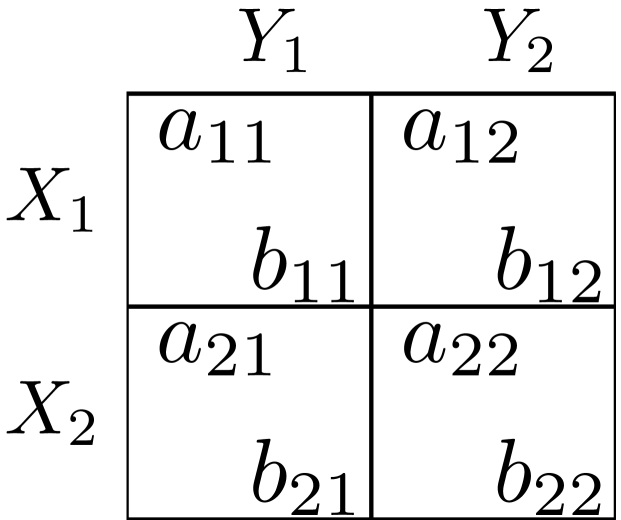
Figure 1: Payoff matrix of the $2\times 2$ game. For the 12 games, the elements of the payoff matrix are different, see Table 1.

2.2 Predictions from two replicator dynamics

As an approximation, evolutionary game dynamics can be a powerful tool to describe finite population games Borgers1997 ; Friedman1998 ; Samuelson2002 ; Friedman2012 . It takes the social state, i.e. the combination of the densities of strategies in each population Sandholm2011 , as a crucial object and analyses its motion in state space. In this case, each social state is denoted as $x$:=$(p,q)$, where $p$ ($q$) is the density of $X_{1}$ ($Y_{1}$) in the first (second) population $X(Y)$ and the state space is $\mathbb{X}$=$\{0,\frac{1}{4},\frac{2}{4},\frac{3}{4},1\}\times\{0,\frac{1}{4},\frac{2}{4},\frac{3}{4},1\}$, as in Fig. 2 (for more details, see Appendix A). According to evolutionary game dynamics, the social state will change in the state space.

As predictors, the two models—standard replicator dynamics and adjusted replicator dynamics—are used as references. The advantage of the two models is that they are parameter free and the most widely used Traulsen2005 ; Maynard1982evolution ; Sandholm2011 ; Friedman1996 ; cremer2008anomalous . The solutions in a (sufficiently small) neighbourhood of the Nash equilibrium can be calculated for the two dynamics for the twelve games. According to the calculation, the motions in these games are cyclic (see Appendix A) and equivalent to two-dimensional simple harmonic motions (see Appendix J in Maynard1982evolution ). Therefore, based on these two models, the observed social state is supposed to keep moving in the state space Taylor1978 ; Maynard1982evolution ; Weibull1997 ; Traulsen2005 and thus form endless cycles, which leads to the following theoretical predictions:

1. The cycles, for all 12 games, exist and persist. Meanwhile, the directions of the cycles are all clockwise.

2. The frequencies of the cycles are different (for numerical results see Table 1, in which $f_{s}$ and $f_{a}$ respectively indicate the predictions from standard and adjusted replicator dynamics).

3. The radius of the cycles, for all 12 games, should remain unchanged over time.

With 12 experimental $2\times 2$ games, we verify the existence and persistence of the cycles; and test the frequencies of cycles quantitatively. Furthermore, we find that the observed periodic frequencies of the cycles are different among games. Moreover, the experimental frequencies are linearly, positively and significantly related to the theoretical frequencies.

Table 1: Payoff matrices, equilibrium, eigenvalues and theoretical frequencies.

Game	$a_{11}$	$b_{11}$	$a_{12}$	$b_{12}$	$a_{21}$	$b_{21}$	$a_{22}$	$b_{22}$	${x_{N}}^{\S}$	$y_{N}$	$\lambda^{2}_{s}$†	$\lambda^{2}_{a}$	$f_{s}$‡	$f_{a}$
1	10	8	0	18	9	9	10	8	0.91	0.09	-0.83	-0.01	0.1447	0.0161
2	9	4	0	13	6	7	8	5	0.73	0.18	-3.57	-0.08	0.3007	0.0463
3	8	6	0	14	7	7	10	4	0.91	0.27	-1.98	-0.04	0.2241	0.0320
4	7	4	0	11	5	6	9	2	0.82	0.36	-4.17	-0.14	0.3248	0.0591
5	7	2	0	9	4	5	8	1	0.73	0.36	-5.55	-0.28	0.3751	0.0841
6	7	1	1	7	3	5	8	0	0.64	0.46	-6.94	-0.45	0.4193	0.1071
7	10	12	4	22	9	9	14	8	0.91	0.09	-0.83	-0.01	0.1447	0.0155
8	9	7	3	16	6	7	11	5	0.73	0.18	-3.57	-0.07	0.3007	0.0419
9	8	9	3	17	7	7	13	4	0.91	0.27	-1.98	-0.03	0.2241	0.0297
10	7	6	2	13	5	6	11	2	0.82	0.36	-4.17	-0.11	0.3248	0.0537
11	7	4	2	11	4	5	10	1	0.73	0.36	-5.55	-0.21	0.3751	0.0734
12	7	3	3	9	3	5	10	0	0.64	0.46	-6.94	-0.31	0.4193	0.0880

^§ $x_{N}(y_{N})$ is the Nash equilibrium for the X (Y) population selten2008 ; ^† $\lambda^{2}_{s}$ ($\lambda^{2}_{a}$) is the square of the eigenvalue calculated from standard (adjusted) replicator dynamics Eq. 31 (Eq. 44) in Section A.3; ^‡ $f_{s}$ ($f_{a}$) is the theoretical frequency of the standard (adjusted) replicator dynamics.

3 Measurement

In evolutionary game theory, social state is used to describe social evolution Sandholm2011 . For the 12 experiments of finite population in this article, the state space is discrete XuWang2011ICCS ; Nowak2012 ; Friedman2012 . As illustrated in Fig. 2, there are altogether 25 social states (the explanations are given in A.1 in the Appendix). For a certain round $t$, the social state must be one of the 25 states. Across the experimental rounds, the observed state should transit, and a stochastic-like trajectory should be formed Sandholm2011 ; Friedman2012 ; Friedman1998 ; Samuelson2002 .

In stochastic dynamics processes, as emphasised by Young Young2008 , in the detailed balance condition, the transitions between any pair of states is symmetric. According to classical game theory, no net transit can be found in the state space and the system is in equilibrium under this condition.

On the contrary, evolutionary game theory predicts that the transits among the states are asymmetrical. For example, in Fig 2, transit 3$\rightarrow$4 should be more frequent than the reverse (4$\rightarrow$3), because transit 3$\rightarrow$4 corresponds to the direction of the cycles moving around the Nash equilibrium. Therefore, the detailed balance symmetry should be broken and a pattern of net transit (cycles) must emerge in the long run XuWang2011ICCS ; kinkPleimling2011E ; XWMm2011 .

3.1 Cycle counting

To verify the cycles quantitatively, we look to Poincare section (tripwire) Friedman2012 ; Xu20134997 for counting cycles. First, we set a segment $S$ called the Poincare section Friedman2012 , as shown in Fig. 2, from $P_{c}=(\alpha,\beta)$ to $P_{e}=(\alpha,0)$, and we take $(\alpha,\beta)$ equal to the Nash equilibrium point ($x_{N},y_{N}$) (see Table 1) of each game. A transit is a directional segment from state $(x_{1},y_{1}$) observed at time $t$ to state $(x_{2},y_{2})$ at time $t+1$. These two segments could intersect at X as

$$X:\equiv(X_{x},X_{y})=\left(\alpha,y_{1}+\frac{(y_{2}-y_{1})(\alpha-x_{1})}{x_{2}-x_{1}}\right)$$ (1)

According to Ref Xu20134997 , the value of $C_{i}$ for a transit from time $t$ to $t+1$ should be:

1. $C_{i}=0$, if $X\not\in(P_{c},P_{e}]\cup x_{2}=x_{1}$

2. $C_{i}=1$, if $X\in(P_{c},P_{e}]\cap x_{2}>\alpha>x_{1}$

3. $C_{i}=-1$, if $X\in(P_{c},P_{e}]\cap x_{2}<\alpha<x_{1}$

4. $C_{i}=\frac{1}{2}$, if $X\in(P_{c},P_{e}]\cap x_{2}>x_{1}\cap(x_{1}=\alpha\cup x_{2}=\alpha)$

5. $C_{i}=-\frac{1}{2}$, if $X\in(P_{c},P_{e}]\cap x_{2}<x_{1}\cap(x_{1}=\alpha\cup x_{2}=\alpha)$

The accumulated counting number $C_{t_{0}},_{t_{1}}$ of the evolutionary trajectory during the time interval [$t_{0},t_{1}$] is defined ( see Eq.2 in Xu20134997 ) as

$$C\equiv\sum_{i}C_{i}.$$ (2)

The accumulated counting number $C$ quantifies the net number of cycles around the reference point ($\alpha,\beta$). As mentioned Xu20134997 , such a quantity can help us to detect deterministic behaviours in a stochastic process. $C$ indicates the existence of cycles when it does not equal 0. Additionally, $C>0$ ($C<0$) indicates that the direction of the cycles is counterclockwise (clockwise). We use the subscript $(t_{0},t_{1})$ to specify the observation in time interval $[t_{0},t_{1}]$, like $C_{t_{0},t_{1}}$. Clearly, $C$ is time odd ($C_{t_{0},t_{1}}$ = - $C_{t_{1},t_{0}}$). By calculating $C$ and investigating how it changes with time, we can verify the existence, persistence and direction of the cycles.

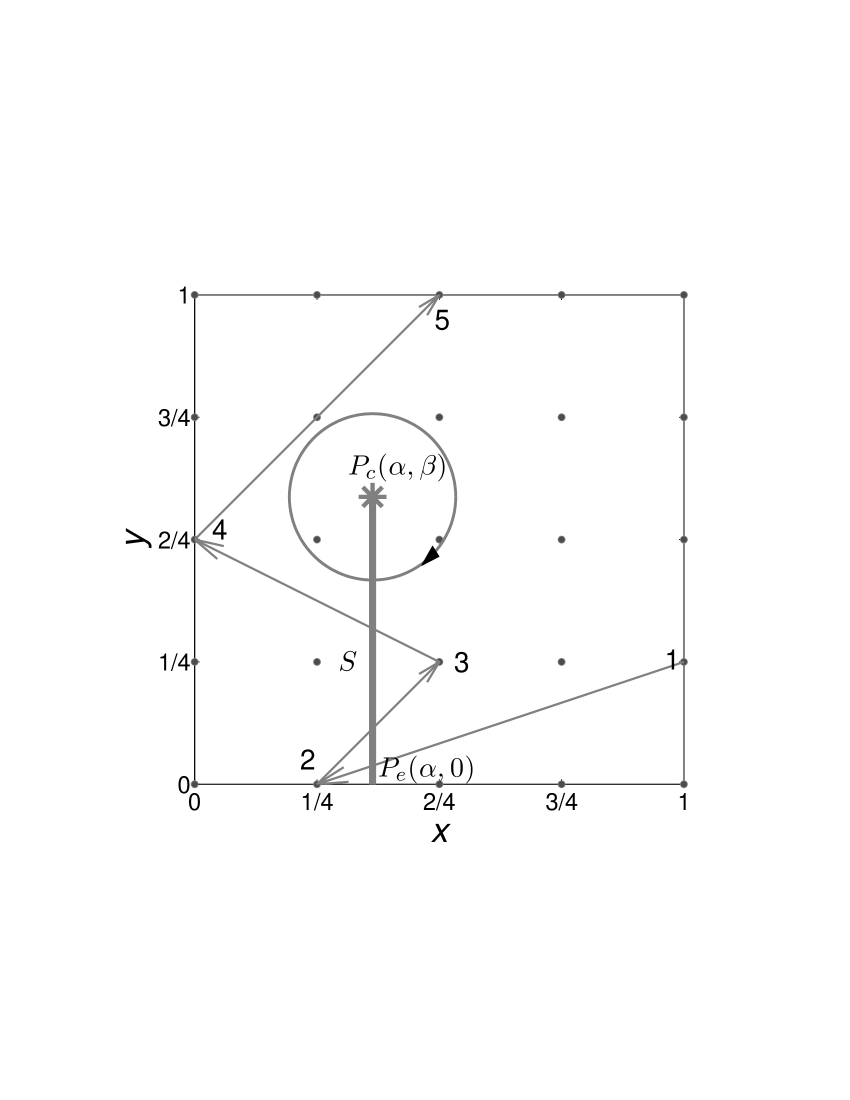
Figure 2: Schematic diagram for counting cycles Friedman2012 ; Xu20134997 . Background lattice represents the 25 social states. Including 4 transits, the successive segments (1 $\rightarrow$ 2 $\ldots$ $\rightarrow$ 5) form a trajectory of a social evolutionary transit path. The segment $S$ is the Poincare section (tripwire) from $P_{c}:=(\alpha,\beta)$ (star) to $P_{e}:=(\alpha,0)$ at the lower edge. In this paper, for each game, we set $(\alpha,\beta)$ at its Nash equilibrium ($x_{N},y_{N}$). For example, for Game-1, $(\alpha,\beta)=(0.91,0.09)$. The direction of the cycle surrounding the centre $(\alpha,\beta)$ is clockwise, as predicted by the two models.

3.2 Measurement of the frequency of the cycles

In this article, the experimental periodic frequency ($f_{exp}$) is defined as the time averaged net cycles counted in an experimental trajectory, which referring to Xu20134997 , is

$$f_{exp}=\frac{\sum_{i}C_{i}}{t_{1}-t_{0}},$$ (3)

where $\sum_{i}C_{i}$ is the accumulated counting number of cycles in time interval [$t_{0},t_{1}$] (the time unit in these 12 experiments is discrete in the experimental round), and $\bar{f}_{exp}$ is the average ${f}_{exp}$ over 12 groups of each of games 1 to 6 or 6 groups of each of games 7 to 12.

3.3 Measurement of the radius of the cycles

Whenever a transit-$i$ crosses the Poincare section, the Euclidean distance (denoted as $x_{i}$) between the crossing dot and the centre $N$ can be measured. Furthermore, for a given time interval $[t_{0},t_{1}]$, the average radius of the cycles can be defined as

$$R_{t_{0},t_{1}}=\frac{\sum_{i}x_{i}C_{i}}{\sum_{i}|C_{i}|}$$ (4)

where $i$ (=$1,2,3,\cdots$) denotes the $i$-th time that the trajectory passes the Poincare section. The sum covers all of the transits across the Poincare section. For example, according to Eq. 4, the radius of the net cycles ($R_{1,5}$) in Fig. 2 is -0.115. We use this measurement to evaluate the change in radius with time, which is necessary for cycle testing Nowak2012 ; Friedman2012 .

4 Results

As mentioned above (see Fig. 2 and the related text), we can illustrate the evolutionary trajectories of each group in the 12 experiments with the experimental data (see section 2.1). Accordingly, using the methods described in section 3, we can measure the experimental observations (accumulated number, frequency and radius of cycles) of the 12 experiments. Then, the experimental observations can be compared with the theoretical expectations (see section A.4) of the two different models. Results of statistical analysis are reported as follows.

4.1 Existence, persistence and direction of the cycles

Result 1: Cycles exist and persist, and the directions of net cycles in the “stochastic” trajectories meet the predictions of both evolutionary dynamics.

To test the existence of net cycles as in Xu20134997 , we calculate the average value $\bar{C}_{1,200}$ for the 12 games as well as the standard error of the mean (s.e.m) over the groups. The results are shown in Table 2. Using the Wilcoxon signed-rank test, we find that the $\bar{C}_{1,200}$ of all games are significantly less than 0, indicating the existence of cycles in all games except game 9, see Table 2. Using the 12 games as samples, we find that the existence of the net cycles is significant ($p$=$0.002$, Wilcoxon signed-rank test with $C_{1,200}=0$).

Table 2: Accumulated C, frequency and radius of the net cycles in the 12 experiments.

Game	Obs.♭	$\bar{C}_{1,200}$	$s.e.m^{\dagger}$	$p$-value‡	$\bar{f}_{exp}$	$s.e.m^{\dagger}$	$\bar{R}_{1,100}$	$\bar{R}_{101,200}$	$\bar{D}^{\S}$	$p$-value‡
1	12	-3.167	0.976	0.003	0.016	0.005	-0.035	-0.018	0.017	0.166
2	12	-4.000	1.142	0.013	0.020	0.006	-0.017	-0.026	-0.009	0.184
3	12	-2.750	0.789	0.006	0.014	0.004	-0.016	-0.010	0.006	0.386
4	12	-5.917	1.062	0.003	0.030	0.005	-0.017	-0.015	0.002	0.488
5	11	-8.167	1.160	0.002	0.041	0.006	-0.022	-0.024	-0.002	0.751
6	12	-10.083	1.311	0.002	0.051	0.007	-0.026	-0.020	0.006	0.204
7	6	-1.333	0.211	0.023	0.007	0.001	-0.014	0.000	0.014	0.423
8	6	-4.667	1.606	0.046	0.023	0.008	-0.017	-0.025	-0.008	0.423
9	6	-2.333	1.282	0.091	0.012	0.006	-0.010	-0.006	0.004	0.873
10	6	-6.333	1.745	0.027	0.032	0.009	-0.016	-0.016	0.000	0.522
11	6	-12.000	1.125	0.027	0.060	0.006	-0.024	-0.026	-0.001	0.749
12	6	-9.000	2.408	0.027	0.045	0.012	-0.021	-0.017	0.004	0.631

^♭: Number of groups. ^†: Standard error of the mean. ^‡: Wilcoxon signed-rank test, two-tailed. ^§: Average difference between $\bar{R}_{1,100}$ and $\bar{R}_{101,200}$ over 12 (6) groups.

The Wilcoxon signed-rank test verifies the persistence of cycles by comparing $C_{1,100}$ and $C_{101,200}$ of the 12 games. Results show that the null hypothesis: $C_{1,100}$=$C_{101,200}$ cannot be rejected ($p$=0.695, two-tailed, $d.f.$=11), which indicates the persistence of cycles.

Since all $\bar{C}_{1,200}$ of the 12 games are negative (see Table 2), the empirical directions of the cycles are clockwise statistically, consistent with the directions predicted by both of the two dynamics models as shown in Fig. 4.

4.2 Frequencies of the cycles

Result 2: The periodic frequency of the net cycles can be tested in data.

Before calculating the frequencies of cycles as in Xu20134997 , the number of cycles in the trajectory is counted. Fig. 3 presents the average number of the net cycles ($C_{1,t}$, see Eq. 2 for its explanation) along time $t$ ($t$ is up to 200 rounds in experiments, $t=200$) of each game. The 12 curves respectively represent the average cycles counted for the 12 experiments. For example, the red curve (Game 6) ends at about -10 at $t=200$. This indicates that in the 200-round game, about 10 cycles are counted on average over the 12 groups; meanwhile, the negative value implies the clockwise direction of the cycles.

The frequencies $f_{exp}$ of the 12 experiments are calculated according to Eq. 3. The results are shown in Table 2. The observed periodic frequencies of the 12 games are significantly different, which is consistent with the patterns of Fig. 3. Specifically, Eq. 3 indicates that the frequencies can be represented by the slopes of the $C_{1,200}$ curves in Fig. 3. Since the slopes are different for the 12 games, the frequencies are different.

In Section 5, we will show that the empirical frequencies of the cycles is an appropriate criterion for evaluating the models quantitatively.

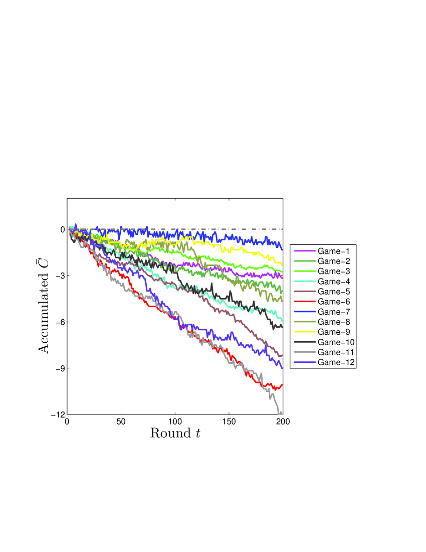
Figure 3: The dependence of the counted cycles on time. Each line is the average accumulated $C$ for one game. Negative values of the average accumulated $C_{1,t}$ indicate that the cycles are clockwise. Successive decline of the values indicates the persistence of cycles along time. The red curve reports the results of Game-6, in which the accumulated $\bar{C}$ is almost -10, indicating 10 clockwise cycles were obtained in 200 rounds and the frequency of cycles is about 0.05 (per round).

4.3 Change of the cycle radius over time

Result 3: The radius of the cycles does not change with time in the experiments, which supports the predictions of both of the two models.

For the 200-round experiments, our hypothesis is that the radius of the first 100 rounds ($R_{1,100}$) is equal to that of the second 100 rounds ($R_{101,200}$). The calculated results of $R_{1,100}$ and $R_{101,200}$ of the 12 games are shown in Table 2. Using the groups in each game as samples, the radius does not change in each of the 12 games ($p$-values are exhibited in Table 2, last column), and therefore the equal hypothesis cannot be significantly rejected. Using the 12 games as samples, we find that the equal hypothesis cannot be significantly rejected ($p=0.308$, Wilcoxon signed-rank test). Therefore, we can say that the statement that the radius does not change with respect to time is statistically supported.

5 Frequency as a criterion for model testing

As mentioned above, as a novel index, empirical frequencies of cycles could be employed to evaluate theoretical models quantitatively. We regress theoretical frequency ($f_{s}$ and $f_{a}$ in Table 1) on experimental frequencies ($\bar{f}_{exp}$ in Table 2) with the method of OLR and display the results in Table 3 (Appendix B provides details). These statistical results state that both of the models can interpret the differences among the observed frequencies quite well ($t>5$ in Table 3), while the adjusted model ($t$-value 6.41) performs slightly better.

In game theory, there exist tens of models known as population dynamics models (e.g., Weibull1997 ; Hofbauer2003 ; Sandholm2011 ; Castellano2009 ; szabo2007evolutionary ), finite population models (e.g., alos2003finite ; Traulsen2005 ; cremer2008anomalous ) or learning models (e.g.,  Camerer2003 ; RothComp2010 ). Comparisons between the models can be important Friedman2012 ; Xu20134997 , however since the main purpose of this paper is to report the definitive measurements in experiments, we do not extend our theoretical analysis to such comparisons. Nevertheless, the clear result ($t>5$ in Table 3) indicates that dynamic game models could be used effectively in combination with laboratory game experiments.

Table 3: OLR results of $\bar{f}_{exp}$ vs. $f_{s}$ and $f_{a}$ for the two models.

$\bar{f}_{exp}$	$Coef.$	$s.e.m$	$t$	$P>|t|$	[ 95%  C.I. ]
$f_{s}$	0.157	0.026	6.01	0.000	0.099  0.215
$\_cons$	-0.018	0.008	-2.16	0.056	-0.036  0.001
$f_{a}$	0.519	0.081	6.41	0.000	$~{}0.338~{}~{}0.699$
$\_cons$	0.001	0.005	0.25	0.805	$-0.010~{}~{}0.012$

6 Discussion and summary

First, in the 12 experimental $2\times 2$ games, we have confirmed the existence and persistence of the cycles, and the frequencies of cycles have been tested quantitatively. Furthermore, we have found that the observed periodic frequencies of the cycles are different when the games differ. Moreover, the experimental frequencies are linearly, positively and significantly related to the theoretical frequencies.

Experimental confirmation of social behaviour cycles is difficult benaim2009learning . Researchers continue to seek significant cyclic patterns to support evolutionary dynamics Friedman2012 ; Nowak2012 ; XuWang2011ICCS ; Xu20134997 . In some earlier works wang2012evolutionary , angular momentum was employed as an observable, but no periodic frequency was reported. In Ref. Friedman2012 , CRI was developed to index cycles, but once again no information was provided about periodic frequency Friedman2012 . In Ref. Xu20134997 , frequency served as an index for cycles, howeverthere is only one payoff matrix in their experiments, so that a quantitative comparison with theoretical frequencies is impossible. To the best of our knowledge, this paper is the first to report that cycles’ frequencies depend on the payoff matrices of the corresponding games.

We wish to emphasise our puzzles as follows. Even though the theoretical frequencies ($f_{s}$ and $f_{a}$) could meet experimental frequencies ($\bar{f}_{exp}$) well by OLR (see Table 3), we still hope to emphasise that such correspondence could be a coincidence, for example because the differences in the observed frequencies ($\bar{f}_{exp}$) could be interpreted by other factors, e.g., the distance ($D_{c}:=[(x_{N}-0.5)^{2}+(y_{N}-0.5)^{2}]^{\frac{1}{2}}$) from the centre of state space (0.5, 0.5) to the Nash Equilibrium ($x_{N},y_{N}$) of a game. For these 12 games, by OLR, there is a significant dependence of $\bar{f}_{exp}$ on $D_{c}$ ($t>5$) too, see Table 4. We are unaware of the reason for this significance. At the same time, we are unaware of why the coefficient in Table 3 differs significantly from 1. Admittedly, the relationship between games’ payoff matrix and empirical frequency is unclear. We hope to return to these issues in the future.

Table 4: OLR results of $\bar{f}_{exp}$ and the distance between the Nash Equilibrium and the centre of state space.

$\bar{f}_{exp}$	$Coef.$	$s.e.m$	$t$	$P>|t|$	[ 95%  C.I. ]
$D_{c}$	-0.104	0.017	-6.01	0.000	-0.142  -0.065
$\_cons$	0.067	0.007	9.92	0.000	0.052   0.082

In summary, we report the existence of persistent cycles, as well as their directions in $2\times 2$ games. Furthermore, the numerical frequencies of cycles are measured definitively and found to be significantly different across the 12 games (see $\bar{f}_{exp}$ in Table 2). We believe these empirical frequencies of cycles can be interpreted more precisely.

Acknowledgments: We, WZJ and XB, thank Hai-Jun Zhou for his critical comments and generous support on this work. We thank the anonymous reviewers for the helpful suggestions and Dr. Ekka for the excellent proofreading. We thank also Chuang Wang’s suggestions and Zunfeng Wang’s technical assistance. This work was supported by grants from the 985 Project at Zhejiang University (Project for experimental social science), SKLTP of ITPCAS (No. Y3KF261CJ1) and Philosophy $\&$ Social Sciences Planning Project of Zhejiang Province (13ND-JC095YB). Author Contributions: WZJ conceived research; WZJ and XB performed experimental analysis; WZJ and WS performed theoretical analysis; XB, WS and WZJ wrote the paper. After moved to Duke, WS did the language revision.

Appendix

Appendix A Theoretical predictions on cycles

Two versions of replicator dynamics, standard replicator dynamics and adjusted replicator dynamics, are used as references in the 12 experiments. As mentioned in main text, these parameter-free models are the most widely applied in both the economics and physics literature Traulsen2005 ; Maynard1982evolution ; Sandholm2011 ; Friedman1996 ; cremer2008anomalous ; Weibull1995evolutionary . Using the standard methods (e.g. Weibull1997 ; Sigmund1981 ), we can replicate the theoretical results on cycles.

A.1 Social states

In the view of evolutionary game theory Sandholm2011 , at each moment $t$, the consequence of social interaction can be described as a social state, which is a vector with the densities of strategies in each population as components. In the two-population game here, the strategy set for each player in the row population is (up, down) or $(X_{1}$,$X_{2})$ while for each player in the column population is (left, right) or $(Y_{1}$,$Y_{2})$. Let $p$ ($q$) denote the density of $X_{1}$ ($Y_{1}$) in the row (column) population, then $x$:=$(p,q)\in\mathbb{X}$ represents a social state, herein $\mathbb{X}$ is the social state space. Therefore, the state space is always a unit square as shown in Fig. 2.

Because there are four subjects in each population in this game, the social state space is $\mathbb{X}$=$\{0,\frac{1}{4},\frac{2}{4},\frac{3}{4},1\}\times\{0,\frac{1}{4},\frac{2}{4},\frac{3}{4},1\}$. That means, the actual full state space is a unit square of $5\times 5$ lattice points in which each social state can be represented by a lattice point, as shown in Fig. 2. For example, the social state 3 denoted as $x_{A}$=($\frac{2}{4},\frac{1}{4}$) is a state where $\frac{2}{4}$ of subjects in the first population choose $X_{1}$ and $\frac{1}{4}$ of subjects in the second population choose $Y_{1}$. It is clear that, at a given round (time) in an experiment, the social state can be observed Nowak2012 ; xu2012test ; XuWang2011ICCS ; Friedman2012 .

A.2 State-dependent payoff

There are a total of four possible strategies in the two populations. Suppose $x$ ($y$) is the proportion of the row (column) population using strategy $X_{1}$ ($Y_{1}$). It is natural that the density of strategy $X_{2}$ ($Y_{2}$) is $1-x$ ($1-y$). According to the payoff matrices of the games (see Table 1), the average payoff for the four strategies can be expressed as the following matrix:

$$\left[\begin{array}[]{c}U_{X_{1}}\\ U_{X_{2}}\\ U_{Y_{1}}\\ U_{Y_{2}}\end{array}\right]=\left[\begin{array}[]{c}a_{11}\,y+a_{12}\,\left(1-y\right)\\ a_{21}\,y+a_{22}\,\left(1-y\right)\\ b_{11}\,x+b_{21}\,\left(1-x\right)\\ b_{12}\,x+b_{22}\,\left(1-x\right)\end{array}\right]$$ (13)

where $U_{X_{i}}$ ($U_{Y_{i}}$), $i=1,2$ is the payoff for each player in the row (column) population choosing strategy $X_{i}$ ($Y_{i}$).

Further, the average payoff for each population can be aggregated as:

$$\left[\begin{array}[]{c}\bar{U}_{X}\\ \bar{U}_{Y}\end{array}\right]=\left[\begin{array}[]{c}x\,U_{X_{1}}+\left(1-x\right)\,U_{X_{2}}\\ y\,U_{Y_{1}}+\left(1-y\right)\,U_{Y_{2}}\end{array}\right].$$ (18)

Therefore, if the social state at $t$ is at $(x,y)$, according to the parameters of the payoff matrix of a given game, the average payoff for each strategy and the average payoff for each population can be calculated Sigmund1981 ; selten2008 .

A.3 Eigenvalues

To evaluate the cyclic social behaviours in the experimental games, we focus on the eigenvalues of the ordinary differential equations (ODE) of evolutionary dynamics. The systems are non-linear first-order differential equations. Mathematically, the eigenvalues, which are calculable, determine the dynamic properties of a system. To compare the experimental results with some earlier works Sigmund1981 ; Hofbauer1996 ; Maynard1982evolution ; Taylor1978 , we calculate the eigenvalues of the 12 games for the two dynamics.

A.3.1 Standard replicator dynamics

The ODE of the standard replicator dynamics is Taylor1978 ; Sigmund1981

$$\left\{\begin{array}[]{ccc}\dot{x}&=&~{}x(U_{X_{1}}-\bar{U}_{X})\\ \dot{y}&=&y(U_{Y_{1}}~{}-\bar{U}_{Y})\end{array}\right.$$ (21)

where ($x,y$) indicates a social state, $U$ and $\bar{U}$ have the same implications as in Eq. 13 and Eq. 18, respectively. The ODE describes how the social state changes according to the payoff of the strategies. For the $2\times 2$ games whose payoff matrices are shown as Fig. 1, according to Eq. 13 and Eq. 18, the ODE above can be presented as

$$\left\{\begin{array}[]{ccc}\dot{x}&=&-x\,\left(x-1\right)\cdot{}{}{}{}{}{}{}{}{}{}{}{}{}{}{}{}{}{}{}{}{}{}{}{}{}{}{}{}{}{}{}{}{}{}{}{}{}{}\\ &&\left(a_{12}-a_{22}+a_{11}\,y-a_{12}\,y-a_{21}\,y+a_{22}\,y\right)\\ \dot{y}&=&-y\,\left(y-1\right)\cdot{}{}{}{}{}{}{}{}{}{}{}{}{}{}{}{}{}{}{}{}{}{}{}{}{}{}{}{}{}{}{}{}{}{}{}{}{}{}\\ &&\left(b_{21}-b_{22}+b_{11}\,x-b_{12}\,x-b_{21}\,x+b_{22}\,x\right)\end{array}\right.$$ (26)

If we let $\dot{x}=0$ and $\dot{y}=0$, then there exists a unique inner Nash equilibrium of standard replicator dynamics ($N_{s}$) in the rectangular coordinate system constructed by $x$ and $y$ ($0<x,y<1$), which is

$$N_{s}=\left(\frac{b_{22}-b_{21}}{b_{11}-b_{12}-b_{21}+b_{22}},\frac{a_{22}-a_{12}}{a_{11}-a_{12}-a_{21}+a_{22}}\right)$$ (27)

We calculate the Nash equilibrium for the 12 games, denoted by ($x_{N},y_{N}$), as Table 1 shows. Then surrounding the $N_{s}$, the Jacobian is

$$J^{s}=\left[\begin{array}[]{cc}0&J_{12}^{s}\\ J_{21}^{s}&0\end{array}\right]$$ (28)

in which:

$$J_{12}^{s}=-\frac{\left(b_{11}-b_{12}\right)\,\left(b_{21}-b_{22}\right)\,\left(a_{11}-a_{12}-a_{21}+a_{22}\right)}{{\left(b_{11}-b_{12}-b_{21}+b_{22}\right)}^{2}}$$ (29)

and

$$J_{21}^{s}=-\frac{\left(a_{11}-a_{21}\right)\,\left(a_{12}-a_{22}\right)\,\left(b_{11}-b_{12}-b_{21}+b_{22}\right)}{{\left(a_{11}-a_{12}-a_{21}+a_{22}\right)}^{2}}$$ (30)

Then, the square of the eigenvalues of the Jacobian of the standard replicator dynamics, denoted as $\lambda_{s}^{2}$, is

$$\lambda_{s}^{2}=\frac{\left(a_{11}-a_{21}\right)\,\left(a_{12}-a_{22}\right)\,\left(b_{11}-b_{12}\right)\,\left(b_{21}-b_{22}\right)}{\left(a_{11}-a_{12}-a_{21}+a_{22}\right)\,\left(b_{11}-b_{12}-b_{21}+b_{22}\right)}$$ (31)

Plugging the payoff matrixes of the 12 games into Eq.31, we find that the squares of the eigenvalues are all negative, as shown in the $\lambda_{s}^{2}$ column in Table 1.

A.3.2 Adjusted replicator dynamics

The alternative version is called adjusted replicator dynamics (also called as payoff-normalised replicator dynamics in the economics literature) Traulsen2005 ; Weibull1997 ; Traulsen2009 ; Bowles2004 ; Sigmund2010 . Its ODE can be expressed as

$$\left\{\begin{array}[]{ccc}\dot{x}&=&x(U_{X_{1}}-\bar{U}_{X})\bar{U}_{X}^{-1}\\ \dot{y}&=&y(U_{Y_{1}}-\bar{U}_{Y})\bar{U}_{Y}^{-1}\end{array}\right.$$ (34)

Obviously, different to the replicator dynamics shown in Eq. 21, the item $\bar{U}_{X}^{-1}$ and $\bar{U}_{Y}^{-1}$ in Eq. 34 make the payoffs normalised. Specified for $2\times 2$ games whose payoff matrices are shown in Fig. 1, according to Eq. 13 and Eq. 18, the ODE of the adjusted replicator dynamics can be presented as

$$\left\{\begin{array}[]{ccc}\dot{x}&=&x\left(1-x\right)\left[\left(a_{12}-a_{22}\right)+Ay\right]\cdot{}{}{}{}{}{}{}{}{}{}{}{}{}{}{}{}{}{}{}{}{}\\ &&[Axy+(a_{12}-a_{22})x+(a_{21}-a_{22})y+a_{22}]^{-1}\\ \dot{y}&=&y\left(1-y\right)\left[\left(b_{21}-b_{22}\right)+Bx\right]\cdot{}{}{}{}{}{}{}{}{}{}{}{}{}{}{}{}{}{}{}{}{}\\ &&[Bxy+(b_{21}-b_{22})y+(b_{12}-b_{22})x+b_{22}]^{-1}\end{array}\right.$$ (39)

where we have introduced the short hand $A=a_{11}-a_{21}+a_{22}-a_{12}$ and $B=b_{11}-b_{12}+b_{22}-b_{21}$.

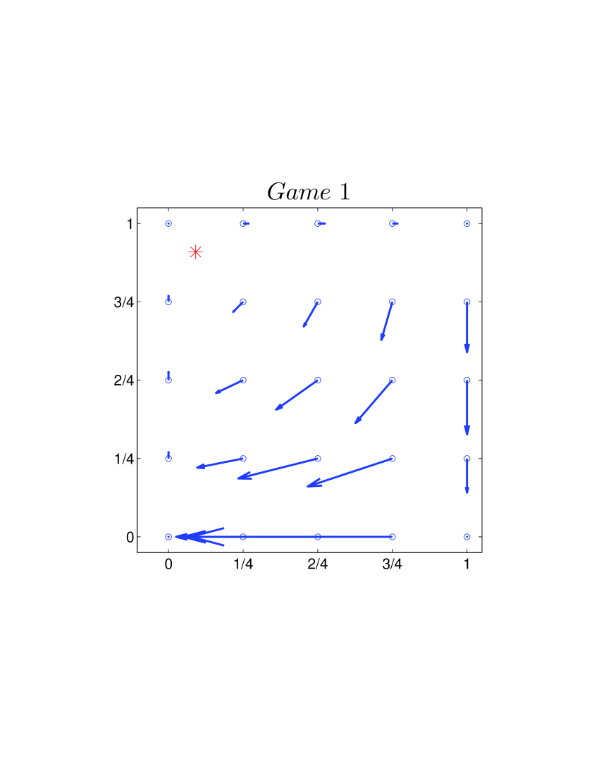
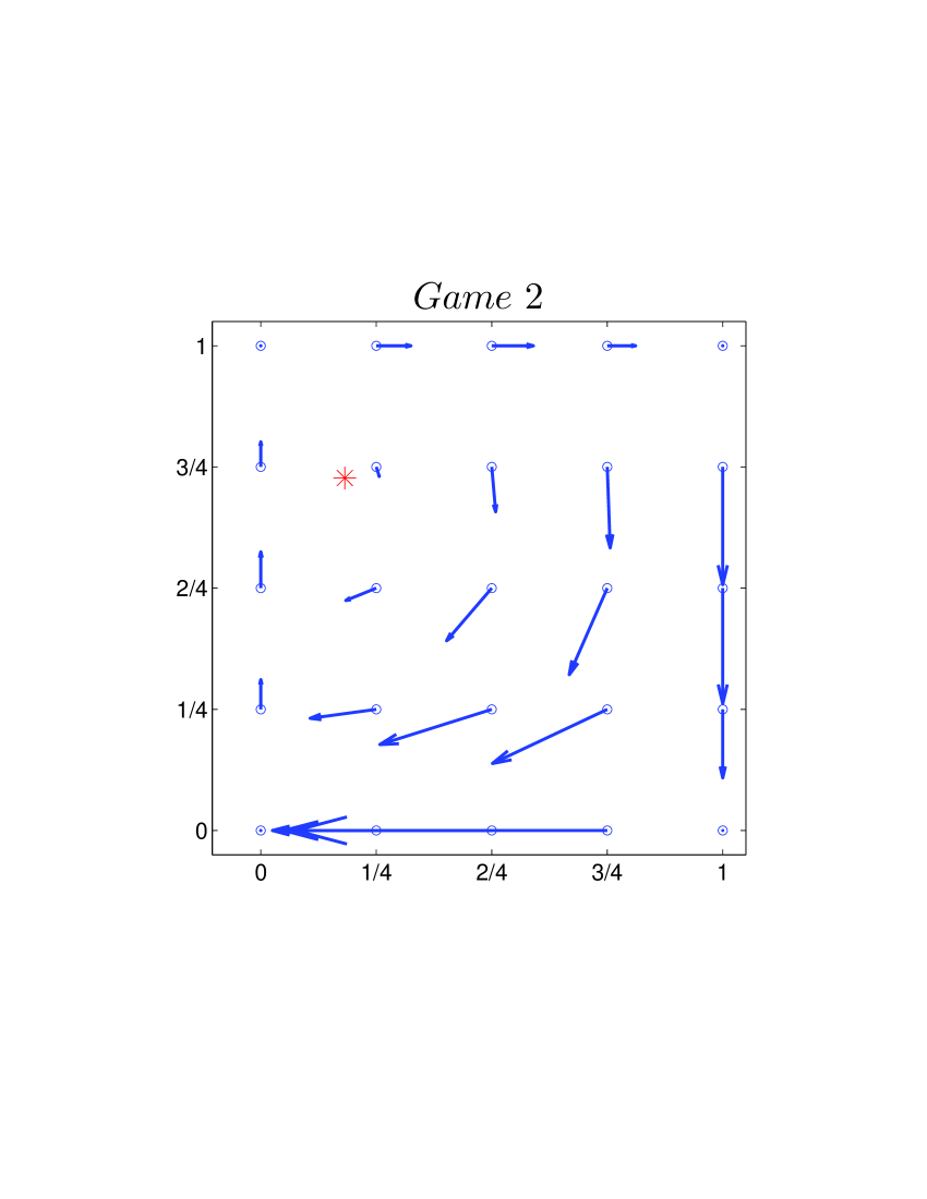
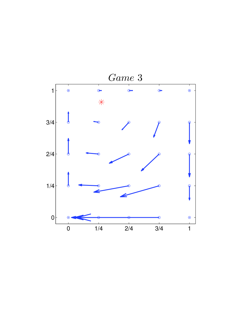
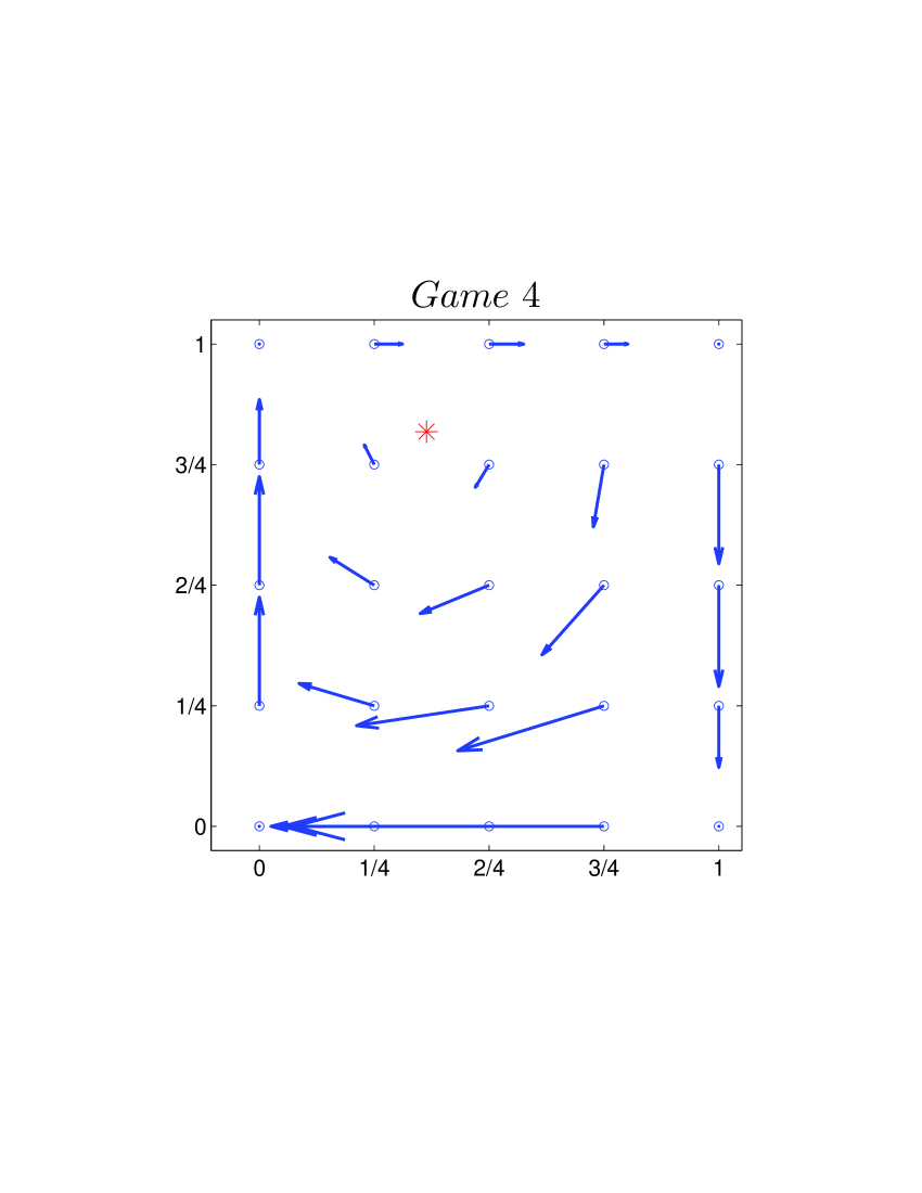
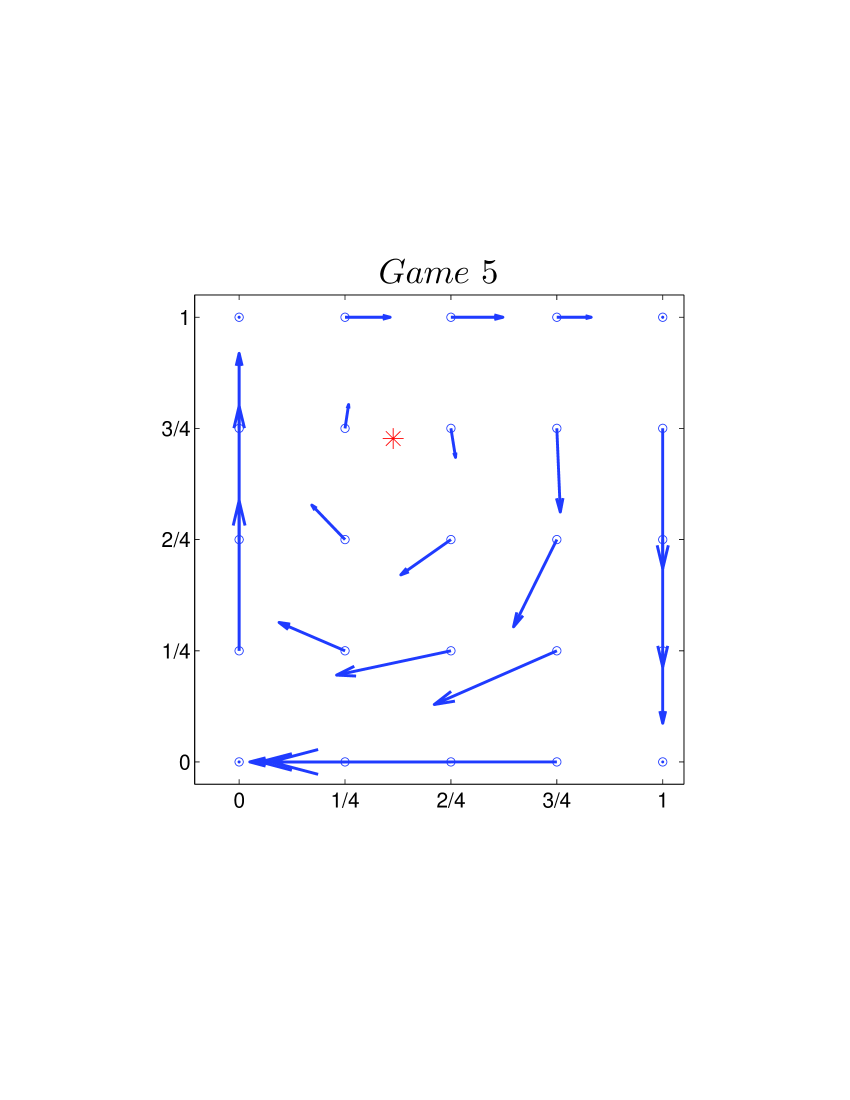
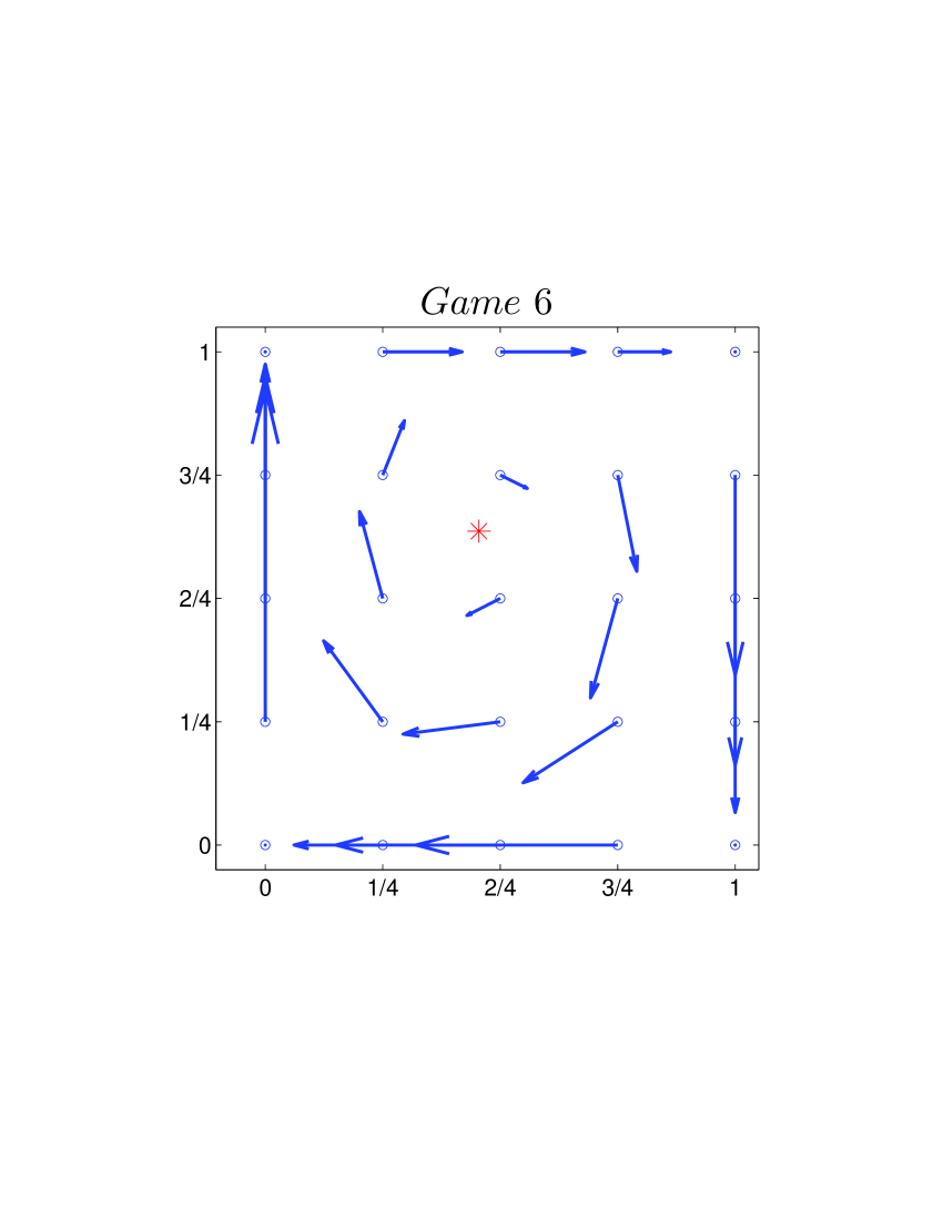
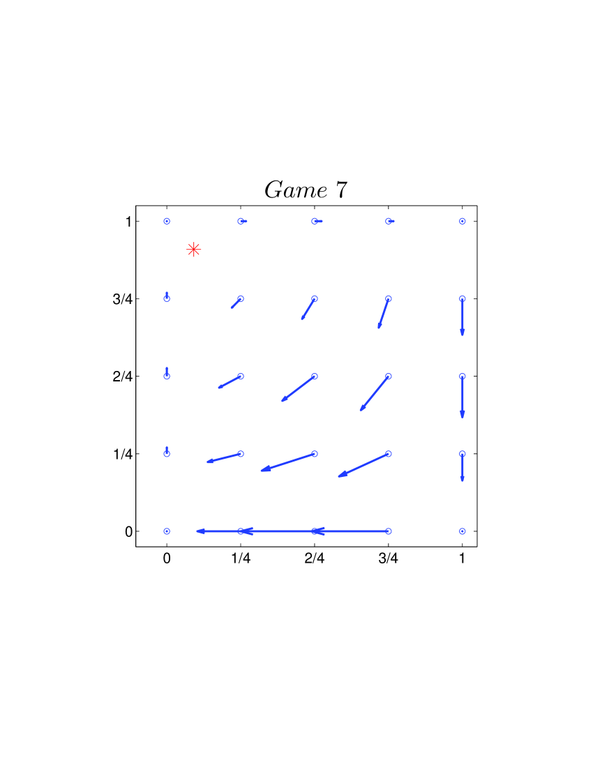
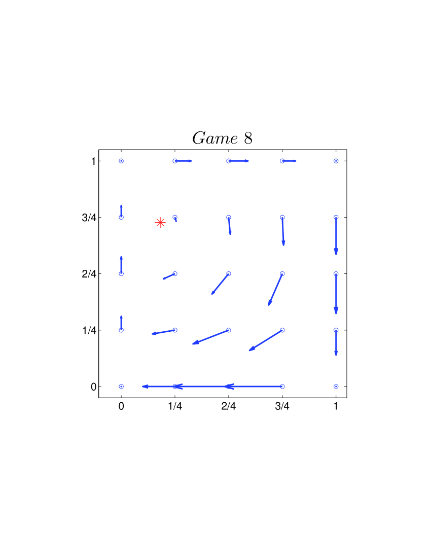
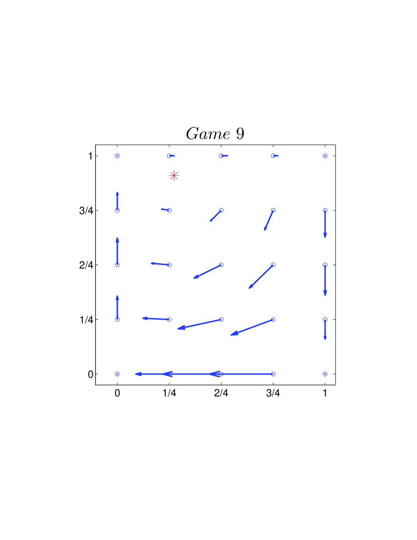
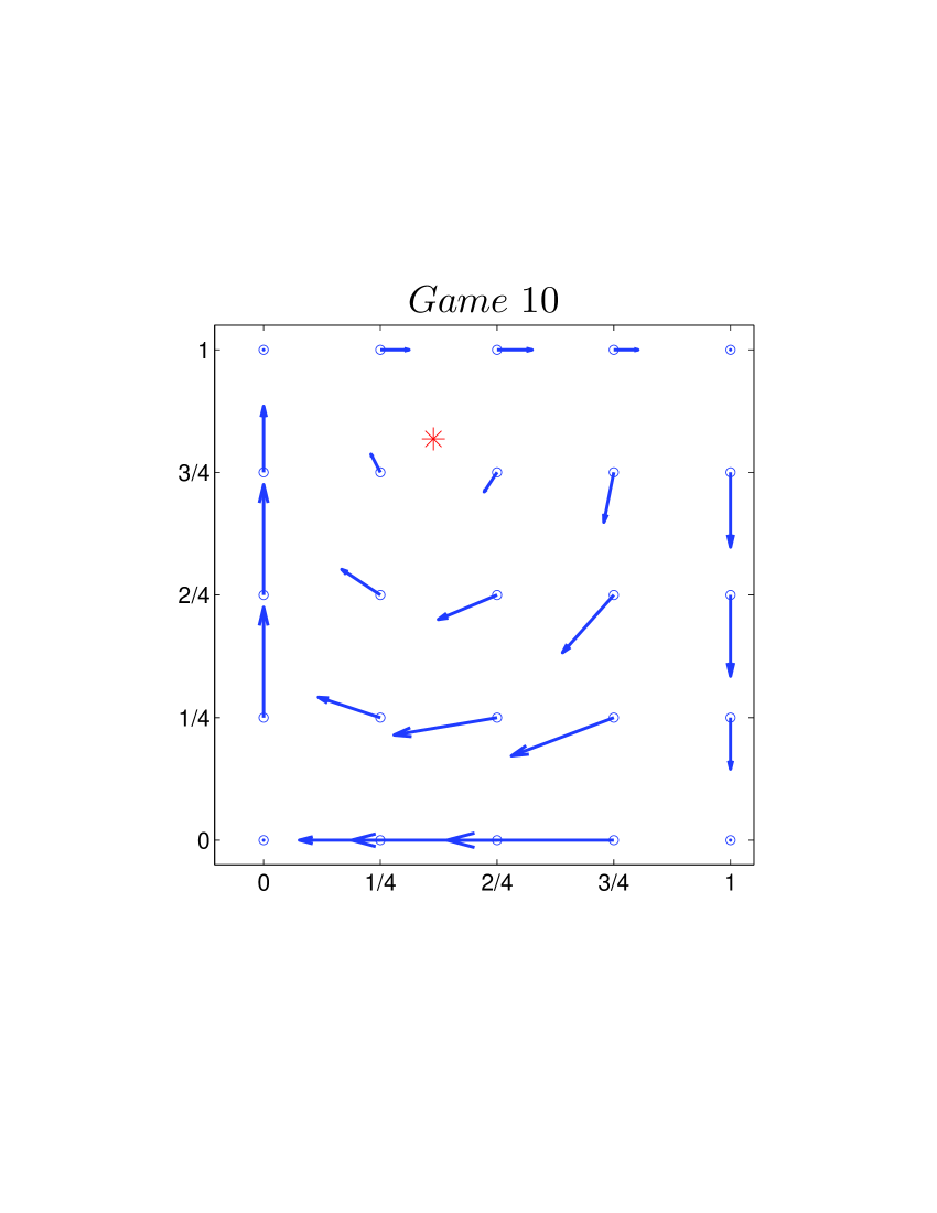
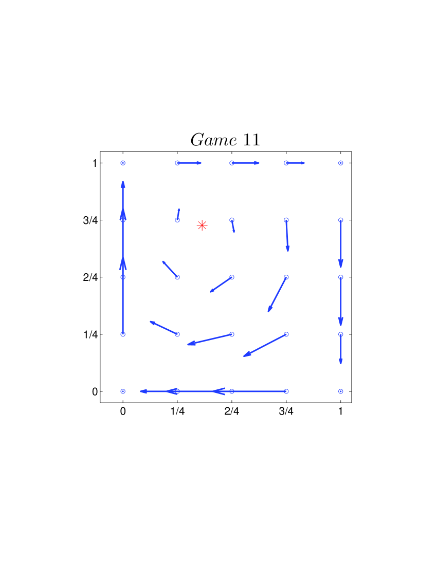
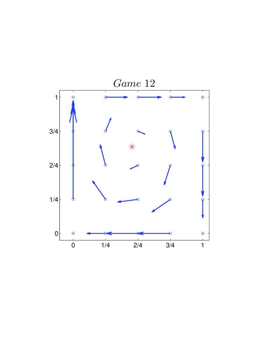
Figure 4: The expected velocity field of the adjusted replicator dynamics. The arrow of the vector at each site represents the direction of the transit. The magnitude of the vector at each site represents the strength of the transit. At the 25 observable states, a two dimensional vector can be plotted with Eq. 39 and the payoff matrix elements in Table 1. Surrounding the Nash equilibrium point (red cross), all of the global patterns of the 12 games are of clockwise.

For adjusted replicator dynamics, there also exists a unique inner Nash equilibrium $N_{a}$ in the rectangular coordinate system constructed by $x$ and $y$ ($0<x,y<1$), which is

$$N_{a}=\left(\frac{b_{21}-b_{22}}{b_{21}-b_{22}+b_{12}-b_{11}},\frac{a_{12}-a_{22}}{a_{12}-a_{22}+a_{21}-a_{11}}\right).$$ (40)

As $N_{a}$ in Eq. 40 is equal to $N_{s}$ in Eq. 27, we have the result that the Nash equilibria of the two models are identical.

Again, surrounding the equilibrium point $N_{a}$, the Jacobian of Eq. 39 is

$$J^{a}=\left[\begin{array}[]{cc}0&J_{12}^{a}\\ J_{21}^{a}&0\end{array}\right].$$ (41)

in which:

$$J_{12}^{a}=\frac{(b_{11}-b_{12})(b_{21}-b_{22})(a_{12}-a_{22}+a_{21}-a_{11})^{2}}{(a_{12}a_{21}-a_{11}a_{22})(b_{21}-b_{22}+b_{12}-b_{11})^{2}}$$ (42)

and

$$J_{21}^{a}=\frac{(a_{11}-a_{21})(a_{12}-a_{22})(b_{21}-b_{22}+b_{12}-b_{11})^{2}}{(b_{21}b_{12}-b_{11}b_{22})(a_{12}-a_{22}+a_{21}-a_{11})^{2}}.$$ (43)

Then, the square of the eigenvalues of the Jacobian of the adjusted replicator dynamics, denoted as $\lambda_{a}^{2}$, is

$$\lambda_{a}^{2}=\frac{\left(a_{11}-a_{21}\right)\left(a_{12}-a_{22}\right)\left(b_{11}-b_{12}\right)\left(b_{21}-b_{22}\right)}{\left(a_{12}\,a_{21}-a_{11}\,a_{22}\right)\left(b_{21}\,b_{12}-b_{11}\,b_{22}\right)}$$ (44)

For the 12 games, the results of $\lambda_{a}^{2}$ are shown in Table 1.

One point worth emphasising is that since all the $\lambda^{2}$ are negative, the eigenvalues should be purely imaginary. So, the solution of the dynamics (Eq. 26 and Eq. 39 near Nash equilibrium) is cyclic and equivalent to simple harmonic motion (SHM). The following part explains this point in more detail.

We use $(\triangle x,\triangle y)$ to present the deviation from the Nash Equilibrium of $(x,y)$. Referring to the Jacobian (Eq. 41 for adjusted replicator dynamics), we have

$$\left[\begin{array}[]{c}\dot{\triangle x}\\ \dot{\triangle y}\end{array}\right]=\left[\begin{array}[]{cc}0&J_{12}^{a}\\ J_{21}^{a}&0\end{array}\right]\left[\begin{array}[]{c}\triangle x\\ \triangle y\end{array}\right].\\$$ (45)

From time derivation of this equation, we have

$$\left[\begin{array}[]{c}\ddot{\triangle x}\\ \ddot{\triangle y}\end{array}\right]=\left[\begin{array}[]{cc}J_{12}^{a}J_{21}^{a}&0\\ 0&J_{12}^{a}J_{21}^{a}\end{array}\right]\left[\begin{array}[]{c}\triangle x\\ \triangle y\end{array}\right].\\$$ (46)

Mathematically, this dynamics is equivalent to asymmetric games with cyclic dynamics (see Eq. J. 3 in Appendixes J in textbook Maynard1982evolution ) and the solutions of this dynamics are closed cyclical orbits.

A.4 Theoretical expectations

The theoretical expectations of directions, frequencies and changes in radius of the cycles can be obtained from the eigenvalues (in Eq. 31 and Eq. 44) as well as the Jacobian (in Eq. 28 and Eq. 41).

A.4.1 Directions of cycles

In state space, the direction of cycles could be clockwise or counter-clockwise. We use two methods to evaluate it.

One way is to plot the velocity field on the basis of Eq. 26 and Eq. 39. As shown in Fig. 4, all directions of the velocity fields are clockwise. Another way is using the Jacobian described Sigmund1981 before. Calculating the Jacobian (Eq. 28 or Eq. 41) explicitly, we can get the changing direction at each given state around $N_{s}$ (or $N_{a}$). For the two dynamics, as $J_{12}>0$ and $J_{21}<0$ hold for all the 12 games, we have all the directions in a clockwise manner.

At the same time, it also explains the existence and persistence of the cycles in the same ways.

A.4.2 Frequencies of cycles

As mentioned above, the eigenvalue $\lambda$ (denoted as $\lambda=\alpha\pm i\beta$) of the 12 games is purely imaginary, i.e. the real part ($\alpha$) is zero for all $\lambda$. Mathematically, the motion is equivalent to SHM, in which the value of $\beta$ refers to the angular frequency (also called angular speed, see page 199 in holzner2011physics ). Since there are 2$\pi$ radians in one cycle, in order to complete the cycle $2\pi/\beta$ units of time are needed. So the theoretical periodic frequency ($f_{theo}$) is explicitly given as:

$$f_{theo}=\frac{\beta}{2\pi}$$ (47)

For the 12 games, the values of $f_{theo}$ for standard and adjusted replicator dynamics (denoted as $f_{s}$ and $f_{a}$, respectively) are different (shown in Table 1). They will serve as the theoretical expectations (in Table 3 and Fig. 5) to be compared with observed frequencies.

A.4.3 Radius of cycles

As noted, for all of the 12 games and both of the models, the real parts of the eigenvalues ($\alpha$) are equal to 0. As mentioned above, motions of these game systems are mathematically equivalent to simple harmonic motion. Since $\alpha=0$, the radius of cycles does not change with time.

In the 200-round experiments, the testable hypothesis is: the cycle radius of the first 100 rounds equals that of the second 100 rounds.

Appendix B Evaluation of the two replicator dynamics

This part is the supporting material for Table 3. The statistic method and the comparison results are explained as follows.

B.1 Statistic method

Referring to the theoretical frequency ($f_{s}$ and $f_{a}$ in Table 1) and the experimental frequencies ($\bar{f}_{exp}$ in Table 2), the OLR results are shown in Table 3. The relationship between the theoretical frequencies ($f_{theo}$) and experimental frequencies ($\bar{f}_{exp}$) of the 12 games can also be demonstrated as in Fig. 5. The statistical testing and analysis are explained as follows.

(1) For the comparison with $f_{s}$ from the standard replicate dynamics, statistical results show that the coefficient of the linear regression over the 12 paired samples is $0.157\pm 0.026$. It indicates that the positive correlation between theoretical frequencies and experimental frequencies is strongly significant (at $t>5$ level). In addition, the constant of the regression is $-0.018\pm 0.008$ ($p=0.056>0.05$) and its $95\%$ C.I. [-0.036 0.shi001] includes zero. This implies that there is no systematic deviation.

(2) Comparing with $f_{a}$ from the adjusted replicate dynamics, statistical results show that the coefficient of the linear regression over the 12 paired samples is $0.519\pm 0.081$. This indicates that the positive correlation between theoretical frequencies and experimental frequencies is strongly significant (at $t=6.41>5$ level). In addition, the constant of the regression is $0.001\pm 0.005$ ($p=0.805$, two-tailed) and its $95\%$ C.I. [-0.010 0.012] includes 0.000. This implies that there is no systematic deviation here either.

B.2 Comparison results

The comparison results are as follows.

(1) According to the $p$-value of the coefficient of the linear regression, both of the models’ expectations are positively related to experimental observations, and can infer the difference of the observed frequencies well. Since the constant is closer to 0 and the $t$-value (see Table 3) is larger, the adjusted replicator dynamics therefore performs better.

(2) However, neither of the two models can capture the observed frequencies quantitatively and exactly, because the values of the coefficients of the linear regression for both the standard replicator dynamics ($0.157\pm 0.026$) and the adjusted replicator dynamics ($0.519\pm 0.081$) are significantly different from 1.

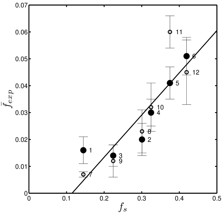
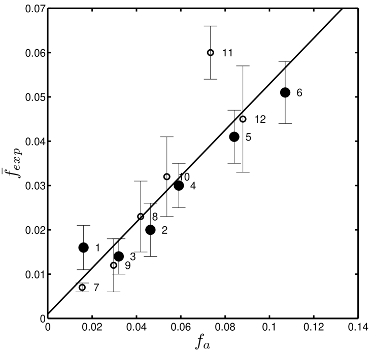
Figure 5: The relationship between empirical frequencies and theoretical frequencies. The $x$-axis ($y$-axis) indicates the theoretical frequency $f_{theo}$ (the experimental frequency $\bar{f}_{exp}$). The $f_{s}$ in the panel above comes from standard replicator dynamics, and the $f_{a}$ in the panel below is from adjusted replicator dynamics. The black dots indicate the mean of each 12-group game (games 1 to 6) and the black holes of each 6-group game (games 7 to 12). The bars indicate the s.e.m (standard error of the mean) and the numbers correspond to the game ID. The slope lines are plotted according to the results of OLR. The adjusted replicator dynamics perform significantly better than the standard replicator dynamics.

References

- (1) J. Von Neumann, O. Morgenstern, Theory of Games and Economic Behavior (Princeton university press, 1944)
- (2) J. Smith, Evolution and the Theory of Games (Cambridge university press, 1982)
- (3) B. Andrae, J. Cremer, T. Reichenbach, et al., Physical Review Letters 104, 21, 218102 (2010)
- (4) R. Myerson, Game Theory: Analysis of Conflict (Harvard Univ Pr, 1997)
- (5) R. Dawkins, The Selfish Gene. 1976 (1976)
- (6) P. Schuster, K. Sigmund, Animal Behaviour 29, 1, 186 (1981)
- (7) J. Cremer, T. Reichenbach, E. Frey, The European Physical Journal B 63, 3, 373 (2008)
- (8) J. C. Claussen, The European Physical Journal B 60, 3, 391 (2007)
- (9) P. Taylor, L. Jonker, Mathematical Biosciences 40, 1-2, 145 (1978)
- (10) J. Weibull, Evolutionary Game Theory (The MIT press, 1997)
- (11) J. Hofbauer, K. Sigmund, Bulletin of the American Mathematical Society 40, 4, 479 (2003)
- (12) W. Sandholm, Population Games And Evolutionary Dynamics (MIT press, 2011)
- (13) A. Falk, J. Heckman, Science 326, 5952, 535 (2009)
- (14) L. Samuelson, The Journal of Economic Perspectives 16, 2, 47 (2002)
- (15) K. Binmore, J. Swierzbinski, C. Proulx, The Economic Journal 111, 473, 445 (2001)
- (16) D. Friedman, The Economic Journal 106, 434, 1 (1996)za
- (17) C. Anderson, C. Plott, K. Shimomura, et al., Journal of Economic Theory 115, 2, 209 (2004)
- (18) T. N. Cason, D. Friedman, E. Hopkins, The Review of Economic Studies 81, 112 (2014)
- (19) B. Xu, H.-J. Zhou, Z. Wang, Physica A: Statistical Mechanics and its Applications 392, 20, 4997 (2013)
- (20) R. Selten, T. Chmura, The American Economic Review 98, 938 (2008)
- (21) A. Traulsen, J. Claussen, C. Hauert, Physical Review Letters 95, 23, 238701 (2005)
- (22) M. Hoffman, S. Suetens, M. A. Nowak, et al., (unpublished) (2012)
- (23) T. Borgers, R. Sarin, Journal of Economic Theory 77, 1, 1 (1997)
- (24) Y. Cheung, D. Friedman, Journal of Economic Behavior and Organization 35, 3, 263 (1998)
- (25) B. Xu, Z. Wang, in Unifying Themes in Complex Systems Volume VIII, edit by H. Sayama, A. Minai, D. Braha, et al. (NECSI Knowledge Press, ISBN 978-0-9656328-4-3, 2011), p. 1313
- (26) H. P. Young, Stochastic Adaptive Dynamics (Palgrave Macmillan, Basingstoke, 2008)
- (27) S. Dorosz, M. Pleimling, Physical Review E 83, 3, 031107 (2011)
- (28) B. Xu, Z. Wang, SSRN eLibrary, Social Transition Spectrum in Constant Sum 2x2 Games with Human Subjects, http://dx.doi.org/10.2139/ssrn.1910045 (2011)
- (29) C. Castellano, V. Loreto, Reviews of Modern Physics 81, 2, 591 (2009)
- (30) G. Szabó, G. Fáth, Physics Reports 446, 4, 97 (2007)
- (31) C. Alós-Ferrer, International Game Theory Review 5, 03, 263 (2003)
- (32) C. Camerer, R. S. Foundation, Behavioral Game Theory: Experiments in Strategic Interaction, vol. 9 (Princeton University Press Princeton, NJ, 2003)
- (33) I. Erev, E. Ert, A. Roth, et al., Journal of Behavioral Decision Making 23, 1, 15 (2010)
- (34) M. Benaīm, J. Hofbauer, E. Hopkins, Journal of Economic Theory 144, 4, 1694 (2009)
- (35) Z. Wang, B. Xu, arXiv preprint arXiv:1203.2591 (2012)
- (36) K. Ritzberger, J. Weibull, Econometrica: Journal of the Econometric Society 1371–1399 (1995)
- (37) B. Xu, Z. Wang, Results in Physics 2, 0, 127 (2012)
- (38) J. Hofbauer, Journal of mathematical biology 34, 5, 675 (1996)
- (39) A. Traulsen, C. Hauert, Reviews of Nonlinear Dynamics and Complexity 2, 25 (2009)
- (40) S. Bowles, Microeconomics: Behavior, Institutions, and Evolution (Princeton University Press, 2004)
- (41) K. Sigmund, The Calculus of Selfishness (Princeton Univ Pr, 2010)
- (42) S. Holzner, Physics I for Dummies (For Dummies, 2011)