Nikhef-2012-012

Exploring $B_{s}\to D_{s}^{(*)\pm}K^{\mp}$ Decays in the
Presence of a Sizable Width Difference $\Delta\Gamma_{s}$

Kristof De Bruyn ^a, Robert Fleischer ^a,b, Robert Knegjens ^a,
Marcel Merk ^a,b, Manuel Schiller ^a and Niels Tuning ^a

^aNikhef, Science Park 105, NL-1098 XG Amsterdam, Netherlands

^bDepartment of Physics and Astronomy, Vrije Universiteit Amsterdam,
NL-1081 HV Amsterdam, Netherlands

The $B_{s}\to D_{s}^{(*)\pm}K^{\mp}$ decays allow a theoretically clean determination of $\phi_{s}+\gamma$, where $\phi_{s}$ is the $B^{0}_{s}$–$\bar{B}^{0}_{s}$ mixing phase and $\gamma$ the usual angle of the unitarity triangle. A sizable $B_{s}$ decay width difference $\Delta\Gamma_{s}$ was recently established, which leads to subtleties in analyses of the $B_{s}\to D_{s}^{(*)\pm}K^{\mp}$ branching ratios but also offers new “untagged” observables, which do not require a distinction between initially present $B^{0}_{s}$ or $\bar{B}^{0}_{s}$ mesons. We clarify these effects and address recent measurements of the ratio of the $B_{s}\to D_{s}^{\pm}K^{\mp}$, $B_{s}\to D_{s}^{\pm}\pi^{\mp}$ branching ratios. In anticipation of future LHCb analyses, we apply the $SU(3)$ flavour symmetry of strong interactions to convert the $B$-factory data for $B_{d}\to D^{(*)\pm}\pi^{\mp}$, $B_{d}\to D_{s}^{\pm}\pi^{\mp}$ decays into predictions of the $B_{s}\to D_{s}^{(*)\pm}K^{\mp}$ observables, and discuss strategies for the extraction of $\phi_{s}+\gamma$, with a special focus on untagged observables and the resolution of discrete ambiguities. Using our theoretical predictions as a guideline, we make simulations to estimate experimental sensitivities, and extrapolate to the end of the planned LHCb upgrade. We find that the interplay between the untagged observables, which are accessible thanks to the sizable $\Delta\Gamma_{s}$, and the mixing-induced CP asymmetries, which require tagging, will play the key role for the experimental determination of $\phi_{s}+\gamma$.

August 2012

1 Introduction

The decays $B_{s}\to D_{s}^{(*)\pm}K^{\mp}$ only receive contributions from tree-diagram-like topologies. Since both $B^{0}_{s}$ and $\bar{B}^{0}_{s}$ mesons can decay into the $D_{s}^{(*)\pm}K^{\mp}$ final states, interference effects between $B^{0}_{s}$–$\bar{B}^{0}_{s}$ mixing and decay processes allow a theoretically clean determination of the CP-violating phase $\phi_{s}+\gamma$ [1, 2], where $\phi_{s}$ is the $B^{0}_{s}$–$\bar{B}^{0}_{s}$ mixing phase and $\gamma$ the corresponding angle of the unitarity triangle. As $\phi_{s}$ can be extracted separately, with the latest experimental average given by [3]

$$\phi_{s}=\left(-2.5^{+5.2}_{-4.9}\right)^{\circ},$$ (1)

$\gamma$ can be determined.

The central question is then whether this value will agree with $\gamma$ determinations from decays with penguin contributions, such as the $B^{0}_{d}\to\pi^{+}\pi^{-}$, $B^{0}_{s}\to K^{+}K^{-}$ system [4]. The current picture of direct determinations of $\gamma$ from tree decays can be summarized as follows:

$$\gamma=\left\{\begin{array}[]{ll}(66\pm 12)^{\circ}&\mbox{(CKMfitter Collaboration \cite[cite]{[\@@bibref{}{CKMfitter}{}{}]})}\\ (76\pm 10)^{\circ}&(\mbox{UTfit Collaboration \cite[cite]{[\@@bibref{}{UTfit}{}{}]}}).\end{array}\right.$$ (2)

On the other hand, a recent analysis of the $B^{0}_{d}\to\pi^{+}\pi^{-}$, $B^{0}_{s}\to K^{+}K^{-}$ system gives

$$\gamma=(68\pm 7)^{\circ},$$ (3)

where the error also takes $SU(3)$-breaking corrections into account [7].

In the present paper, we assume that the relevant decay amplitudes are described by the Standard Model (SM). Applying the formalism developed in Ref. [2], we shall explore the $B_{s}\to D_{s}^{(*)\pm}K^{\mp}$ channels both in view of recent experimental developments and measurements to be performed by the LHCb collaboration in this decade.

Using the $B^{0}_{s}\to J/\psi\phi$ channel, the LHCb experiment has recently established a non-vanishing decay width difference of the $B_{s}$-meson system, which is characterized by the following parameter [8]:

$$y_{s}\equiv\frac{\Delta\Gamma_{s}}{2\,\Gamma_{s}}\equiv\frac{\Gamma_{\rm L}^{(s)}-\Gamma_{\rm H}^{(s)}}{2\,\Gamma_{s}}=0.088\pm 0.014.$$ (4)

Here $\tau_{B_{s}}^{-1}\equiv\Gamma_{s}\equiv\bigl{[}\Gamma_{\rm L}^{(s)}+\Gamma_{\rm H}^{(s)}\bigr{]}/2=\left(0.6580\pm 0.0085\right)\mbox{ps}^{-1}$ [8] denotes the inverse of the $B_{s}$ mean lifetime $\tau_{B_{s}}$. A discrete ambiguity could also be resolved [9], thereby leaving us with the sign of $\Delta\Gamma_{s}$ in (4), which is in agreement with the SM expectation (for a recent review, see [10]).

This new development in the exploration of the $B_{s}$-meson system has important consequences:

• Untagged $B_{s}$ decay data samples, where no distinction is made between initially, i.e. at time $t=0$, present $B^{0}_{s}$ or $\bar{B}^{0}_{s}$ mesons, allow for an extraction of interesting observables [2].

• A subtle difference arises between the branching ratios extracted experimentally, and those usually considered by theory [11].

First measurements of the $B_{s}\to D_{s}^{\pm}K^{\mp}$ branching ratios are available from the CDF [12], Belle [13] and LHCb [14] collaborations:

$$\frac{\text{BR}(B_{s}\rightarrow D_{s}^{\pm}K^{\mp})_{\rm exp}}{\text{BR}(B_{s}\rightarrow D_{s}^{\pm}\pi^{\mp})_{\rm exp}}=\left\{\begin{array}[]{lcl}0.097\pm 0.018\>(\text{stat.})\pm 0.009\>(\text{syst.})&&{\rm[CDF],}\\ 0.065^{+0.035}_{-0.029}\>(\text{stat.})&&{\rm[Belle],}\\ 0.0646\pm 0.0043\>(\text{stat.})\pm 0.0025\>(\text{syst.})&&{\rm[LHCb];}\end{array}\right.$$ (5)

the errors of the Belle result are dominated by the small $B_{s}\rightarrow D_{s}^{\pm}K^{\mp}$ data sample. We shall clarify the impact of $\Delta\Gamma_{s}$ on this ratio of CP-averaged experimental branching ratios and convert the experimental numbers into constraints on the hadronic parameter characterizing the interference effects discussed above.

As was pointed out in Ref. [2], the observables of the $B_{s}\to D_{s}^{(*)\pm}K^{\mp}$ channels can be related to those of the $B_{d}\to D^{(*)\pm}\pi^{\mp}$ decays through the $U$-spin symmetry of strong interactions. We shall use $B$-factory data for the latter decays obtained by the BaBar and Belle collaborations, with further constraints from $B_{d}\to D_{s}^{\pm}\pi^{\mp}$ modes, to make predictions for the $B_{s}\to D_{s}^{(*)\pm}K^{\mp}$ observables that will serve as a guideline for the expected experimental picture. In this analysis, we specifically find that – thanks to the sizable value of $\Delta\Gamma_{s}$ – untagged data samples of $B_{s}\to D_{s}^{(*)\pm}K^{\mp}$ decays can be efficiently combined with mixing-induced CP asymmetries of tagged analyses to extract $\phi_{s}+\gamma$ in an unambiguous way.

The outline is as follows: in Section 2, we discuss untagged measurements of the $B_{s}\to D_{s}^{(*)\pm}K^{\mp}$ decays and their effective lifetimes, addressing also the results listed in (5). In Section 3, we apply $SU(3)$ flavour symmetry to extract the hadronic parameters characterizing the $B_{s}\to D_{s}^{(*)\pm}K^{\mp}$ decays from the $B$-factory data for the $B_{d}\to D^{(*)\pm}\pi^{\mp}$ and $B_{d}\to D_{s}^{\pm}\pi^{\mp}$ channels. In Section 4, we discuss the extraction of $\phi_{s}+\gamma$ from the tagged and untagged $B_{s}\to D_{s}^{(*)\pm}K^{\mp}$ observables, with a special emphasis on resolving the discrete ambiguities. The hadronic parameters obtained in Section 3 are used in Section 5 to predict the relevant $B_{s}\to D_{s}^{(*)\pm}K^{\mp}$ observables, which then serve as an input for exploring the experimental prospects. Finally, we summarize our conclusions in Section 6.

2 Untagged Observables

The time-dependent, untagged $B_{s}\to D_{s}^{(*)+}K^{-}$ decay rates can be written as follows [2]:

$$\langle\Gamma(B_{s}(t)\to D_{s}^{(*)+}K^{-})\rangle \equiv\Gamma(B^{0}_{s}(t)\to D_{s}^{(*)+}K^{-})+\Gamma(\bar{B}^{0}_{s}(t)\to D_{s}^{(*)+}K^{-})$$

$$=R\,e^{-t/\tau_{B_{s}}}\left[\cosh\left(y_{s}\frac{t}{\tau_{B_{s}}}\right)+{\cal A}_{\Delta\Gamma}\sinh\left(y_{s}\frac{t}{\tau_{B_{s}}}\right)\right],$$ (6)

where

$$R\equiv\langle\left.\Gamma(B_{s}(t)\to D_{s}^{(*)+}K^{-})\rangle\right|_{t=0}=\left.\langle\Gamma(B_{s}(t)\to D_{s}^{(*)-}K^{+})\rangle\right|_{t=0}.$$ (7)

The time-dependent, untagged $B_{s}\to D_{s}^{(*)-}K^{+}$ rate into the CP-conjugate final state can be straightforwardly obtained from (6) by replacing ${\cal A}_{\Delta\Gamma}$ with $\overline{\cal A}_{\Delta\Gamma}$. The latter observables take the form

$${\cal A}_{\Delta\Gamma}=-(-1)^{L}\frac{2\,x_{s}}{1+x_{s}^{2}}\cos(\phi_{s}+\gamma+\delta_{s}),\quad\overline{\cal A}_{\Delta\Gamma}=-(-1)^{L}\frac{2\,x_{s}}{1+x_{s}^{2}}\cos(\phi_{s}+\gamma-\delta_{s}),$$ (8)

where $L$ denotes the angular momentum of the final state, the hadronic parameter $x_{s}\propto R_{b}$ quantifies the strength of the interference effects between the $B^{0}_{s}\to D_{s}^{(*)+}K^{-}$ and $\bar{B}^{0}_{s}\to D_{s}^{(*)+}K^{-}$ decay processes induced through $B^{0}_{s}$–$\bar{B}^{0}_{s}$ mixing, and $\delta_{s}$ is an associated CP-conserving strong phase difference [2]; the parameter $R_{b}\propto|V_{ub}/(\lambda V_{cb})|\sim 0.4$ measures one side of the unitarity triangle.

The branching ratios of $B_{s}$ decays are determined experimentally as time-integrated untagged rates [11] (see also Eqs. (21) and (22) in Ref. [15]):

$${\rm BR}(B_{s}\to D_{s}^{(*)\pm}K^{\mp})_{\rm exp}\equiv\frac{1}{2}\int_{0}^{\infty}\langle\Gamma(B_{s}\to D_{s}^{(*)\pm}K^{\mp})\rangle\,dt.$$ (9)

On the other hand, the branching ratio corresponding to the untagged rate at $t=0$, where $B^{0}_{s}$–$\bar{B}^{0}_{s}$ mixing is “switched off”, is usually considered by theorists. The conversion between this theoretical branching ratio and the experimental branching ratio is given as follows [11, 15]:

$${\rm BR}(B_{s}\to D_{s}^{(*)+}K^{-})_{\rm theo}=\left[\frac{1-y_{s}^{2}}{1+{\cal A}_{\Delta\Gamma}\,y_{s}}\right]{\rm BR}(B_{s}\to D_{s}^{(*)+}K^{-})_{\rm exp},$$ (10)

where an analogous expression involving $\overline{\cal A}_{\Delta\Gamma}$ holds for the $D_{s}^{(*)-}K^{+}$ final states. It is interesting to note that we have

$${\rm BR}(B_{s}\to D_{s}^{(*)+}K^{-})_{\rm theo}={\rm BR}(B_{s}\to D_{s}^{(*)-}K^{+})_{\rm theo}$$ (11)

thanks to (7), which implies

$$\frac{{\rm BR}(B_{s}\to D_{s}^{(*)+}K^{-})_{\rm exp}}{{\rm BR}(B_{s}\to D_{s}^{(*)-}K^{+})_{\rm exp}}=\frac{1+{\cal A}_{\Delta\Gamma}\,y_{s}}{1+\overline{\cal A}_{\Delta\Gamma}\,y_{s}}.$$ (12)

Consequently, an established difference between the experimental $B_{s}\to D_{s}^{(*)-}K^{+}$ and $B_{s}\to D_{s}^{(*)+}K^{-}$ branching ratios would imply a difference between the ${\cal A}_{\Delta\Gamma}$ and $\overline{\cal A}_{\Delta\Gamma}$ observables (see also Ref. [16]):

$$\frac{{\rm BR}(B_{s}\to D_{s}^{(*)+}K^{-})_{\rm exp}-{\rm BR}(B_{s}\to D_{s}^{(*)-}K^{+})_{\rm exp}}{{\rm BR}(B_{s}\to D_{s}^{(*)+}K^{-})_{\rm exp}+{\rm BR}(B_{s}\to D_{s}^{(*)-}K^{+})_{\rm exp}}=y_{s}\left[\frac{{\cal A}_{\Delta\Gamma}-\overline{\cal A}_{\Delta\Gamma}}{2+y_{s}({\cal A}_{\Delta\Gamma}+\overline{\cal A}_{\Delta\Gamma})}\right].$$ (13)

In order to relate theory to experiment beyond an accuracy corresponding to the size of $y_{s}\sim 0.1$, we need theoretical input to determine ${\cal A}_{\Delta\Gamma}$ and $\overline{\cal A}_{\Delta\Gamma}$. In Section 3, we will see that this results in large uncertainties for these observables. However, this input can be avoided with the help of the effective decay lifetimes [11], defined as

$${\tau}_{\rm eff}\equiv\frac{\int_{0}^{\infty}t\>\langle{\Gamma}(B_{s}\to D_{s}^{(*)+}K^{-})\rangle dt}{\int_{0}^{\infty}\langle{\Gamma}(B_{s}\to D_{s}^{(*)+}K^{-})\rangle dt}=\frac{\tau_{B_{s}}}{1-y_{s}^{2}}\left[\frac{1+2\,{\cal A}_{\Delta\Gamma}\,y_{s}+y_{s}^{2}}{1+{\cal A}_{\Delta\Gamma}\,y_{s}}\right],$$ (14)

with an analogous expression for the lifetimes $\overline{\tau}_{\rm eff}$ of the CP-conjugate $D_{s}^{(*)-}K^{+}$ final states (see also Ref. [16]). We then obtain

$${\rm BR}(B_{s}\to D_{s}^{(*)+}K^{-})_{\rm theo}=\left[2-(1-y_{s}^{2})\,\tau_{\rm eff}\right]{\rm BR}(B_{s}\to D_{s}^{(*)+}K^{-})_{\rm exp},$$ (15)

and correspondingly for the $D_{s}^{(*)-}K^{+}$ final states. These general relations hold also should the $B_{s}\to D_{s}^{(*)\pm}K^{\mp}$ decay amplitudes receive contributions from physics beyond the SM, which is not a plausible scenario.

Let us now have a closer look at the ratio (5). Since the $B^{0}_{s}\to D_{s}^{-}\pi^{+}$, $\bar{B}^{0}_{s}\to D_{s}^{+}\pi^{-}$ decays are flavour-specific, their ${\cal A}_{\Delta\Gamma}$, $\overline{\cal A}_{\Delta\Gamma}$ observables vanish. The branching ratios entering (5) are averages of the experimental branching ratios over the final states:

$${\rm BR}(B_{s}\to D_{s}^{\pm}K^{\mp})_{\rm exp}\equiv\frac{1}{2}\left[{\rm BR}(B_{s}\to D_{s}^{+}K^{-})_{\rm exp}+{\rm BR}(B_{s}\to D_{s}^{-}K^{+})_{\rm exp}\right],$$ (16)

with an analogous expression for ${\rm BR}(B_{s}\to D_{s}^{\pm}\pi^{\mp})_{\rm exp}$. Using (7) and its $B_{s}\to D_{s}^{\pm}\pi^{\mp}$ counterpart yields

$$\frac{{\rm BR}(B_{s}\to D_{s}^{(*)\pm}K^{\mp})_{\rm exp}}{{\rm BR}(B_{s}\to D_{s}^{(*)\pm}\pi^{\mp})_{\rm exp}}=\left[1+y_{s}\left(\frac{{\cal A}_{\Delta\Gamma}+\overline{\cal A}_{\Delta\Gamma}}{2}\right)\right]\frac{{\rm BR}(B_{s}\to D_{s}^{(*)\pm}K^{\mp})_{\rm theo}}{{\rm BR}(B_{s}\to D_{s}^{(*)\pm}\pi^{\mp})_{\rm theo}}.$$ (17)

Figure 1: The colour-allowed tree (a) and exchange (b) topologies contributing to the $\bar{B}^{0}_{s}\to D_{s}^{(*)+}K^{-}$ decay in comparison with the colour-allowed tree (c) topology of the $SU(3)$-related $\bar{B}^{0}_{s}\to D_{s}^{(*)+}\pi^{-}$ channel which does not receive exchange contributions because of the flavour content of its final state.

The “factorization” of hadronic matrix elements is expected to work well for the amplitudes of the $\bar{B}^{0}_{s}\to D_{s}^{(*)+}K^{-}$ and $\bar{B}^{0}_{s}\to D_{s}^{(*)+}\pi^{-}$ decays [17, 18, 19, 20, 21, 22], which is also supported by experimental data [23]. In Fig. 1, we illustrate the decay topologies characterizing these decays. Using the $SU(3)$ flavour symmetry to relate the $\bar{B}^{0}_{s}\to D_{s}^{(*)+}K^{-}$ amplitude to that of the $\bar{B}^{0}_{s}\to D_{s}^{(*)+}\pi^{-}$ channel (and correspondingly for the CP-conjugate processes), the ratio of the theoretical branching ratios in (17) allows the extraction of the hadronic parameter $x_{s}$, as discussed in detail in Ref. [2]:

$$x_{s}=\sqrt{\left[\frac{{\cal C}^{(*)}}{\epsilon}\right]\left[\frac{{\rm BR}(B_{s}\to D_{s}^{(*)\pm}K^{\mp})_{\rm theo}}{{\rm BR}(B_{s}\to D_{s}^{(*)\pm}\pi^{\mp})_{\rm theo}}\right]-1}.$$ (18)

Here

$$\epsilon\equiv\frac{\lambda^{2}}{1-\lambda^{2}}=0.0534\pm 0.0005$$ (19)

involves the Wolfenstein parameter $\lambda\equiv|V_{us}|=0.2252\pm 0.0009$ [24], while the ${\cal C}^{(*)}$ coefficient can be written in the following form:

$${\cal C}^{(*)}\equiv\frac{\Phi_{D^{(*)}_{s}\pi}}{\Phi_{D^{(*)}_{s}K}}{\cal N}^{(*)}_{F}{\cal N}^{(*)}_{a}{\cal N}^{(*)}_{E},$$ (20)

where the $\Phi$ are straightforwardly calculable phase-space factors, and

$${\cal N}^{(*)}_{F}\equiv\left[\frac{f_{\pi}}{f_{K}}\frac{F_{B_{s}\to D^{(*)}_{s}}(M_{\pi}^{2})}{F_{B_{s}\to D^{(*)}_{s}}(M_{K}^{2})}\right]^{2}$$ (21)

describes factorizable $SU(3)$-breaking corrections through the ratios of decay constants $f_{K}/f_{\pi}=1.197\pm 0.006$ [24] and form factors. On the other hand, the non-factorizable $SU(3)$-breaking corrections affecting the ratio of the colour-allowed tree amplitudes governing the $\bar{B}^{0}_{s}\to D_{s}^{(*)+}K^{-}$ and $\bar{B}^{0}_{s}\to D_{s}^{(*)+}\pi^{-}$ channels are described by

$${\cal N}^{(*)}_{a}\equiv\left|\frac{a_{1}(D^{(*)}_{s}\pi)}{a_{1}(D^{(*)}_{s}K)}\right|^{2}.$$ (22)

Finally, ${\cal N}^{(*)}_{E}$ takes into account that the $\bar{B}^{0}_{s}\to D_{s}^{(*)+}K^{-}$ decays receive also contributions from exchange topologies, which have no counterparts in the $\bar{B}^{0}_{s}\to D_{s}^{(*)+}\pi^{-}$ processes, as can be seen in Fig. 1:

$${\cal N}^{(*)}_{E}\equiv\left|\frac{T_{D_{s}^{(*)+}K^{-}}}{T_{D_{s}^{(*)+}K^{-}}+E_{D_{s}^{(*)+}K^{-}}}\right|^{2}.$$ (23)

Following the phenomenological analysis of Ref. [23] using experimental data to make factorization tests and to constrain the exchange topologies, we find ${\cal N}^{(*)}_{a}\sim 1.00\pm 0.02$ and ${\cal N}^{(*)}_{E}\sim 0.97\pm 0.08$. The exchange contributions can be probed further in the future through the $\bar{B}^{0}_{s}\to D^{(*)+}\pi^{-}$ channel, which receives only contributions from such topologies [2]. Finally, we obtain the numerical value

$${\cal C}^{(*)}=0.67\pm 0.05.$$ (24)

Using now (8) and (17), we arrive at

$$x_{s}=y_{s}\,\cos\delta_{s}\,\cos(\phi_{s}+\gamma)$$ (25)

$$\pm\sqrt{\left[\frac{{\cal C}^{(*)}}{\epsilon}\right]\left[\frac{{\rm BR}(B_{s}\to D_{s}^{(*)\pm}K^{\mp})_{\rm exp}}{{\rm BR}(B_{s}\to D_{s}^{(*)\pm}\pi^{\mp})_{\rm exp}}\right]-1+y_{s}^{2}\,\cos^{2}\delta_{s}\,\cos^{2}(\phi_{s}+\gamma)},$$

where $x_{s}$ was defined as a positive parameter [2]. For the numerical values of $\phi_{s}$ and $\gamma$ in (1) and (3), respectively, the CDF result in (5) gives $x_{s}=0.46\pm 0.27\>(\text{BR})\pm 0.11\>(\mathcal{C})\pm 0.04\>(\delta_{s})$. This value for $x_{s}$ is consistent with theoretical expectations [2] and the picture discussed in the next section. On the other hand, the central values of the LHCb and Belle results in (5) do not give real solutions for $x_{s}$. The requirement that the argument of the square-root in (25) is positive can be converted into the following lower bound:

$$\frac{{\rm BR}(B_{s}\to D_{s}^{(*)\pm}K^{\mp})_{\rm exp}}{{\rm BR}(B_{s}\to D_{s}^{(*)\pm}\pi^{\mp})_{\rm exp}}\geq\frac{\epsilon}{{\cal C}^{(*)}}\biggl{[}1-y_{s}^{2}\,\cos^{2}\delta_{s}\,\cos^{2}(\phi_{s}+\gamma)\biggr{]}=0.080\pm 0.007,$$ (26)

which is shown in Fig. 2. We observe that the LHCb result for the ratio of branching ratios would need to increase by about two standard deviations to satisfy this bound and to give a real solution for $x_{s}$.

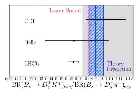
Figure 2: Compilation of measurements of the ratio of branching ratios as given in (5) and comparison with the lower bound in (26). The theoretical prediction indicated by the vertical band corresponds to (63) as given in Section 5.

In the next section, we shall use data from the $B$ factories to obtain a sharper picture of the hadronic parameters, including the CP-conserving strong phases $\delta_{s}$.

3 Hadronic Parameters from $B_{d}\to D_{(s)}^{(*)\pm}\pi^{\mp}$ Data

Using the $U$-spin flavour symmetry of strong interactions, the hadronic parameters $x_{s}$ and $\delta_{s}$ of the $B_{s}\to D_{s}^{(*)\pm}K^{\mp}$ channels can be related to their counterparts $x_{d}$ and $\delta_{d}$ of the $B_{d}\to D^{(*)\pm}\pi^{\mp}$ decays as follows [2]:

$$x_{s}=-\frac{x_{d}}{\epsilon},\quad\delta_{s}=\delta_{d}.$$ (27)

These relations assume exact $U$-spin symmetry; the impact of possible corrections will be addressed below.

The BaBar [26] and Belle [27] collaborations have performed measurements which allow us to constrain the hadronic parameters $|x_{d}|$ and $\delta_{s}$. For the $B_{d}\to D^{\pm}\pi^{\mp}$ system the following constraints have been extracted from studies of CP-violating effects [3]:

$$a^{D\pi} \equiv -2|x_{d}|\sin(\phi_{d}+\gamma)\cos(\delta_{d})=-0.03\pm 0.017,$$ (28)

$$c_{\rm lep}^{D\pi} \equiv -2|x_{d}|\cos(\phi_{d}+\gamma)\sin(\delta_{d})=-0.022\pm 0.021.$$ (29)

A corresponding analysis of the $B_{d}\to D^{*\pm}\pi^{\mp}$ decays (for which $L=1$) yields [3]

$$a^{D^{*}\pi} \equiv 2|x^{V}_{d}|\sin(\phi_{d}+\gamma)\cos(\delta^{V}_{d})=-0.039\pm 0.010,$$ (30)

$$c_{\rm lep}^{D^{*}\pi} \equiv 2|x^{V}_{d}|\cos(\phi_{d}+\gamma)\sin(\delta^{V}_{d})=-0.010\pm 0.013,$$ (31)

where we have used the label $V$ to distinguish the vector $D^{*}$ system. In order to convert these experimental results into $|x_{d}|$ and $\delta_{d}$, we assume the value for $\gamma$ in (3) with the $B^{0}_{d}$–$\bar{B}^{0}_{d}$ mixing phase $\phi_{d}\equiv 2\beta=(42.8\pm 1.6)^{\circ}$ [3], which yields $\phi_{d}+\gamma=(111\pm 7)^{\circ}$.

Let us first extract $|x_{d}|$ by determining the doubly Cabibbo-suppressed branching ratio ${\rm BR}(\bar{B}_{d}^{0}\to D^{-}\pi^{+})$ from ${\rm BR}(\bar{B}_{d}^{0}\to D_{s}^{-}\pi^{+})$ with the help of the $SU(3)$ flavour symmetry [28]. Using the notation of Ref. [23], we write

$${\rm BR}(\bar{B}^{0}_{d}\to D^{-}\pi^{+})=\left(\frac{\epsilon}{{\cal C}^{\prime}}\right){\rm BR}(\bar{B}^{0}_{d}\to D_{s}^{-}\pi^{+}),$$ (32)

where

$${\cal C}^{\prime}\equiv\frac{\Phi_{D_{s}\pi}}{\Phi_{D\pi}}{\cal N}^{\prime}_{F}{\cal N}^{\prime}_{a}{\cal N}^{\prime}_{E}.$$ (33)

In analogy to (20), the $\Phi$ are are phase-space factors, while

$${\cal N}^{\prime}_{F}\equiv\left[\frac{f_{D_{s}}}{f_{D}}\,\frac{F_{1}^{\bar{B}^{0}_{d}\pi^{+}}(m^{2}_{D_{s}})}{F_{1}^{\bar{B}^{0}_{d}\pi^{+}}(m^{2}_{D})}\right]^{2}$$ (34)

and

$${\cal N}^{\prime}_{a}\equiv\left|\frac{a_{1}(D_{s}^{+}\pi^{-})}{a_{1}(D^{+}\pi^{-})}\right|^{2}$$ (35)

describe factorizable and non-factorizable $SU(3)$-breaking effects, respectively. The ${\cal N}^{\prime}_{E}$ factor takes into account that $\bar{B}^{0}_{d}\to D^{-}\pi^{+}$ has a contribution from an exchange topology, which does not have a counterpart in the $\bar{B}^{0}_{d}\to D_{s}^{-}\pi^{+}$ channel:

$${\cal N}^{\prime}_{E}\equiv\left|\frac{T_{D^{-}\pi^{+}}}{T_{D^{-}\pi^{+}}+E_{D^{-}\pi^{+}}}\right|^{2}.$$ (36)

We then obtain the following additional constraint for $x_{d}$:

$$|x_{d}|=\sqrt{\left(\frac{\epsilon}{{\cal C}^{\prime}}\right)\left[\frac{{\rm BR}(\bar{B}^{0}_{d}\to D_{s}^{-}\pi^{+})}{{\rm BR}(\bar{B}^{0}_{d}\to D^{+}\pi^{-})}\right]}.$$ (37)

For the numerical analysis, we use the ratio of decay constants $f_{D_{s}}/f_{D}=1.25\pm 0.06$ [24] and the form-factor ratio $F_{1}^{\bar{B}^{0}_{d}\pi^{+}}(m^{2}_{D})/F_{1}^{\bar{B}^{0}_{d}\pi^{+}}(m^{2}_{D_{s}})=0.9771\pm 0.0009$, where we have applied the evolution equation for the $\bar{B}^{0}_{d}\to\pi^{+}$ form factor given in Ref. [29]. For the decays entering (32), factorization is not expected to work well. Indeed, following the approach discussed in Ref. [23], we extract $|a_{1}(D_{s}^{+}\pi^{-})|=0.68\pm 0.12$ from the experimental data, while factorization would correspond to a value around one. Unfortunately, an analogous factorization test for $\bar{B}_{d}^{0}\to D^{-}\pi^{+}$ cannot be performed. We allow for 20% $SU(3)$-breaking effects for the non-factorizable contributions, i.e. for the deviation of $|a_{1}|$ from one, leading to ${\cal N}^{\prime}_{a}=1.0\pm 0.2$.

In order to estimate the importance of the exchange contribution, we apply the $SU(3)$ flavour symmetry and use experimental information on $\mbox{BR}(\bar{B}^{0}_{d}\to D_{s}^{+}K^{-})=(2.2\pm 0.5)\times 10^{-5}$ [24], which receives only contributions from exchange topologies. Comparing it to the contribution from tree topologies, which we fix again through ${\rm BR}(\bar{B}_{d}^{0}\to D_{s}^{-}\pi^{+})=\left(2.16\pm 0.26\right)\times 10^{-5}$ [30], we obtain:

$$\left|\frac{E_{D^{-}\pi^{+}}}{T_{D^{-}\pi^{+}}}\right|\sim\frac{f_{\pi}}{f_{K}}\left|\frac{V_{ub}}{V_{cb}}\right|\sqrt{\frac{\mbox{BR}(\bar{B}^{0}_{d}\to D_{s}^{+}K^{-})}{\mbox{BR}(\bar{B}^{0}_{d}\to D_{s}^{-}\pi^{+})}}\sim 0.1.$$ (38)

Consequently, we estimate ${\cal N}^{\prime}_{E}\sim 1.0\pm 0.2$. In comparison with the value of ${\cal N}_{E}\sim 0.97\pm 0.08$ given after (23), this range is larger. Although the exchange topologies entering both quantities are estimated to have similar absolute size, the analysis performed in Ref. [23] indicates a large angle between the $E$ and $T$ amplitudes, which reduces the impact of $E$ on the amplitude ratio in ${\cal N}_{E}$.

Using finally also the experimental branching ratio ${\rm BR}(\bar{B}_{d}^{0}\to D^{+}\pi^{-})=\left(2.68\pm 0.13\right)\times 10^{-3}$ [24], the relation in (37) gives

$$|x_{d}|=0.0163\pm\left.0.0011\right|_{\rm BR}\left.\pm 0.0026\right|_{SU(3)}=0.0163\pm 0.0028.$$ (39)

This value is consistent with the results for $x_{d}$ given in Ref. [30]. Combining (39) with (28) and (29) allows, in principle, the determination of $\phi_{d}+\gamma$ and $\delta_{d}$ up to discrete ambiguities. Unfortunately, a corresponding numerical fit leaves these parameters still largely unconstrained.

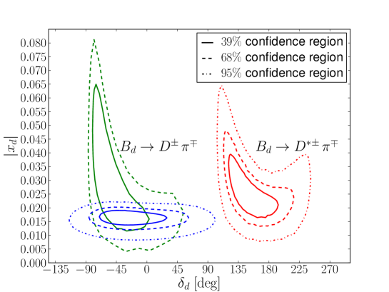
Figure 3: The confidence level contours for the $\chi^{2}$ fit of the hadronic parameters $|x_{d}|$ and $\delta_{d}$ as discussed in the text, illustrating also the impact of the $|x_{d}|$ constraint in (39).

We proceed to extract the parameters $|x_{d}|,\delta_{d}$ and $|x_{d}^{V}|,\delta_{d}^{V}$ from the constraints in (28)–(31) using a $\chi^{2}$ fit. For the former parameter set we also include the constraint in (39). The fit gives the following results:

$$|x_{d}| =0.0166^{+0.0025}_{-0.0029}, \delta_{d} =\left(-35^{+65}_{-35}\right)^{\circ},$$ (40)

$$|x^{V}_{d}| =0.025^{+0.014}_{-0.008}, \delta^{V}_{d} =\left(146^{+48}_{-25}\right)^{\circ},$$ (41)

where the errors give the $68\%$ confidence level for each parameter. The $\chi^{2}/n_{\rm dof}$ is 0.53 and 0.00 for the non-vector and vector decays, respectively. In Fig. 3, we show the corresponding 39%, 68% and 95% confidence level regions in the $\delta_{d}$–$|x_{d}|$ plane. Note that the constraint in (39) considerably reduces the uncertainty of the $|x_{d}|$ parameter for the non-vector decay.

Using (27), we hereby find

$$x_{s} =0.311^{+0.046}_{-0.053}\big{|}_{\rm input}\pm 0.06\big{|}_{SU(3)}, \delta_{s} =\left[-35^{+69}_{-40}\big{|}_{\rm input}\pm 20\big{|}_{SU(3)}\right]^{\circ},$$ (42)

$$x^{V}_{s} =0.47^{+0.26}_{-0.15}\big{|}_{\rm input}\pm 0.09\big{|}_{SU(3)}, \delta^{V}_{s} =\left[146^{+48}_{-25}\big{|}_{\rm input}\pm 20\big{|}_{SU(3)}\right]^{\circ},$$ (43)

where we allow for $SU(3)$-breaking effects of 20% for the $x^{(V)}_{s}$ parameters and $\pm 20^{\circ}$ for the strong phases. In later applications of these results, the uncertainties associated with the $x^{(V)}_{d}$, $\delta^{(V)}_{d}$ parameters and the $SU(3)$-breaking effects will be combined in quadrature.

Before using the hadronic parameters given above to predict the observables of the $B_{s}\to D_{s}^{(*)\pm}K^{\mp}$ decays in Section 5, which serve as input for an experimental study, let us first discuss the extraction of $\phi_{s}+\gamma$ from these channels, with a special emphasis on multiple discrete ambiguities and their resolution.

4 Extraction of $\phi_{s}+\gamma$ and Discrete Ambiguities

For the extraction of $\phi_{s}+\gamma$ from the $B_{s}\to D_{s}^{(*)\pm}K^{\mp}$ system, it is necessary to measure the following CP asymmetries from time-dependent, tagged analyses:

$$a_{\rm CP}(B_{s}(t)\to D_{s}^{(*)+}K^{-}) \equiv\frac{\Gamma(B^{0}_{s}(t)\to D_{s}^{(*)+}K^{-})-\Gamma(\bar{B}^{0}_{s}(t)\to D_{s}^{(*)+}K^{-})}{\Gamma(B^{0}_{s}(t)\to D_{s}^{(*)+}K^{-})+\Gamma(\bar{B}^{0}_{s}(t)\to D_{s}^{(*)+}K^{-})}$$

$$=\frac{{C}\,\cos(\Delta M_{s}\,t)+{S}\,\sin(\Delta M_{s}\,t)}{\cosh(y_{s}\,t/\tau_{B_{s}})+{\cal A}_{\Delta\Gamma}\,\sinh(y_{s}\,t/\tau_{B_{s}})};$$ (44)

an analogous expression holds for the CP-conjugate $D_{s}^{(*)-}K^{+}$ final states, where $C$, $S$ and ${\cal A}_{\Delta\Gamma}$ are simply replaced by $\overline{C}$, $\overline{S}$ and $\overline{{\cal A}}_{\Delta\Gamma}$, respectively. The observables take the following form [2]:

$$C=-\left[\frac{1-x_{s}^{2}}{1+x_{s}^{2}}\right],\quad\overline{C}=+\left[\frac{1-x_{s}^{2}}{1+x_{s}^{2}}\right]$$ (45)

$$S=(-1)^{L}\frac{2\,x_{s}}{1+x_{s}^{2}}\sin(\phi_{s}+\gamma+\delta_{s}),\quad\overline{S}=(-1)^{L}\frac{2\,x_{s}}{1+x_{s}^{2}}\sin(\phi_{s}+\gamma-\delta_{s}),$$ (46)

which complement the expressions for ${\cal A}_{\Delta\Gamma}$ and $\overline{{\cal A}}_{\Delta\Gamma}$ in (8).

For the following discussion, it is convenient to introduce the observable combinations

$$\langle C\rangle_{\pm}\equiv\frac{\overline{C}\pm C}{2},\quad\langle S\rangle_{\pm}\equiv\frac{\overline{S}\pm S}{2},$$ (47)

as well as

$$s_{+}\equiv(-1)^{L}\left[\frac{1+x_{s}^{2}}{2\,x_{s}}\right]\langle S\rangle_{+}=+\cos\delta_{s}\sin(\phi_{s}+\gamma)$$ (48)

$$s_{-}\equiv(-1)^{L}\left[\frac{1+x_{s}^{2}}{2\,x_{s}}\right]\langle S\rangle_{-}=-\sin\delta_{s}\cos(\phi_{s}+\gamma),$$ (49)

where

$$x_{s}=\sqrt{\frac{1-\langle C\rangle_{-}}{1+\langle C\rangle_{-}}},\quad\mbox{yielding}\quad\frac{1+x_{s}^{2}}{2\,x_{s}}=\frac{1}{\sqrt{1-\langle C\rangle_{-}^{2}}}.$$ (50)

Finally, we obtain

$$\sin(\phi_{s}+\gamma)=\pm\sqrt{\frac{1}{2}\left[(1+s_{+}^{2}-s_{-}^{2})\pm\sqrt{(1+s_{+}^{2}-s_{-}^{2})^{2}-4s_{+}^{2}}\right]},$$ (51)

which results in an eightfold solution for $\phi_{s}+\gamma$ [1, 2].

As was pointed out in Ref. [2], and later also in Refs. [31, 32, 33], the observable combinations

$$\langle{\cal A}_{\Delta\Gamma}\rangle_{+}\equiv\frac{\overline{\cal A}_{\Delta\Gamma}+{\cal A}_{\Delta\Gamma}}{2}=-(-1)^{L}\left[\frac{2\,x_{s}}{1+x_{s}^{2}}\right]\cos\delta_{s}\cos(\phi_{s}+\gamma)$$ (52)

$$\langle{\cal A}_{\Delta\Gamma}\rangle_{-}\equiv\frac{\overline{\cal A}_{\Delta\Gamma}-{\cal A}_{\Delta\Gamma}}{2}=-(-1)^{L}\left[\frac{2\,x_{s}}{1+x_{s}^{2}}\right]\sin\delta_{s}\sin(\phi_{s}+\gamma)$$ (53)

can be combined with the mixing-induced CP asymmetries $\langle S\rangle_{\pm}$ to derive the relation

$$\tan(\phi_{s}+\gamma)=-\frac{\langle S\rangle_{+}}{\langle{\cal A}_{\Delta\Gamma}\rangle_{+}}=\frac{\langle{\cal A}_{\Delta\Gamma}\rangle_{-}}{\langle S\rangle_{-}},$$ (54)

which allows the extraction of $\phi_{s}+\gamma$ up to a twofold ambiguity; moreover, we have

$$|\tan(\phi_{s}+\gamma)|=\sqrt{\frac{\langle{\cal A}_{\Delta\Gamma}\rangle^{2}_{-}+\langle S\rangle^{2}_{+}}{\langle S\rangle^{2}_{-}+{\langle{\cal A}_{\Delta\Gamma}\rangle^{2}_{+}}}}=\sqrt{\frac{\langle{\cal A}_{\Delta\Gamma}\rangle^{2}_{-}-\langle S\rangle^{2}_{+}}{\langle S\rangle^{2}_{-}-{\langle{\cal A}_{\Delta\Gamma}\rangle^{2}_{+}}}}.$$ (55)

The final ambiguity can be resolved from factorization arguments, where we expect

$$\cos\delta_{s}>0,\quad\cos\delta_{s}^{V}<0,$$ (56)

a pattern that agrees well with the results of the $U$-spin analysis presented in Section 3, where the results for the strong phases in (42) and (43) give

$$\cos\delta_{s}=0.82^{+0.18}_{-0.56},\quad\cos\delta_{s}^{V}=-0.83^{+0.43}_{-0.17}.$$ (57)

Combining this with (48), the sign of $\sin(\phi_{s}+\gamma)$ can then be determined. Thus, under reasonable assumptions, the extraction of $\phi_{s}+\gamma$ is unambiguous [2]. A discussion of the resolution of these discrete ambiguities was also given in Ref. [16].

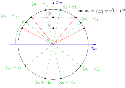
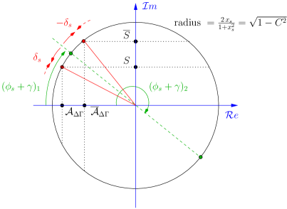
Figure 4: Illustration of the complex numbers $({\cal A}_{\Delta\Gamma}+iS)$ and $(\overline{\cal A}_{\Delta\Gamma}+i\,\overline{S})$ with lengths $\sqrt{1-C^{2}}$ in the complex plane. Left panel: illustration of the extraction of $\phi_{s}+\gamma$ without the use of untagged information and the associated eightfold discrete ambiguity (see (51)). Right panel: illustration of the reduction of the discrete ambiguity to a twofold one through the untagged observables ${\cal A}_{\Delta\Gamma}$ and $\overline{\cal A}_{\Delta\Gamma}$ (see (54)).

It is instructive to illustrate these features, which can be hidden in a global experimental fit (see Section 5). As the observables satisfy

$${C}^{2}+S^{2}+{\cal A}^{2}_{\Delta\Gamma}=1=\overline{C}^{2}+\overline{S}^{2}+\overline{\cal A}_{\Delta\Gamma}^{2}$$ (58)

and are hence not independent, only two of the three observables for each of the final states of the $B_{s}\to D_{s}^{(*)\pm}K^{\mp}$ system are needed for the determination of $\phi_{s}+\gamma$. We introduce the complex numbers

$${\cal A}_{\Delta\Gamma}+i\,{S} =-(-1)^{L}\sqrt{1-C^{2}}\,e^{-i(\phi_{s}+\gamma+\delta_{s})}$$ (59)

$$\overline{\cal A}_{\Delta\Gamma}+i\,\overline{S} =-(-1)^{L}\sqrt{1-\overline{C}^{2}}\,e^{-i(\phi_{s}+\gamma-\delta_{s})},$$ (60)

which, as $C=-\overline{C}$ (see (45)), have the same absolute value and thus span the same circle in the complex plane. The weak phase $\phi_{s}+\gamma$ corresponds to the polar angle of a complex number that lies exactly between (59) and (60), with an equal angular distance of $\delta_{s}$ to both.

Let us first have a look at the strategy, which does not use the information provided by the untagged ${\cal A}_{\Delta\Gamma}$, $\overline{\cal A}_{\Delta\Gamma}$ observables. The $C$ and $\overline{C}$ then fix a circle in the complex plane, while the mixing-induced CP asymmetries $S$, $\overline{S}$ fix the component in the imaginary direction. As illustrated in the left panel of Fig. 4, this results in an eightfold discrete ambiguity for $\phi_{s}+\gamma$. On the contrary, as shown in the right panel of Fig. 4, if the mixing-induced CP asymmetries are measured together with the untagged observables, the discrete ambiguity is reduced to a twofold one, which can be fully resolved as discussed above. Consequently, the optimal observable sets for the extraction of $\phi_{s}+\gamma$ are $S$, $\overline{S}$ and ${\cal A}_{\Delta\Gamma}$, $\overline{\cal A}_{\Delta\Gamma}$.

Another important advantage of these observables is not only that they depend linearly on $x_{s}$ – in contrast to $C$, $\overline{C}$ and the determination of this parameter through (25) – but that $x_{s}$ drops out in (54) and (55). Interestingly, as we will see in the next section, both observable sets can be accessed with similar precision at LHCb: the extraction of the untagged ${\cal A}_{\Delta\Gamma}$, $\overline{\cal A}_{\Delta\Gamma}$ observables relies on the $B_{s}$ decay width parameter (4), while the measurement of the $S$, $\overline{S}$ observables requires the tagging of the flavour of the initially produced $B^{0}_{s}$ or $\bar{B}_{s}^{0}$ mesons.

5 Experimental Prospects

The hadronic parameters determined in Section 3, with the phases in (1) and (3), allow us to make predictions of the observables of the $B_{s}\to D_{s}^{\pm}K^{\mp}$ decays:

$$\tau_{\rm eff} =0.971^{+0.053}_{-0.012}\ \tau_{B_{s}}, {\cal A}_{\Delta\Gamma} =-0.49^{+0.58}_{-0.13}, C =-0.824^{+0.086}_{-0.077}, S =0.29^{+0.30}_{-0.40},$$

$$\bar{\tau}_{\rm eff} =1.025^{+0.030}_{-0.054}\ \tau_{B_{s}}, \overline{\cal A}_{\Delta\Gamma} =0.11^{+0.34}_{-0.59}, \overline{C} =0.824^{+0.077}_{-0.086}, \overline{S} =0.55^{+0.11}_{-0.28}.$$ (61)

In analogy, for the $B_{s}\to D_{s}^{*\pm}K^{\mp}$ decays we obtain

$$\tau^{V}_{\rm eff} =0.954^{+0.057}_{-0.021}\ \tau_{B_{s}}, {\cal A}_{\Delta\Gamma}^{V} =-0.66^{+0.60}_{-0.21}, C^{V} =-0.64^{+0.36}_{-0.20}, S^{V} =0.40^{+0.39}_{-0.44},$$

$$\bar{\tau}^{V}_{\rm eff} =1.027^{+0.034}_{-0.060}\ \tau_{B_{s}}, \overline{\cal A}_{\Delta\Gamma}^{V} =0.13^{+0.40}_{-0.66}, \overline{C}^{V} =0.64^{+0.20}_{-0.36}, \overline{S}^{V} =0.76^{+0.19}_{-0.30}.$$ (62)

Furthermore, our predictions for the branching ratio observables (5) and (13) are

$$\left.\frac{\text{BR}(B_{s}\rightarrow D_{s}^{\pm}K^{\mp})_{\rm exp}}{\text{BR}(B_{s}\rightarrow D_{s}^{\pm}\pi^{\mp})_{\rm exp}}\right|_{SU(3)} =0.0864^{+0.0087}_{-0.0072},$$ (63)

$$\left.\frac{{\rm BR}(B_{s}\to D_{s}^{+}K^{-})_{\rm exp}-{\rm BR}(B_{s}\to D_{s}^{-}K^{+})_{\rm exp}}{{\rm BR}(B_{s}\to D_{s}^{+}K^{-})_{\rm exp}+{\rm BR}(B_{s}\to D_{s}^{-}K^{+})_{\rm exp}}\right|_{SU(3)} =-0.027^{+0.052}_{-0.019},$$ (64)

respectively. The prediction in (63) is compared to the current experimental results in Fig. 2. Similarly, we predict for the vector decays:

$$\left.\frac{\text{BR}(B_{s}\rightarrow D_{s}^{*\pm}K^{\mp})_{\rm exp}}{\text{BR}(B_{s}\rightarrow D_{s}^{*\pm}\pi^{\mp})_{\rm exp}}\right|_{SU(3)} =0.099^{+0.030}_{-0.036},$$ (65)

$$\left.\frac{{\rm BR}(B_{s}\to D_{s}^{*+}K^{-})_{\rm exp}-{\rm BR}(B_{s}\to D_{s}^{*-}K^{+})_{\rm exp}}{{\rm BR}(B_{s}\to D_{s}^{*+}K^{-})_{\rm exp}+{\rm BR}(B_{s}\to D_{s}^{*-}K^{+})_{\rm exp}}\right|_{SU(3)} =-0.035^{+0.056}_{-0.024}.$$ (66)

To estimate the experimental sensitivity for the observables, a simple Monte Carlo simulation has been performed, using as theoretical input the central values $x_{s}=0.311$, $\delta_{s}=-35^{\circ}$ (see (42)), $\Delta m_{s}=17.72\,\mathrm{ps}^{-1}$ [34], $y_{s}=0.088$ (see (4)) and $\gamma+\phi_{s}=65.5^{\circ}$ (see (1) and (3)). A global fit to the decay distributions then simultaneously determines the observables given in (61).

Table 1: Statistical uncertainties of $B_{s}^{0}\rightarrow D_{s}^{\pm}K^{\mp}$ CP observables for various data samples as determined from our toy study. The difference in sensitivity of $\langle\mathcal{A}_{\Delta\Gamma}\rangle_{+}$, $\langle\mathcal{A}_{\Delta\Gamma}\rangle_{-}$ is due to a correlation between $\mathcal{A}_{\Delta\Gamma}$ and $\overline{\mathcal{A}}_{\Delta\Gamma}$ of 0.5 observed in our toy simulations.

Scenario	$\sigma(C\>,\>\overline{C})$	$\sigma(S\>,\>\overline{S})$	$\sigma(\mathcal{A}_{\Delta\Gamma}\>,\overline{\mathcal{A}}_{\Delta\Gamma})$	$\sigma(\langle S\rangle_{\pm})$	$\sigma(\langle\mathcal{A}_{\Delta\Gamma}\rangle_{+})$	$\sigma(\langle\mathcal{A}_{\Delta\Gamma}\rangle_{-})$
LHCb end 2012	$\pm 0.176$	$\pm 0.252$	$\pm 0.210$	$\pm 0.173$	$\pm 0.194$	$\pm 0.113$
LHCb 2018	$\pm 0.077$	$\pm 0.110$	$\pm 0.092$	$\pm 0.076$	$\pm 0.085$	$\pm 0.049$
LHCb Upgrade	$\pm 0.032$	$\pm 0.046$	$\pm 0.038$	$\pm 0.032$	$\pm 0.035$	$\pm 0.020$

Table 2: Experimental uncertainties on the weak phase $\phi_{s}+\gamma$, strong phase $\delta_{s}$ and hadronic parameter $x_{s}$ for various data samples as determined from our toy simulations. Results for the method, which excludes the untagged observables, are also shown. The errors correspond to the central values $\phi_{s}+\gamma=65.5^{\circ}$, $\delta_{s}=-35^{\circ}$ and $x_{s}=0.31$.

	With $\mathcal{A}_{\Delta\Gamma}$ and $\overline{\mathcal{A}}_{\Delta\Gamma}$			Only tagged information
Scenario	$\phi_{s}+\gamma$	$\delta_{s}$	$x_{s}$	$\phi_{s}+\gamma$	$\delta_{s}$	$x_{s}$
LHCb end 2012	$[\pm 17]^{\circ}$	$[\pm 17]^{\circ}$	$\pm 0.080$	-	-	$\pm 0.11\phantom{0}$
LHCb 2018	$[\pm 7.3]^{\circ}$	$[\pm 7.3]^{\circ}$	$\pm 0.035$	$[^{+16}_{-26}]^{\circ}$	$[^{+26}_{-16}]^{\circ}$	$\pm 0.048$
LHCb Upgrade	$[\pm 3.0]^{\circ}$	$[\pm 3.0]^{\circ}$	$\pm 0.015$	$[^{+8.8}_{-19}]^{\circ}$	$[^{+19}_{-8.8}]^{\circ}$	$\pm 0.021$

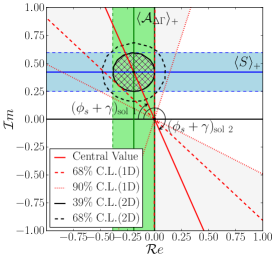
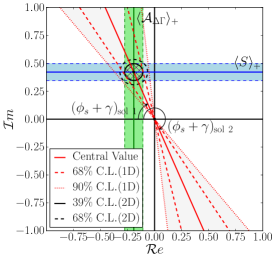
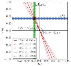
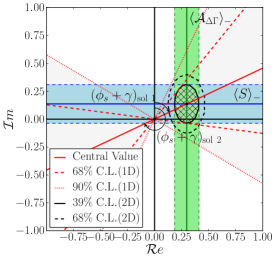
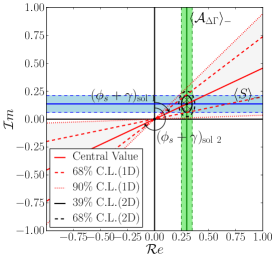
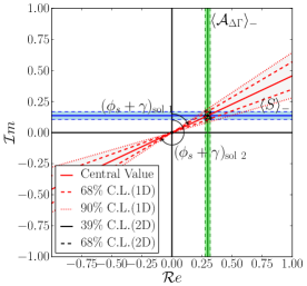
Figure 5: Illustration of the determination of $\phi_{s}+\gamma$ from the separate observable combinations $\langle{\cal A}_{\Delta\Gamma}\rangle_{+}$ and $\langle S\rangle_{+}$ (top row) and $\langle{\cal A}_{\Delta\Gamma}\rangle_{-}$ and $\langle S\rangle_{-}$ (bottom row); see (67) and (68). The increasing experimental sensitivity of the panels from left to right corresponds to expectations of the LHCb experiment by the end of 2012, before the upgrade and after the upgrade, respectively.

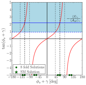
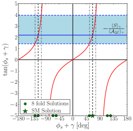
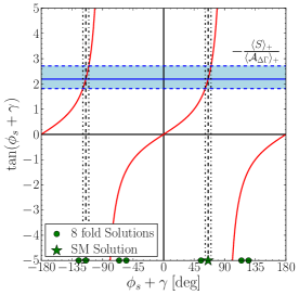
Figure 6: Illustration of the determination of $\phi_{s}+\gamma$ from $\langle{\cal A}_{\Delta\Gamma}\rangle_{+}$ and $\langle S\rangle_{+}$ by means of (54). We also show the eightfold solution resulting from the method (51) that does not use untagged information, as discussed in the text. The increasing experimental sensitivity of the panels from left to right corresponds to expectations of the LHCb experiment by the end of 2012, before the upgrade and after the upgrade, respectively.

Experimental data sets are simulated assuming approximate detector performance, as discussed in Ref. [34] by the LHCb collaboration, corresponding to a decay-time resolution of 50 fs, a flavour tagging efficiency of 38%, and a wrong-tag probability of 34%. The sensitivity is estimated for data sets that would correspond to about 1100 events per fb^-1 of collected integrated luminosity [14], selecting only $B_{s}$ candidates with a lifetime of $t>0.5$ ps. Systematic effects, such as the presence of background events, are ignored in this study.

In the toy simulation, the observables listed in (61) are determined from a fit to the decay distributions from 3500 simulated $B_{s}\rightarrow D_{s}^{\pm}K^{\mp}$ events corresponding to the approximate data sample that can be collected by the LHCb experiment by the end of 2012. The fit is repeated for 2000 different data sets, resulting in an estimate for the sensitivity for the observables, which is comparable to the accuracy of the prediction itself. In Table 1, the statistical uncertainties for the observables are listed for data samples corresponding to the expected integrated luminosity of the LHCb experiment at the end of 2012, before the upgrade, and after the upgrade. In our toy simulations an average correlation of 0.5 was observed between the $\mathcal{A}_{\Delta\Gamma}$ and $\overline{\mathcal{A}}_{\Delta\Gamma}$ observables, which is taken into account in the fits below; the correlations between the other CP observables is found to be negligible.

As a final step, these estimated experimental uncertainties for the observables $\mathcal{A}_{\Delta\Gamma}$, $S$, $C$ and their CP conjugates can be translated into a determination for $\gamma$. Using only $S$, $\overline{S}$ and $C$, $\overline{C}$ following the approach without using untagged information, as described by (51), the experimental sensitivity is not sufficient to determine $\gamma$ for a data sample of about 3500 events, which can be collected by the end of 2012. A factor five increase in data size, corresponding to the end of the current LHCb experiment, would result in a sensitivity of $\gamma+\phi_{s}=(65.6^{+17}_{-26})^{\circ}$ if the solution around the input value for $\gamma$ is selected.

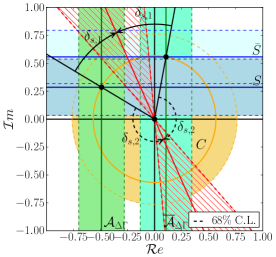
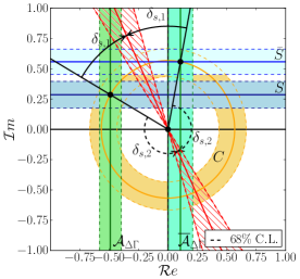
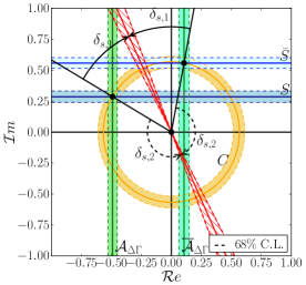
Figure 7: Illustration of the determination of $\phi_{s}+\gamma$ from a simultaneous fit to ${\cal A}_{\Delta\Gamma}$, ${\cal S}$, $C$ and their CP conjugates in the complex plane (see also Fig. 4). The 68% confidence levels for $\phi_{s}+\gamma$ and the CP observables are indicated by the hatched and shaded regions, respectively. The two solutions shown for $\phi_{s}+\gamma$ and $\delta_{s}$ correspond to the remaining twofold discrete ambiguity discussed in the text. The increasing experimental sensitivity of the panels from left to right corresponds to expectations of the LHCb experiment by the end of 2012, before the upgrade and after the upgrade, respectively.

If instead the observable pairs

$$\langle{\cal A}_{\Delta\Gamma}\rangle_{+}+i\langle S\rangle_{+}=-(-1)^{L}\sqrt{1-\langle C\rangle^{2}_{-}}\cos\delta_{s}\,e^{-i(\phi_{s}+\gamma)}$$ (67)

and

$$\langle{\cal A}_{\Delta\Gamma}\rangle_{-}+i\langle S\rangle_{-}=-(-1)^{L}\sqrt{1-\langle C\rangle^{2}_{-}}\sin\delta_{s}\,e^{i(\pi/2-(\phi_{s}+\gamma))}$$ (68)

are used separately, the 2012 data sample corresponds to experimental sensitivities for $\gamma+\phi_{s}$ of $\pm 24^{\circ}$ and $\pm 29^{\circ}$, respectively; see the left panel of Fig. 5. In Fig. 6, we illustrate the extraction of $\gamma+\phi_{s}$ from $\langle S\rangle_{+}$ and $\langle{\cal A}_{\Delta\Gamma}\rangle_{+}$ by means of the first relation in (54). Finally, combining all the observables, i.e. ${\cal A}_{\Delta\Gamma}$, ${\cal S}$ and $C$ with their CP conjugates, improves the sensitivity to $\pm 17^{\circ}$, as illustrated in the left panel of Fig. 7.

With increasing data samples, shown in the middle and right panels of Figs. 5–7, the precision on the measurement of $\gamma+\phi_{s}$ is expected to increase to about $\pm 7^{\circ}(3^{\circ})$ using 18k(130k) $B_{s}\rightarrow D_{s}^{\pm}K^{\mp}$ events, which could finally be collected by the current (upgraded) LHCb experiment, assuming unchanged trigger and tagging performance. The sensitivity quoted here is different, but compatible with the projected sensitivity quoted by the LHCb collaboration [35], where more sophisticated estimates are made for the trigger performance in the coming running periods. The different experimental errors for the determination of $\phi_{s}+\gamma$, $\delta_{s}$ and $x_{s}$ from the $B_{s}\rightarrow D_{s}^{\pm}K^{\mp}$ decays are collected in Table 2.

The magnitude of $\mathcal{A}_{\Delta\Gamma}+iS$ can be further constrained through the $SU(3)$ flavour symmetry, i.e. through (25) or by means of (27) with (37). However, we find that this input, which would introduce the $SU(3)$ flavour symmetry into a theoretically clean strategy, does not significantly improve the precision for $\gamma+\phi_{s}$.

On the other hand, if also decays of the type $B_{s}\rightarrow D_{s}^{*\pm}K^{\mp}$ can be reconstructed, the precision could be further enhanced in a theoretically clean way. These channels require the reconstruction of a radiative photon in the decay $D_{s}^{*\pm}\rightarrow D_{s}^{\pm}\gamma$ and as such are experimentally more challenging. In Ref. [36], a gain in statistics of 28% is deemed possible, leading to an improvement of 13% on the determination of $\phi_{s}+\gamma$.

6 Conclusions

The decays $B_{s}\to D_{s}^{(*)\pm}K^{\mp}$ offer an interesting playground for the LHCb experiment in this decade. We have performed a detailed analysis of the observables of these channels, addressing in particular the impact of the sizable $B_{s}$ decay width difference $\Delta\Gamma_{s}$, which has recently been established. This quantity leads to a subtle difference between the experimental and theoretical branching ratios of the $B_{s}\to D_{s}^{(*)\pm}K^{\mp}$ decays, which can be resolved experimentally through time information on the corresponding untagged data samples, such as measurements of the effective decay lifetimes. We derived a lower bound for the ratio of the experimental $B_{s}\to D_{s}^{\pm}K^{\mp}$ and $B_{s}\to D_{s}^{\pm}\pi^{\mp}$ branching ratios given in (5), and observe that the central value for the LHCb result is too small by about two standard deviations.

The width difference $\Delta\Gamma_{s}$ offers the untagged observables ${\cal A}_{\Delta\Gamma}$ and $\overline{\cal A}_{\Delta\Gamma}$ for the final states $D_{s}^{(*)+}K^{-}$ and $D_{s}^{(*)-}K^{+}$, respectively, which can nicely be combined with the corresponding mixing-induced CP asymmetries $S$ and $\overline{S}$ to determine $\phi_{s}+\gamma$ in an unambiguous way. We have illustrated this strategy and have obtained predictions for the $B_{s}\to D_{s}^{(*)\pm}K^{\mp}$ observables from an $SU(3)$ analysis of the $B$-factory data for $B_{d}\to D^{(*)\pm}\pi^{\mp}$, $B_{d}\to D^{\pm}_{s}\pi^{\mp}$ decays. Moreover, making experimental simulations, we have shown that the interplay between the untagged observables ${\cal A}_{\Delta\Gamma}$, $\overline{\cal A}_{\Delta\Gamma}$ and the tagged CP asymmetries $S$, $\overline{S}$ is actually the key feature for being able to measure $\phi_{s}+\gamma$ through the $B_{s}\to D_{s}^{(*)\pm}K^{\mp}$ decays at LHCb. In this sense, the favourably large value of $\Delta\Gamma_{s}$ is a present from Nature.

Acknowledgements

This work is supported by the Netherlands Organisation for Scientific Research (NWO) and the Foundation for Fundamental Research on Matter (FOM). We thank Suvayu Ali for useful discussions.

References

• [1] R. Aleksan, I. Dunietz and B. Kayser, Z. Phys. C 54 (1992) 653.
• [2] R. Fleischer, Nucl. Phys. B 671 (2003) 459 [hep-ph/0304027].
• [3] Y. Amhis et al. [Heavy Flavor Averaging Group Collaboration], arXiv:1207.1158 [hep-ex].
• [4] R. Fleischer, Phys. Lett. B 459 (1999) 306 [hep-ph/9903456]; see also I. Dunietz, FERMILAB-CONF-93-090-T.
• [5] CKMfitter Collaboration, http://ckmfitter.in2p3.fr/
• [6] UTfit Collaboration, http://www.utfit.org/UTfit/
• [7] R. Fleischer and R. Knegjens, Eur. Phys. J. C 71 (2011) 1532 [arXiv:1011.1096 [hep-ph]].
• [8] R. Aaij et al. [LHCb Collaboration], LHCb-CONF-2012-002.
• [9] R. Aaij et al. [LHCb Collaboration], Phys. Rev. Lett.  108 (2012) 241801 [arXiv:1202.4717 [hep-ex]].
• [10] A. Lenz, arXiv:1205.1444 [hep-ph].
• [11] K. de Bruyn, R. Fleischer, R. Knegjens, P. Koppenburg, M. Merk and N. Tuning, Phys. Rev. D 86 (2012) 014027 [arXiv:1204.1735 [hep-ph]].
• [12] T. Aaltonen et al. [CDF Collaboration], Phys. Rev. Lett.  103 (2009) 191802 [arXiv:0809.0080 [hep-ex]].
• [13] R. Louvot et al. [Belle Collaboration], Phys. Rev. Lett.  102 (2009) 021801 [arXiv:0809.2526 [hep-ex]].
• [14] R. Aaij et al. [LHCb Collaboration], JHEP 1206 (2012) 115 [arXiv:1204.1237 [hep-ex]].
• [15] I. Dunietz, R. Fleischer and U. Nierste, Phys. Rev. D 63 (2001) 114015 [hep-ph/0012219].
• [16] S. Nandi and U. Nierste, Phys. Rev. D 77 (2008) 054010 [arXiv:0801.0143 [hep-ph]].
• [17] D. Fakirov and B. Stech, Nucl. Phys.  B 133 (1978) 315; N. Cabibbo and L. Maiani, Phys. Lett.  B 73 (1978) 418 [Erratum-ibid.  B 76 (1978) 663].
• [18] A. J. Buras, J.-M. Gérard and R. Rückl, Nucl. Phys.  B 268 (1986) 16.
• [19] J. D. Bjorken, Nucl. Phys. Proc. Suppl.  11 (1989) 325.
• [20] M. J. Dugan and B. Grinstein, Phys. Lett.  B 255 (1991) 583.
• [21] M. Beneke, G. Buchalla, M. Neubert and C. T. Sachrajda, Nucl. Phys.  B 591 (2000) 313 [arXiv:hep-ph/0006124].
• [22] C. W. Bauer, D. Pirjol and I. W. Stewart, Phys. Rev. Lett.  87 (2001) 201806 [arXiv:hep-ph/0107002].
• [23] R. Fleischer, N. Serra and N. Tuning, Phys. Rev. D 83 (2011) 014017 [arXiv:1012.2784 [hep-ph]].
• [24] J. Beringer et al. [Particle Data Group], Phys. Rev. D 86 (2012) 010001.
• [25] I. Caprini, L. Lellouch and M. Neubert, Nucl. Phys.  B 530 (1998) 153 [arXiv:hep-ph/9712417].
• [26] B. Aubert et al. [BaBar Collaboration], Phys. Rev. D 73 (2006) 111101 [hep-ex/0602049]; Phys. Rev. D 71 (2005) 112003 [hep-ex/0504035].
• [27] F.J. Ronga et al. [Belle Collaboration], Phys. Rev. D 73 (2006) 092003 [hep-ex/0604013]; S. Bahinipati et al. [Belle Collaboration], Phys. Rev. D 84 (2011) 021101 [arXiv:1102.0888 [hep-ex]].
• [28] I. Dunietz, Phys. Lett. B 427 (1998) 179 [hep-ph/9712401].
• [29] G. Duplancic, A. Khodjamirian, T. Mannel, B. Melic and N. Offen, JHEP 0804 (2008) 014 [arXiv:0801.1796 [hep-ph]].
• [30] A. Das et al. [Belle Collaboration], Phys. Rev. D 82 (2010) 051103 [arXiv:1007.4619 [hep-ex]]; B. Aubert et al. [BaBar Collaboration], Phys. Rev. D 78, 032005 (2008) [arXiv:0803.4296 [hep-ex]].
• [31] G. Cavoto, R. Fleischer, T. Gershon, A. Soni, K. Abe, J. Albert, D. Asner and D. Atwood et al., hep-ph/0603019.
• [32] V. Gligorov and G. Wilkinson, CERN-LHCB-2008-035.
• [33] V. Gligorov [LHCb Collaboration], arXiv:1101.1201 [hep-ex].
• [34] LHCb Collaboration, R. Aaij et al., LHCb-CONF-2011-050.
• [35] I. Bediaga et al. [LHCb Collaboration], arXiv:1208.3355 [hep-ex].
• [36] J. v. Tilburg, CERN-THESIS-2005-040.