Positioning and orienting a static cylindrical radio-reflector for wide field surveys

Several projects in radioastronomy plan to use large static cylindrical reflectors with an extended lobe sampling a sector of the rotating sky. This study provides the exact mathematical expression of the transit time of a celestial object within the acceptance lobe of such a cylindrical device. The mathematical approach, based on the stereographic projection, allows one to study the optimisation of the position and orientation of the radio-reflector, and should provide exact coefficients for the spatial Fourier Transform of the radio signal along the cylinder axis.
Keywords: Instrumentation: interferometers – Cosmology: large-scale structure of Universe – dark energy – Radio lines: galaxies

1 Introduction

Several baryonic oscillation (BAO) radio projects $\!{}^{{\bf?},{\bf?},{\bf?}}$ plan to operate a series of parallel static reflectors of large parabolic cylinder shape, to map the $21cm$ HI emission line. The sky will transit over the acceptance lobe, which is defined by an angular sector of aperture $\Delta$ centered around a vertical plane (see Fig. 1).

Figure 1: The reflector and its field of view, defined as the angular sector $\Delta$ that is focalised within the antenna’s acceptance.

The projection on the sky of this angular sector can be seen on Fig. 2. In this paper, I produce the exact calculation of the transit time of a celestial object, as a function of its declination. In section 5, I use the results of the calculation to compare the performances of various radio-telescope latitudes (France, Morocco, South Africa, equator) and configurations (orientation). In particular, we show that the North-South orientation usually considered may not be the optimal one for high-z BAO studies that need large exposure times, but not necessarilly the largest possible field of view.

Another possible use of the exact expression for the transit time is the production of exact coefficients for Fourier Transform calculations along the cylinder axis.

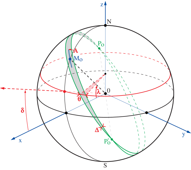
Figure 2: The celestial sphere with the projected position of the observer $M_{0}$ (latitude $\lambda$), the projected orientation of the reflector (A) and the projected portion of detectable sky (detection lobe), defined as the angular sector $\Delta$ of axis $P_{0}P^{\prime}_{0}$ (in grey), where $P_{0}$ and $P^{\prime}_{0}$ are the projections of the reflector’s axis. $\theta/2\pi$ is the fraction of the sideral day that an object of declination $\delta$ will spend within the detection lobe.

2 Notations

We will use the following notations (see Fig. 2):

• $\lambda$ is the observatory’s latitude,

• $M_{0}$ its position on Earth.

• $A$ is the azimuth of the reflector (with respect to the meridian).

• $\Delta$ is the lobe’s aperture. A celestial object can be detected only if it enters this lobe.

• $P_{0}$ and $P^{\prime}_{0}$ are the intersections of the lobe’s definition planes on the celestial sphere. $P_{0}P^{\prime}_{0}M_{0}$ define a large circle on the sphere, with $(\widehat{P_{0}OM_{0}})=(\widehat{M_{0}OP^{\prime}_{0}})=\pi/2$.

• $\delta$ is the declination of a celestial object.

The (sideral) daily exposure of an object is given by the fraction of its corresponding parallel that is included in the acceptance lobe. On Fig. 2, this exposure is given by $\theta/2\pi\times 1\,sideral\,day$. When $\lambda$, $A$ and $\Delta$ are defined, it depends only on the declination of the object. From the figure, it can be seen that the daily exposure is in general not uniform for a random choice of $\lambda$ and $A$. The objective of this paper is to systematically study the exposure as a function of the declination for any antenna configuration, and to provide an optimization tool.

3 The stereographic projection

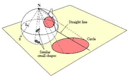
Figure 3: Stereographic projection from the North pole.

The geometrical tool used to establish the exposure versus declination function is the stereographic projection, because of the geometrical configuration includes only circles, and mainly large circles (see Fig. 3). Fig. 2 is then projected from the South pole on the equatorial plane (Fig. 4).

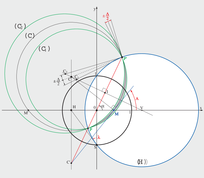
Figure 4: The stereographic projection of Fig. 2. This construction is drawn from point $S$ as follows: - $H$ is such that $(\widehat{OSH})=\lambda$. - $M$ and $M^{\prime}$, projections of $M_{0}$ and its antipod $M^{\prime}_{0}$ are the intersections of $Ox$ with the circle of radius $HS$, centered on $H$. - $C^{\prime}$ is the intersection of the vertical line containing $H$ and the line defined by $M$ (or $M^{\prime}$) and angle $A$ (or $-A$). - $C$ is the intersection of the vertical line containing $H$ and the line defined by $M$ (or $M^{\prime}$) and angle $A+\pi/2$ (or $-A+\pi/2$). - $P$ and $P^{\prime}$ are the intersections of the line $OC^{\prime}$ and the circle ${\cal C}$ of radius $CM$ centered on $C$. - $I$ is the center of $PP^{\prime}$. - The horizon circle (${\cal H}$) is centered on V, intersection of $0x$ with $IC$.

The main properties of the stereographic projection that we will use are the following:

• The projection of a circle on the sphere is a circle or a straight line on the plane.

• The projection of a large circle is a circle (or a straight line) that intercepts the equator in 2 diametrally opposite points.

• The projection of a meridian is a straight line that includes the origin.

• Angles between tangents on the sphere are invariant under the projection.

• Lengths and surfaces are not invariant under the projection, but for symmetry reasons, the scaling is constant along a given parallel. The fraction of a parallel that is included in the acceptance lobe will then be invariant under the projection.

On figure 4, the thick circle (of radius 1) is the equator, the crescent is the projection of the lobe, and the blue circle (${\cal H}$) is the projection of the horizon of $M_{0}$ (projected on $M$). We do not restrict the generality by assuming that the observatory is located in the northern hemisphere (in the reverse case, juste exchange North and South) and that $0<A<\pi/2$. The projection of the visible part of the sky is then given by the white (not shaded) area (that contains $M$ ($0<x_{M}<1$), projection of $M_{0}$). The two circles (${\cal C}_{1}$) and (${\cal C}_{2}$) are the projections of the large circles defining the lobe, that intercept each other at $P_{0}$ and $P^{\prime}_{0}$. Since $P_{0}$ and $P^{\prime}_{0}$ are on the same meridian (because they are antipodic), their projections $P$ and $P^{\prime}$ are aligned with the origin. As a consequence of the angle conservation, the projection of the large circle defining the median plane of the lobe intercepts the observer’s meridian projection (Ox axis) at angle $A$. We define $I$ as the center of $PP^{\prime}$ segment.

The horizon circle (${\cal H}$), projection of the large circle horizon of $M_{0}$, contains $P$, $P^{\prime}$, and intersects the equator at $S(0,-1)$ and $(0,1)$ with angle $\pi/2-\lambda$. Its center $V$ is aligned with $IC$ which is the median of $PP^{\prime}$ for symmetry reasons.

3.1 Useful relations

Our aim is to find the intersections of the projected lobe sides (${\cal C}_{1}$) and (${\cal C}_{2}$) with a given declination circle. In this subsection, we first determine $OI$, $IP$ and $IC$ that are needed to establish the equations of these circles.
Fig. 5 shows some important geometrical relations involving the observer’s position and its antipodic point, in the transverse view of the stereographic projection.

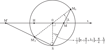
Figure 5: Vertical view of the stereographic sphere along the X axis, showing the relations between the projections $M$ and $M^{\prime}$ of two antipodic points $M_{0}$ (at latitude $\lambda$) and $M^{\prime}_{0}$. $S$ is the south pole.
$OM^{2}+OS^{2}=MS^{2}$
$OM^{\prime 2}+OS^{2}=M^{\prime}S^{2}$
$MS^{2}+M^{\prime}S^{2}=MM^{\prime 2}$
The two first relations reported in the third one give
$MM^{\prime 2}=OM^{2}+OM^{\prime 2}+2OS^{2}$
which is also equal to
$MM^{\prime 2}=(MO+OM^{\prime})^{2}=OM^{2}+OM^{\prime 2}+2.OM.OM^{\prime}$
It follows that $OM\times OM^{\prime}=OS^{2}=1$.

These relations are valid for any couple of antipodic points. The following series of relations allows to extract the most pertinent parameters of the lobe projection for subsequent calculation of the exposure time.

• $$OS=1$$ (1)

• Let $H$ be the center of $MM^{\prime}$ where $M^{\prime}$ is the projection of $M^{\prime}_{0}$, antipodic of $M_{0}$ :

  $$OH=\tan\lambda$$ (2)

  because $H$ is the center of the circle circumscribing the $MSM^{\prime}$ right triangle (Fig. 5), implying that $HS=HM$ and therefore $(\widehat{HMS})=(\widehat{MSH})=\pi/4+\lambda/2$ and $(\widehat{OSH})=(\widehat{MSH})-(\widehat{MSO})=\lambda$.

• It also follows from this that

  $$HM=HS=1/\cos\lambda$$ (3)

• As the horizon circle (${\cal H}$) intersects the equator with angle $\pi/2-\lambda$, it is tangent to $HS$; then, taking into account that $OS=1$, its center $V$ is such that

  $$OV=\cot\lambda$$ (4)

  and its radius is

  $$VS=1/\sin\lambda.$$ (5)

• Let $C$ be the center of circle (${\cal C}$) projected from the lobes’ median large circle.
  i) (${\cal C}$) includes $M$, $M^{\prime}$, $P$ and $P^{\prime}$, then its center $C$ belongs to the median of $MM^{\prime}$ (defined by $HC$ on Fig. 4).
  ii) The angle between $Ox$ (projection of the meridian) and the tangent of (${\cal C}$) at $M$ is $A$, by virtue of the angle conservation. $CM$ is then orthogonal to that tangent (see Fig. 4). It follows that :

  $$HC=\frac{HM}{\tan A}=\frac{1}{\cos\lambda\tan A}.$$ (6)

• We also define $C^{\prime}$ (bottom-left in Fig. 4) as the center of the circle projected from the large circle perpendicular to the lobe at $M_{0}$.
  i) This projected circle includes $M$ and $M^{\prime}$, then $C^{\prime}$ also belongs to the median of $MM^{\prime}$ defined by $HC$.
  ii) Since this large circle is orthogonal to the lobe, its projected circle is orthogonal to (${\cal C}$) at $M$ ; it follows that $C^{\prime}M$ is tangent to (${\cal C}$) at $M$ (see Fig. 4).
  iii) Since $P_{0}$ and $P_{0}^{\prime}$ are the poles of this large circle, for symmetry reasons, this circle intersects the $P_{0}P_{0}^{\prime}$ meridian with right angle. It follows that $PP^{\prime}$ (aligned with $O$ because $P_{0}$ and $P_{0}^{\prime}$ are on the same meridian) is perpendicular to the projected circle, and subsequently aligned with its center $C^{\prime}$ (see Fig. 4).
  It follows that :

  $$HC^{\prime}=HM.\tan A=\frac{\tan A}{\cos\lambda}.$$ (7)

• $$CC^{\prime}=HC+HC^{\prime}=\frac{1}{\cos\lambda\tan A}+\frac{\tan A}{\cos\lambda}=\frac{1}{\cos\lambda\cos A\sin A}.$$ (8)

• The angle $\alpha$, as marked on Fig. 4 will be useful for subsequent calculations.

  $$HC^{\prime}=OH\tan\alpha=\tan\lambda\tan\alpha\ (using(\ref{OH})).$$ (9)

  Combining with (7), one obtains

  $$\tan A=\sin\lambda\tan\alpha.$$ (10)

• $CC^{\prime 2}=CI^{2}+C^{\prime}I^{2}$ and $C^{\prime}I/CI=\tan\alpha=\tan A/\sin\lambda$ and (8) $=>$

  $$IC\sqrt{1+\tan^{2}A/\sin^{2}\lambda}=\frac{1}{\cos\lambda\cos A\sin A}.$$ (11)

  Then

  $$IC=\frac{\tan\lambda}{\sin A\cos A}\frac{1}{\sqrt{sin^{2}\lambda+\tan^{2}A}}$$ (12)

  and

  $$IC^{\prime}=IC\tan\alpha=IC\tan A/\sin\lambda=\frac{1}{\cos\lambda\cos^{2}A}\frac{1}{\sqrt{\sin^{2}\lambda+\tan^{2}A}}.$$ (13)

• Using relations (2) and (7) one finds:

  $$OC^{\prime}=\sqrt{OH^{2}+HC^{\prime 2}}=\sqrt{\tan^{2}\lambda+\frac{\tan^{2}A}{\cos^{2}\lambda}}=\frac{\sqrt{\sin^{2}\lambda+\tan^{2}A}}{\cos\lambda}.$$ (14)

• $OI=IC^{\prime}-OC^{\prime}$. Using (13) and (14), one obtains, after simplification:

  $$OI=\frac{\cos\lambda}{\sqrt{\sin^{2}\lambda+\tan^{2}A}}.$$ (15)

• $P$ and $P^{\prime}$ are the images of antipodic points, equivalently to $M$ and $M^{\prime}$. Using Fig. 5 the relation: $OH^{2}+OS^{2}=HS^{2}=HM^{2}$ can be transposed as $OI^{2}+1=IP^{2}$. Then

  $$IP=\sqrt{1+OI^{2}}=\frac{1}{\cos A}\frac{1}{\sqrt{\sin^{2}\lambda+\tan^{2}A}}.$$ (16)

3.2 Expression of the exposure time

The final calculations are made in the rotated frame (XoY) as shown in Fig. 6.

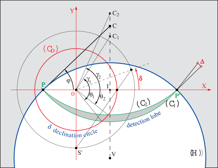
Figure 6: The projections of the detection lobe (in grey), the horizon (${\cal H}$, blue circle) and a declination circle (${\cal C}_{D}$ in red) in the rotated frame (see text). The radius of the declination circle is constructed from $S^{\prime}$ and $\delta$ similarly to the construction of $OM$ from $S$ and $\lambda$ in Fig. 5.

The parameters we will use are $OI$, $\Delta$ and $\phi$ that is given by

$$\tan\phi=IC/IP=\frac{\tan\lambda}{\sin A}$$ (17)

(from (12) and (16)). The angle $\Delta$ between the lobe’s side circles is invariant under the projection, and is shown in Fig. 6. To find the fraction of a sideral day spent by an object at declination $\delta$ within the lobe acceptance, one needs to find the intersections of the declination circle (${\cal C}_{D}$) with the images of the large circles (${\cal C}_{1}$) of center $C_{1}\,(X_{1},Y_{1})$ and (${\cal C}_{2}$) of center $C_{2}\,(X_{2},Y_{2})$. The equations of (${\cal C}_{D}$) and (${\cal C}_{1}$) are:

$$X^{2}+Y^{2} = \tan^{2}(\pi/4-\delta/2)$$ (18)

$$(X-X_{1})^{2}+(Y-Y_{1})^{2} = PC_{1}^{2}$$ (19)

$$(\ref{C1}) => X^{2}+Y^{2}-2(XX_{1}+YY_{1})+X_{1}^{2}+Y_{1}^{2}=PC_{1}^{2}$$ (20)

$$=> \tan^{2}(\pi/4-\delta/2)-2(XX_{1}+YY_{1})+OI^{2}+IC_{1}^{2}=PC_{1}^{2}=PI^{2}+IC_{1}^{2}$$ (21)

$$=> \tan^{2}(\pi/4-\delta/2)-2(XX_{1}+YY_{1})=PI^{2}-OI^{2}=1\ (from\ (\ref{IP}))$$ (22)

using polar coordinates

$$X=R.\cos\theta_{1} X_{1}=OC_{1}.\cos\gamma_{1}$$ (23)

$$Y=R.\sin\theta_{1} Y_{1}=OC_{1}.\sin\gamma_{1}$$ (24)

$$(\ref{D}) => R=\tan(\pi/4-\delta/2)\ ({\rm positive\ because}\ -\pi/2<\delta<\pi/2)\ {\rm and}$$ (25)

$$(\ref{tan}) => \tan^{2}(\pi/4-\delta/2)-2\tan(\pi/4-\delta/2)\times OC_{1}.(\cos\theta_{1}\cos\gamma_{1}+\sin\theta_{1}\sin\gamma_{1})=1$$ (26)

$$=> \tan^{2}(\pi/4-\delta/2)-2\tan(\pi/4-\delta/2)\times OC_{1}.\cos(\theta_{1}-\gamma_{1})=1$$ (27)

$$=> \cos(\theta_{1}-\gamma_{1})=\frac{\tan^{2}(\pi/4-\delta/2)-1}{2\tan(\pi/4-\delta/2)\times OC_{1}}=\frac{-\tan\delta}{OC_{1}}$$ (28)

using the formula of the half-angle tangent.
$\gamma_{1}$ is given by:

$$\tan\gamma_{1}=IC_{1}/OI=\frac{IP\tan(\phi-\Delta/2)}{OI}=\frac{\tan(\phi-\Delta/2)}{\cos\lambda\cos A},$$ (29)

using (15) and (16).
$OC_{1}$ is given by (using also (15)):

$$OC_{1}^{2}=OI^{2}+IC_{1}^{2}=OI^{2}(1+\tan^{2}\gamma_{1})=\frac{\cos^{2}\lambda}{\sin^{2}\lambda+\tan^{2}A}\left[1+\frac{\tan^{2}(\phi-\Delta/2)}{\cos^{2}\lambda\cos^{2}A}\right]$$ (30)

which can be written:

$$OC_{1}^{2}=\frac{\cos^{2}\lambda\cos^{2}A+\tan^{2}(\phi-\Delta/2)}{1-\cos^{2}\lambda\cos^{2}A}.$$ (31)

It follows

$$cos(\theta_{1}-\gamma_{1})=-\tan\delta\sqrt{\frac{1-\cos^{2}\lambda\cos^{2}A}{\cos^{2}\lambda\cos^{2}A+\tan^{2}(\phi-\Delta/2)}}.$$ (32)

The expression for the searched angles is given by (0, 1 or 2 solutions):
$$\theta_{1}=\arctan\left[\frac{\tan(\phi-\Delta/2)}{\cos\lambda\cos A}\right]\pm\arccos\left[-\tan\delta\sqrt{\frac{1-\cos^{2}\lambda\cos^{2}A}{\cos^{2}\lambda\cos^{2}A+\tan^{2}(\phi-\Delta/2)}}\right]$$ (33) where $$\tan\phi=\frac{\tan\lambda}{\sin A}\ =>\ \tan(\phi-\Delta/2)=\frac{\tan\phi-\tan(\Delta/2)}{1+\tan\phi\tan(\Delta/2)}=\frac{\tan\lambda-\sin A\tan(\Delta/2)}{\sin A+\tan\lambda\tan(\Delta/2)}$$ (34) Choice of determinations:
- The fact that $\lambda>0$ and $0<A<\pi/2$ implies that the determination of the $\arctan$ (for angle $\gamma_{1}$) is between $-\pi/2$ and $+\pi/2$. - As the two solutions correspond to the two determinations for the $\arccos$, the choice of the first determination can be made between $0$ and $\pi$.

Exchanging $-\Delta$ into $+\Delta$ and $\gamma_{1}$ into $\gamma_{2}$ gives the corresponding result for $\theta_{2}$.

3.3 Conditions of observability

An object with declination $\delta$ is observable if
i) there is a solution for $\theta_{1}$ or $\theta_{2}$, and if
ii) this solution corresponds to a configuration above horizon, i.e. if the associated point on the sphere of Fig. 2 belongs to the half-sphere of pole $M_{0}$. The stereographic projection of the limit of this half-sphere is the horizon circle (${\cal H}$). The intersections of (${\cal C}_{D}$) with (${\cal C}_{1}$) or (${\cal C}_{2}$) on the projection correspond to the visibility limits if they are inside (${\cal H}$), that contains the hatched lobe defined by $P$ $P^{\prime}$ and $M$.
- The first condition (existence of at least one solution) can be expressed by:

$$|\tan\delta|<\sqrt{\frac{\cos^{2}\lambda\cos^{2}A+\tan^{2}(\phi+\Delta/2)}{1-\cos^{2}\lambda\cos^{2}A}}$$ (35)

or equivalently

$$(1-\cos^{2}\lambda\cos^{2}A)\tan^{2}\delta<\cos^{2}\lambda\cos^{2}A+\tan^{2}(\phi+\Delta/2)$$ (36)

- The second condition (visibility) is satisfied if the intersection is within the disk centered on $V$ with radius $VP=1/\sin\lambda$, corresponding to the inequality relation:

$$(X-OI)^{2}+(Y+IV)^{2}<1/\sin^{2}\lambda,$$ (37)

with $IV=OI\tan\alpha=OI\tan A/\sin\lambda$ (from Fig.4 and (10)).
In polar coordinates $(R,\theta)$, this condition, applied to the intersection points, becomes

$$X^{2}+Y^{2}+2(Y.IV-X.OI)+OV^{2}<1/\sin^{2}\lambda\ <=>$$ (38)

$$\tan^{2}(\pi/4-\delta/2)+2\tan(\pi/4-\delta/2)\frac{\cos\lambda}{\sqrt{\sin^{2}\lambda+\tan^{2}A}}(\frac{\tan A}{\sin\lambda}\sin\theta-\cos\theta)+\cot^{2}\lambda<1/\sin^{2}\lambda$$ (39)

using (15), (4) and $R=\tan(\pi/4-\delta/2)$.

After simplification, one gets:

$$(\frac{\tan A}{\tan\lambda}\sin\theta-\cos\lambda\cos\theta)\frac{1}{\sqrt{\sin^{2}\lambda+\tan^{2}A}}<\frac{1-\tan^{2}(\pi/4-\delta/2)}{2\tan(\pi/4-\delta/2)}=\tan\delta$$ (40)

using again the half-angle tangent formula. As $\lambda>0$, one obtains finally the condition:

$$\tan A\sin\theta-\sin\lambda\cos\theta<\tan\delta\tan\lambda\sqrt{\sin^{2}\lambda+\tan^{2}A}.$$ (41)

3.4 Exposure time calculation

After establishing the list of lobe-crossings that are visible (above horizon), one has to distinguish different relative configurations of the declination circle with respect to the lobe (the illustrations of the next section may help the reader at this stage) :

• No lobe-crossing (0 solution): The declination circle is completely inside or outside the lobe (shaded area). Assuming $\lambda>0$, the daily exposure is 24 sideral hours if $\delta>0$ and if the North pole (projection $O$) is within the lobe. The pole is within the lobe if $C$ is not between $C_{1}$ and $C_{2}$ (see Fig. 6), condition expressed by:

  $$(\tan\phi-\tan(\phi-\Delta/2))\times(\tan\phi-\tan(\phi+\Delta/2))>0.$$ (42)

  Otherwise, the exposure time is zero.

• Lobe-crossings happens and the pole is NOT in the lobe: The exposure time at a given latitude is obtained by ordering the list of $0<\theta_{1}<2\pi$ and $0<\theta_{2}<2\pi$ values that satisfy the visibility condition (41) by increasing order ($\theta(i)$, i=1 to 4 at maximum) from zero, and account for the value $(\theta(i+1)-\theta(i))/2\pi\times 1\,sideral\,day$ per lobe-crossing.

• Lobe-crossings happens and the pole is in the lobe: In this case the $\theta=0$ point of the declination circle is within the detection lobe. The list of $\theta_{1}$ and $\theta_{2}$ that satisfy the visibility conditions has to start with the largest value (between $0$ and $2\pi$), followed by the others by increasing order from zero. Then the exposure time is obtained by the sum of values $((\theta(i+1)-\theta(i))/2\pi\times 1\,sideral\,day$ starting from $i=1$.

4 Some particular cases

• $A=0$, antenna oriented North-South (Fig. 7a).
  

  

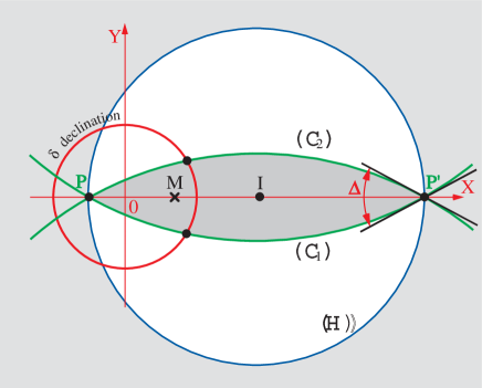
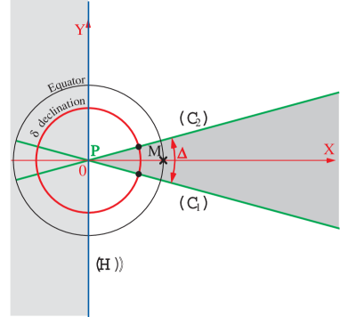
  Figure 7: (a) The projected lobe when the antenna is oriented North-South ($A=0^{\circ}$).
  (b) The particular case of the equatorial location ($\lambda=0^{\circ}$ and $A=0^{\circ}$).

  $\phi=\pi/2$ and (33) simplifies into

  $$\theta_{1}=\arctan\left[\frac{\cot(\Delta/2)}{\cos\lambda}\right]\pm\arccos\left[\frac{-\tan\delta\sin\lambda}{\sqrt{\cos^{2}\lambda+\cot^{2}(\Delta/2)}}\right]$$ (43)

  - If $\delta<\lambda-\pi/2$, the object is not visible.
  - If $\lambda-\pi/2<\delta<\pi/2-\lambda$, then the object enters the visibility lobe once per day during the exposure time

  $$t_{exp}=\frac{1\ day}{\pi}\left[-\arctan\left[\frac{\cot(\Delta/2)}{\cos\lambda}\right]+\arccos\left[\frac{-\tan\delta\sin\lambda}{\sqrt{\cos^{2}\lambda+\cot^{2}(\Delta/2)}}\right]\right]$$ (44)

  using the positive determinations for the $arctan$ and the $arccos$ in this expression.
  - If $\delta>\pi/2-\lambda$ and $\tan\delta<\frac{\sqrt{\cos^{2}\lambda+\cot^{2}(\Delta/2)}}{\sin\lambda}$, the object is circumpolar and enters the visibility lobe twice per day during the total exposure time given by:

  $$t_{exp}=\frac{1\ day}{\pi}\left[2\arccos\left[\frac{-\tan\delta\sin\lambda}{\sqrt{\cos^{2}\lambda+\cot^{2}(\Delta/2)}}\right]-\pi\right]$$

  $$=\frac{1\ day}{\pi}\left[\pi-2\arccos\left[\frac{\tan\delta\sin\lambda}{\sqrt{\cos^{2}\lambda+\cot^{2}(\Delta/2)}}\right]\right].$$ (45)

  - If $\tan\delta>\frac{\sqrt{\cos^{2}\lambda+\cot^{2}(\Delta/2)}}{\sin\lambda}$ (which is close to the condition $\delta>\pi/2-\Delta/2$ if $\Delta$ is small), the object is near the pole and is always in the visibility lobe.

• If $A=0$ and $\lambda=0$ (antenna on the equator), then the lobe is defined by two half-lines (Fig. 7b), and the full sky is visible with uniform daily exposures $t_{exp}=\Delta/2\pi\times 1\,sideral\,day$.

• $A=\pi/2$, antenna oriented East-West (Fig. 8a).
  

  

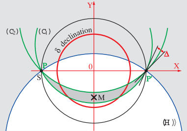
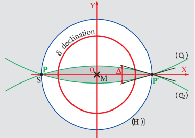
  Figure 8: (a) The projected lobe when the antenna is oriented East-West ($A=\pi/2$).
  (b) The particular case of the polar location ($\lambda=\pi/2$ and $A=\pi/2$).

  $\phi=\lambda$ and (33) simplifies into

  $$\theta_{1}=\pi/2\pm\arccos\left[\frac{-\tan\delta}{\tan(\lambda-\Delta/2)}\right]$$ (46)

  From Fig.8a we find that the visibility conditions are simply

  $$min(0,\lambda-\Delta/2)<\delta<\lambda+\Delta/2.$$

• $\lambda=\pi/2$ (antenna at the north pole).
  The lobe can be seen on Fig. 8b. $\phi=\pi/2$ and (33) simplifies into

  $$\theta_{1}=\pi/2\pm\arccos\left[-\tan\delta.\tan(\Delta/2)\right].$$ (47)

  If $\delta>\pi/2-\Delta/2$ then the object is always in the lobe; if $\delta<\pi/2-\Delta/2$ then the daily exposure is given by $t_{exp}=(1-\frac{2}{\pi}\arccos\left[\tan\delta\tan(\Delta/2)\right])\times(1\,sideral\,day)$.

5 Study of configurations

In this section, we study the impact of several orientations of a static cylindrical reflector on the field coverage and on the daily exposure time. BAO low-z studies should benefit from the widest coverage, favoured by the North-South ($A=0$) orientation of the cylinder axis; but high-z studies would need long exposures of low synchrotron background temperature fields, to allow deeper observations, a sensitivity that could be easier to reach with a different axis orientation.

Fig. 9 shows the map of foreground galactic synchrotron emission$\!{}^{{\bf?}}$ at $\sim 74cm$ .

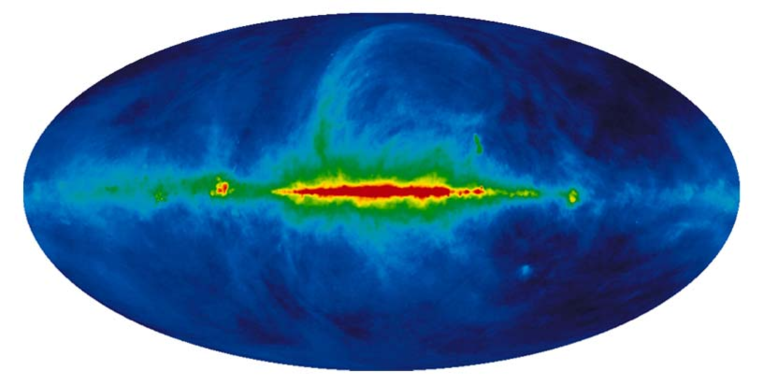
Figure 9: The Haslam map of the synchrotron galactic emission at 408 MHz (galactic coordinates).

This foreground has to be considered together with the exposure maps given below, in order to optimize the position and azimuth of the antenna.

5.1 Nançay

Fig. 10 (left) gives the exposure time for an antenna with a $\Delta=2^{\circ}$ lobe, located at Nançay (France) as a function of the galactic coordinates for different orientations. Fig. 10 (right) gives the field covered by the antenna with a daily exposure exceeding the abscissa-value and a sky synchrotron temperature lower than the ordinate-value.

• For $A=0^{\circ}$, 21500 square degree (52%) of the sky are covered with a daily exposure larger than 300s, and 2000 square degree (5%) are covered with an exposure larger than 1500s.

• For $A=45^{\circ}$, 17800 square degree (43%) of the sky are covered with a daily exposure larger than 300s, and 2800 square degree (7%) are covered with an exposure larger than 1500s.

• For $A=90^{\circ}$, 12200 square degree (30%) of the sky are covered with a daily exposure larger than 300s, and 3900 square degree (10%) are covered with an exposure larger than 1500s.

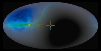
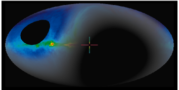
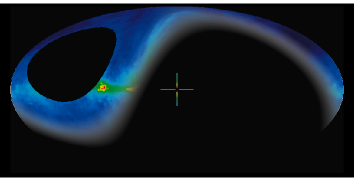
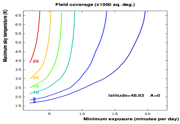
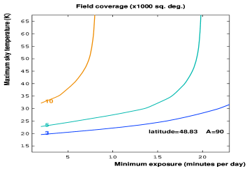
Figure 10: Antenna located at Nançay latitude (France). LEFT: Sky visibility (luminosity proportional to the Exposure time) as a function of galactic coordinates. From top to bottom: antenna azimuth $A=0^{\circ}$ (North-South), $A=45^{\circ}$ and $A=90^{\circ}$ (East-West). RIGHT: field covered by the antenna as a function of the minimum daily exposure and the maximum synchrotron sky temperature. For example, for $A=45^{\circ}$ (center), the point of coordinates $(15min.,30K)$ on the 3000 square degree curve means that 3000 square degrees of field with a sky background temperature below $30K$ transit during more than $15min.$ per sideral day in the instrumental lobe. These series of curves allows one to study the compromise between the field of view, the background level, and the exposure time.

5.2 Morocco

Fig. 11 (left) gives the exposure time for an antenna with a $\Delta=2^{\circ}$ lobe, located in central Morocco (latitude $33^{\circ}$) as a function of the galactic coordinates for different orientations. Fig. 11 (right) gives the field covered by the antenna with a daily exposure exceeding the abscissa-value and a sky synchrotron temperature lower than the ordinate-value.

• For $A=0^{\circ}$, 28200 square degree (68%) of the sky are covered with a daily exposure larger than 300s, and 1150 square degree (3%) are covered with an exposure larger than 1500s.

• For $A=45^{\circ}$, 22200 square degree (54%) of the sky are covered with a daily exposure larger than 300s, and 2100 square degree (5%) are covered with an exposure larger than 1500s.

• For $A=90^{\circ}$, 9600 square degree (23%) of the sky are covered with a daily exposure larger than 300s, and 4200 square degree (10%) are covered with an exposure larger than 1500s.

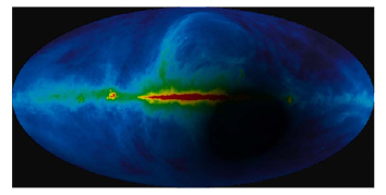
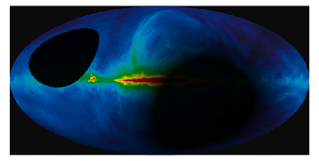
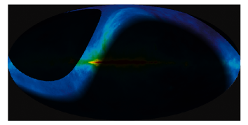
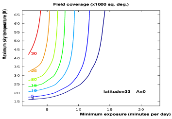
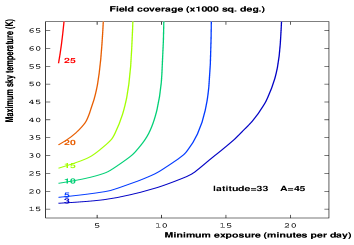
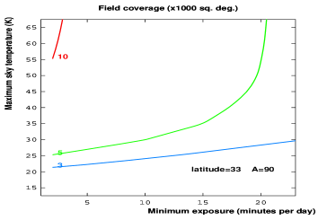
Figure 11: Antenna located in central Marocco latitude.
LEFT: Sky visibility (luminosity proportional to the Exposure time) as a function of galactic coordinates.
From top to bottom: antenna azimuth $A=0^{\circ}$ (North-South), $A=45^{\circ}$ and $A=90^{\circ}$ (East-West).
RIGHT: field covered by the antenna as a function of the minimum daily exposure and the maximum synchrotron sky temperature.

5.3 South Africa

Fig. 12 shows the exposure time and the field coverage for an antenna located at Hartebeesthoek Radio Astronomy Observatory (South Africa).

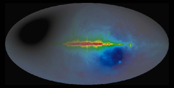
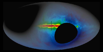
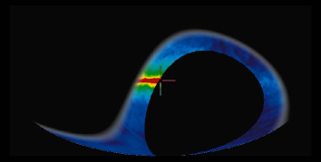
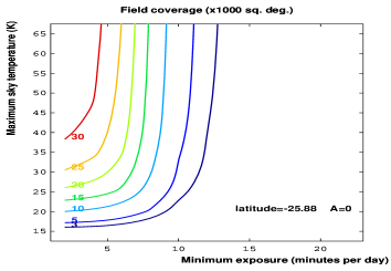
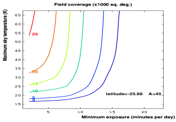
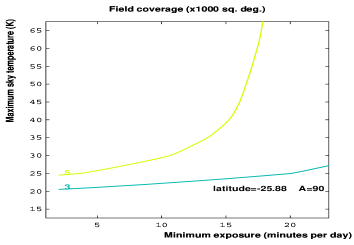
Figure 12: Antenna located at Hartebeesthoek Radio Astronomy Observatory latitude (South-Africa).
LEFT: Sky visibility (luminosity proportional to the Exposure time) as a function of galactic coordinates.
From top to bottom: antenna azimuth $A=0^{\circ}$ (North-South), $A=45^{\circ}$ and $A=90^{\circ}$ (East-West).
RIGHT: field covered by the antenna as a function of the minimum daily exposure and the maximum synchrotron sky temperature.

• For $A=0^{\circ}$, 31600 square degree (77%) of the sky are covered with a daily exposure larger than 300s, and 760 square degree (2%) are covered with an exposure larger than 1500s.

• For $A=45^{\circ}$, 24300 square degree (59%) of the sky are covered with a daily exposure larger than 300s, and 1600 square degree (4%) are covered with an exposure larger than 1500s.

• For $A=90^{\circ}$, 8100 square degree (20%) of the sky are covered with a daily exposure larger than 300s, and 4300 square degree (10%) are covered with an exposure larger than 1500s.

5.4 Equator

Fig. 13 shows the exposure time at the equator. In this case, the exposure time is uniform within the complete observable field, whatever be the azimuth of the antenna (but the observable field varies with $A$, see Fig. 13). For $A=0^{\circ}$, the daily exposure time is 480s on the full sky. For $A=45^{\circ}$, 29000 square degree (71%) of the sky are covered with a daily exposure time of 679s.

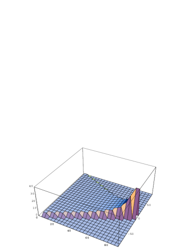
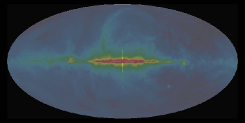
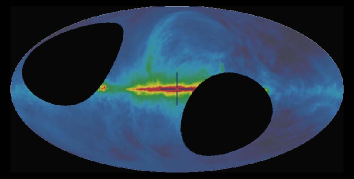
Figure 13: LEFT: the exposure time as a function of the antenna azimuth $A$ (from 0 to $90^{\circ}$) and the declination (from $-90^{\circ}$ to $90^{\circ}$) in the particular case of the equatorial location ($\lambda=0^{\circ}$). RIGHT: exposure time as a function of galactic coordinates when the antenna has azimuth $A=0^{\circ}$ (North-South, up) and $A=45^{\circ}$ (down).

6 Conclusions

The purpose of this study is to provide the exact expression of the transit time of a given celectial object within the lobe of a cylindrical reflector. Each particular case has been examined and the results have been used to analyse different telescope configurations. It is clear from this study that the groups planning to use a static setup of cylinders should seriously consider the orientation as a degree of freedom to favour either the largest field coverage with the shortest mean transit time (North-South orientation), or a smaller field coverage, but allowing a deeper survey (East-West orientation).

References

References

- [1] Peterson, J. B., Bandura, K., Pen, U. L., Jun. 2006. The Hubble Sphere Hydrogen Survey. arXiv:astro-ph/0606104.
- [2] R. Ansari, J.-E. Campagne, P. Colom, J.-M. Le Goff, C. Magneville, J. M. Martin, M. Moniez, J. Rich, and Ch. Yèche 2012. 21 cm observation of large-scale structures at : Instrument sensitivity and foreground subtraction. Astronomy and Astrophysics, 540, A129 (2012).
- [3] Bandura, K., Ph.D. thesis 2011 Pathfinder for a Neutral Hydrogen Dark Energy Survey. Carnegie Mellon University, 2011, 277 pages; AAT 3476113
- [4] Haslam, C-G-T., Salter, C-J., Stoffel, H., Wilson, W-E. 1982 A 408 MHz all-sky continuum survey. II - The atlas of contour maps. 1982, A& AS, 47, 1