Fast estimation of discretization error for FE problems solved by domain decomposition

Abstract

This paper presents a strategy for a posteriori error estimation for substructured problems solved by non-overlapping domain decomposition methods. We focus on global estimates of the discretization error obtained through the error in constitutive relation for linear mechanical problems. Our method allows to compute error estimate in a fully parallel way for both primal (BDD) and dual (FETI) approaches of non-overlapping domain decomposition whatever the state (converged or not) of the associated iterative solver. Results obtained on an academic problem show that the strategy we propose is efficient in the sense that correct estimation is obtained with fully parallel computations; they also indicate that the estimation of the discretization error reaches sufficient precision in very few iterations of the domain decomposition solver, which enables to consider highly effective adaptive computational strategies.

1 Introduction

The setting-up of robust numerical methods to solve complex systems of partial differential equations has become a key issue in applied mathematics and engineering, driven by the increasing use of numerical simulation in both research and industry. Among the latter, virtual testing has become a short term aim, with the objective to replace expensive experimental studies and validations by numerical simulations, even in order to certify large structures as planes and bridges.

Thus, one key point of the numerical methods to develop is the verification of computations which enables to warranty that the computed solution is sufficiently close to the original continuum mechanics model. This topic of numerical analysis has been the subject of many studies for the last decades. Three main classes of error estimator have been developed, based either on equilibrium residuals [1], flux projection [2] or error in constitutive law [3]. An overview of those various methods can be found in [4].

Another key point of numerical methods is their ability to quickly provide solutions to large (nonlinear) systems. The most classical answer to this issue is to use domain decomposition methods in order to take advantage of the parallel hardware architecture of recent clusters and grids. In engineering, non-overlapping domain decomposition methods are mostly employed, such as the well known FETI [5] or BDD [6]. An overview of the main approaches related to non-overlapping domain decomposition can be found in [7].

We aim to provide fully integrated adaptive strategies to compute large structural mechanics problems with certified quality. To do that, our current approach is to explore some ways of making bidirectional interactions between domain decomposition and a posteriori error estimation. Our developments are based both on the error in constitutive relation to measure the quality of our results and to forecast mesh refinement, and on a generic vision of non-overlapping domain decomposition methods which enables to do high-performance computing.

This paper focuses on the estimation of the global error in constitutive relation in order (among others) to study how it is influenced by the error in the convergence of the domain decomposition solver which is linked to the non-satisfaction of interface equations (continuity of displacements and balance of forces). To do so we propose a strategy to build, in parallel and during the iterations, displacement and stress fields which are kinematically admissible (KA) and statically admissible (SA) on the whole structure. We face two main difficulties. First, since before convergence interface fields do not possess the classical properties of discretized fields (continuity of displacements and weak equilibrium), the recovery of admissible displacements and stresses requires some preprocessing. Second, the computation of statically admissible fields being an operation which can not be conducted independently on each element (in some methods it can even be a large bandwidth operation), classical recovery methods [8, 9, 10, 11, 12, 13] would require inter-subdomain communications.

Our generic method to build continuous displacement and balanced traction fields for both primal and dual approaches of non-overlapping domain decomposition is presented through this paper. It will be shown that the properties of the preconditioners involved in domain decomposition solvers make this reconstruction costless, and that an error estimator can then be computed in a fully parallel way.

This paper is organized as follows. Section 2 recalls the general framework related to our upcoming developments, mainly the estimation of the error in constitutive equation and the use of domain decomposition method. Section 3 shows how the problem of error estimation in a substructured context can be brought back to the computation of nodal displacement and traction fields which are admissible in a discrete sense. Sections 4 and 5 describes how to obtain these fields without inter-subdomains exchanges when using classical primal (BDD) and dual (FETI) domain decomposition methods with good preconditioners. Section 6 presents numerical assessments, first to validate the parallel recovery procedure, then to prove that a good estimation can be obtained far earlier than the solver converged (in the sense of domain decomposition iterative solver). Finally, Section 7 concludes this paper.

2 Framework of the study

2.1 Reference mechanical problem

Let us consider the static equilibrium of a structure which occupies the open domain $\Omega\subset\mathbb{R}^{d}$ and which is submitted to given body forces $f$, to given traction forces $g$ on $\partial_{f}\Omega$ and to given displacements $u_{0}$ on the complementary part $\partial_{u}\Omega\neq\emptyset$. We assume the structure undergoes small perturbations and that the material is linear elastic, characterized by the Hooke’s tensor $\mathbb{H}$. Let $u$ be the unknown displacement field, $\varepsilon(u)$ the symmetric part of the gradient, $\sigma$ the Cauchy stress tensor.

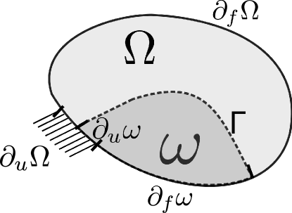
Figure 1: Domain $\Omega$, subdomain $\omega$ and boundaries

Let $\omega\subset\Omega$ be an open subset of $\Omega$, $\partial_{f}\omega=\partial\omega\cap\partial_{f}\Omega$, $\partial_{u}\omega=\partial\omega\cap\partial_{u}\Omega$ and $\Gamma=\partial\omega\setminus(\partial_{u}\omega\cup\partial_{f}\omega)$ (see Figure 1). We introduce two affine subspaces and one positive form:

• Subspace of kinematically admissible fields

  $${\mathrm{KA}}\!\left(\omega\right)=\left\{u\in\left(\mathrm{H}^{1}(\omega)\right)^{d},\ \operatorname{tr}(u)=u_{0}\text{ on }\partial_{u}\omega\right\}$$ (1)

  where $\operatorname{tr}$ is the trace operator.

• Subspace of statically admissible fields

  $$\mathop{\mathrm{SA}}\!\left(\omega\right)=\Bigg{\{}\tau\in\left(\mathrm{L}^{2}(\omega)\right)^{d\times d},\tau\text{ symmetric},\ \forall u^{*}\in{\mathrm{KA}}^{00}\!\left(\omega\right),\ \\ \int_{\omega}\tau:\varepsilon(u^{*})d\omega=\int_{\omega}f.u^{*}d\omega+\int_{\partial_{f}\omega}g.u^{*}dS\Bigg{\}}$$ (2)

  $$\text{where }{\mathrm{KA}}^{00}\!\left(\omega\right)=\left\{u\in\left(\mathrm{H}^{1}(\omega)\right)^{d},\ \operatorname{tr}(u)=0\text{ on }\partial_{u}\omega\cup\Gamma\right\}$$

• Measure of the non-verification of the constitutive equation [3]

  $$\mathop{\mathrm{e_{CR(\omega)}}}\!\left(u,\sigma\right)=\|\sigma-\mathbb{H}:\varepsilon\left(u\right)\|_{\mathbb{H}^{-1},\omega}$$ (3)

  where ${\|x\|_{\mathbb{H}^{-1},\omega}}=\displaystyle\sqrt{\int_{\omega}\left(x:{\mathbb{H}}^{-1}:x\right)d\omega}$

The mechanical problem set on $\Omega$ can be formulated as:

Find $\left(u_{ex},\sigma_{ex}\right)\in{\mathrm{KA}}\!\left(\Omega\right)\times\mathop{\mathrm{SA}}\!\left(\Omega\right)$ such that $\mathop{\mathrm{e_{CR(\Omega)}}}\!\left(u_{ex},\sigma_{ex}\right)=0$

2.2 Finite element approximation for the global problem

Let $\Omega_{h}$ be a tessellation of $\bar{\Omega}$ to which we associate a finite dimensional subspace $\mathrm{KA}_{h}\!\left(\Omega\right)$ of ${\mathrm{KA}}\!\left(\Omega\right)$. The classical finite element displacement approximation consists in searching

$$u_{h} \in\mathrm{KA}_{h}\!\left(\Omega\right)$$ (4)

$$\sigma_{h} =\mathbb{H}:\varepsilon(u_{h})$$

$$\int_{\Omega}\sigma_{h}:\varepsilon(u_{h}^{*})d\Omega =\int_{\Omega}f.u_{h}^{*}d\Omega+\int_{\partial_{f}\Omega}g.u_{h}^{*}dS,\qquad\forall u_{h}^{*}\in\mathrm{KA}_{h}^{00}\!\left(\Omega\right)$$

After introducing the $d\times N_{dof}$ matrix $\boldsymbol{\varphi}_{h}$ of shape functions which form a basis of $\mathrm{KA}_{h}\!\left(\Omega\right)$ and the vector of nodal unknowns $\mathbf{u}$ (of size $N_{dof}$, number of degrees of freedom) so that $u_{h}=\boldsymbol{\varphi}_{h}\mathbf{u}$, the classical finite element method leads to the well-known linear system:

$$\mathbf{K}\mathbf{u}=\mathbf{f}$$ (5)

where $\mathbf{K}$ is the (symmetric positive definite) stiffness matrix of domain $\Omega_{h}$ and $\mathbf{f}$ is the vector of generalized forces.

2.3 A posteriori error estimator

The finite element approximation $(u_{h},\sigma_{h})$ satisfies $u_{h}\in{\mathrm{KA}}\!\left(\Omega\right)$ and $\mathop{\mathrm{e_{CR(\Omega)}}}\!\left(u_{h},\sigma_{h}\right)=0$ but $\sigma_{h}\notin\mathop{\mathrm{SA}}\!\left(\Omega\right)$. The error in constitutive relation consists in deducing from $(u_{h},\sigma_{h})$ an admissible displacement-stress pair $(\widehat{u}_{h},\widehat{\sigma}_{h})\in{\mathrm{KA}}\!\left(\Omega\right)\times\mathop{\mathrm{SA}}\!\left(\Omega\right)$ in order to measure the residual on the constitutive equation (3) $\mathop{\mathrm{e_{CR(\Omega)}}}\!\left(\widehat{u}_{h},\widehat{\sigma}_{h}\right)\geqslant 0$. Using the well-known Prager-Synge theorem it can be proved that

$$\|\varepsilon(u_{ex})-\varepsilon(\widehat{u}_{h})\|_{\mathbb{H},\Omega}^{2}+\|\sigma_{ex}-\widehat{\sigma}_{h}\|_{\mathbb{H}^{-1},\Omega}^{2}=\left(\mathop{\mathrm{e_{CR(\Omega)}}}\!\left(\widehat{u}_{h},\widehat{\sigma}_{h}\right)\right)^{2}$$

Hence, the evaluation of the error in constitutive relation $\mathop{\mathrm{e_{CR(\Omega)}}}\!\left(\widehat{u}_{h},\widehat{\sigma}_{h}\right)$ for any admissible pair ($\widehat{u}_{h}$, $\widehat{\sigma}_{h}$) provides a guaranteed upper bound of the global error

$$\|\varepsilon(u_{ex})-\varepsilon(\widehat{u}_{h})\|_{\mathbb{H},\Omega}\leqslant\mathop{\mathrm{e_{CR(\Omega)}}}\!\left(\widehat{u}_{h},\widehat{\sigma}_{h}\right)$$ (6)

$\mathrm{KA}_{h}\!\left(\Omega\right)$ being a subspace of ${\mathrm{KA}}\!\left(\Omega\right)$, the construction of an admissible displacement field $\widehat{u}_{h}$ is straightforward since it can be taken equal to $u_{h}$. On the other hand, as $\sigma_{h}$ is not statically admissible, the construction of an admissible stress field $\widehat{\sigma}_{h}\in\mathop{\mathrm{SA}}\!\left(\Omega\right)$ is a crucial point which has already been widely studied in the literature. A first solution is to use a dual formulation of the reference problem [14] to compute $\widehat{\sigma}$ from scratch. Unfortunately building a subspace of $\mathop{\mathrm{SA}}\!\left(\Omega\right)$ is a complex task and most people prefer to post-process a statically admissible field from Field $\sigma_{h}$ obtained by a displacement formulation. Classical methods are the element equilibration techniques [8, 9], which have been improved by the use of the concept of partition of unity which lead to [11, 12, 13] and the flux-free method [10]. In most cases they involve the computation of efforts on “star-patches” which are the set of elements sharing one node, for each node of the mesh. Though rather simple these computations are in great number and thus expensive.

In the following, we note by $\mathcal{F}_{h}$ the algorithm which has been chosen to build an admissible stress field $\hat{\sigma}_{h}$. Whatever the choice, the algorithm takes as input not only the finite element stress field $\sigma_{h}$ but also the continuous representation of the imposed forces $(f,g)$.

$$\hat{\sigma}_{h}=\mathcal{F}_{h}(\sigma_{h},f,g)\in\mathop{\mathrm{SA}}\!\left(\Omega\right)$$

The algorithm we have used for our applications is the one proposed in [9] using a three degrees higher polynomial basis when solving the local problems on elements [15].

2.4 Substructured formulation

Let us consider a decomposition of domain $\Omega$ in open subsets $(\Omega^{(s)})_{1\leqslant s\leqslant N_{sd}}$ ($N_{sd}$ is the number of subdomains) so that $\Omega^{(s)}\cap\Omega^{(s^{\prime})}=\emptyset$ for $s\neq s^{\prime}$ and $\bar{\Omega}=\cup_{s}\bar{\Omega}^{(s)}$. Let $u^{\square}=(u^{(s)})_{s}$, we define the global assembling operator $\mathcal{A}$:

$$u=\mathcal{A}(u^{\square})\Leftrightarrow u_{|\Omega^{(s)}}=u^{(s)}$$ (7)

In order to reformulate the mechanical problem on the substructured configuration, we need to specify the conditions that should be satisfied at the boundary between subdomains $\Gamma^{(ss^{\prime})}=\partial\Omega^{(s)}\cap\partial\Omega^{(s^{\prime})}$. We have the fundamental properties:

$$\mathcal{A}(u^{\square})\in{\mathrm{KA}}\!\left(\Omega\right)\Leftrightarrow\left\{\begin{array}[]{l}u^{(s)}\in{\mathrm{KA}}\!\left(\Omega^{(s)}\right),\ \forall s\\ \operatorname{tr}(u^{(s)})=\operatorname{tr}(u^{(s^{\prime})})\text{ on }\Gamma^{(ss^{\prime})},\ \forall(s,s^{\prime})\end{array}\right.$$ (8)

$$\mathcal{A}(\sigma^{\square})\in\mathop{\mathrm{SA}}\!\left(\Omega\right)\Leftrightarrow\left\{\begin{array}[]{l}\sigma^{(s)}\in\mathop{\mathrm{SA}}\!\left(\Omega^{(s)}\right),\ \forall s\\ \sigma^{(s)}.n^{(s)}+\sigma^{(s^{\prime})}.n^{(s^{\prime})}=0\text{ on }\Gamma^{(ss^{\prime})},\ \forall(s,s^{\prime})\end{array}\right.$$ (9)

In other words, in order to be admissible on the whole domain $\Omega$, not only fields need to be admissible in a local sense (independently on each $\Omega^{(s)}$), but they also need to satisfy interface conditions, namely displacements continuity and tractions balance (action-reaction principle).

2.5 Finite element approximation for the substructured problem

We assume that the tessellation of $\bar{\Omega}$ and the substructuring are conforming so that (i) each element only belongs to one subdomain and (ii) nodes are matching on the interfaces. Each degree of freedom is either located inside a subdomain (subscript $i$) or on its boundary $\Gamma^{(s)}=\cup_{s^{\prime}}\Gamma^{(ss^{\prime})}$ (subscript $b$) where it is shared with at least one neighboring subdomain. Let $\boldsymbol{\lambda}_{b}^{(s)}$ be the vector of unknown efforts imposed on the interface of subdomain $\Omega^{(s)}_{h}$ by its neighbors. The finite element problem (5) can be written highlighting the contributions of subdomains:

$$\forall s,\ \mathbf{K}^{(s)}\mathbf{u}^{(s)}=\mathbf{f}^{(s)}+{\mathbf{t}^{(s)}}^{T}\boldsymbol{\lambda}_{b}^{(s)}\text{ with }\left\{\begin{array}[]{l}\sum\limits_{s}\mathbf{A}^{(s)}\boldsymbol{\lambda}_{b}^{(s)}=\mathbf{0}\\ \sum\limits_{s}\mathbf{\underline{A}}^{(s)}\mathbf{u}_{b}^{(s)}=\mathbf{0}\end{array}\right.$$ (10)

where $\mathbf{t}^{(s)}$ is the discrete trace operator ($\mathbf{u}^{(s)}_{b}=\mathbf{t}^{(s)}\mathbf{u}^{(s)}$) and where $\mathbf{A}^{(s)}$ and $\mathbf{\underline{A}}^{(s)}$ are assembling operators so that $\mathbf{A}^{(s)}$ enables to formulate the mechanical equilibrium of interfaces (9) and $\mathbf{\underline{A}}^{(s)}$ enables to formulate the continuity of displacements (8) (in the case of two subdomains, we have $\sum_{s}\mathbf{A}^{(s)}\boldsymbol{\lambda}_{b}=\boldsymbol{\lambda}_{b}^{(1)}+\boldsymbol{\lambda}_{b}^{(2)}=\mathbf{0}$ and $\sum_{s}\mathbf{\underline{A}}^{(s)}\mathbf{u}_{b}^{(s)}=\mathbf{u}_{b}^{(1)}-\mathbf{u}_{b}^{(2)}=\mathbf{0}$, see Fig. 7 for less trivial example and [7] for more an extensive description of all operators). One fundamental property of assembling operators is their orthogonality:

$$\sum_{s}\mathbf{\underline{A}}^{(s)}{\mathbf{A}^{(s)}}^{T}=\mathbf{0}$$ (11)

Note that the equilibrium of subdomain $\Omega^{(s)}$ also writes:

$$\begin{pmatrix}\mathbf{K}_{ii}^{(s)}&\mathbf{K}_{ib}^{(s)}\\ \mathbf{K}_{bi}^{(s)}&\mathbf{K}_{bb}^{(s)}\end{pmatrix}\begin{pmatrix}\mathbf{u}_{i}^{(s)}\\ \mathbf{u}_{b}^{(s)}\end{pmatrix}=\begin{pmatrix}\mathbf{f}_{i}^{(s)}\\ \mathbf{f}_{b}^{(s)}\end{pmatrix}+\begin{pmatrix}\mathbf{0}_{i}^{(s)}\\ \boldsymbol{\lambda}_{b}^{(s)}\end{pmatrix}$$ (12)

or in an equivalent condensed form:

$$\mathbf{S}^{(s)}\mathbf{u}_{b}^{(s)}=\mathbf{b}_{p}^{(s)}+\boldsymbol{\lambda}_{b}^{(s)}$$ (13)

with

$$\mathbf{S}^{(s)} =\mathbf{K}^{(s)}_{bb}-\mathbf{K}^{(s)}_{bi}{\mathbf{K}^{(s)}_{ii}}^{-1}\mathbf{K}^{(s)}_{ib}$$ (14)

$$\mathbf{b}^{(s)} =\mathbf{f}_{b}^{(s)}-\mathbf{K}^{(s)}_{bi}{\mathbf{K}^{(s)}_{ii}}^{-1}\mathbf{f}_{i}^{(s)}$$

where $\mathbf{S}^{(s)}$ is the Schur complement and $\mathbf{b}^{(s)}$ is the condensed right-hand side.

3 A posteriori error estimator in substructured context

The key point for the efficient evaluation of the error in constitutive relation in a substructured context (without overlapping) is to define admissible pairs ($\widehat{u}^{(s)}_{h}$,$\widehat{\sigma}^{(s)}_{h}$) $\in{\mathrm{KA}}\!\left(\Omega^{(s)}\right)\times\mathop{\mathrm{SA}}\!\left(\Omega^{(s)}\right)$ on each subdomain so that the associated assembled pair is admissible for the reference problem $(\mathcal{A}(\widehat{u}_{h}^{\square}),\mathcal{A}(\widehat{\sigma}_{h}^{\square}))\in{\mathrm{KA}}\!\left(\Omega\right)\times\mathop{\mathrm{SA}}\!\left(\Omega\right)$. Due to the absence of overlap, the additive structure of the associated error in constitutive relation leads to a fully parallel evaluation of the a posteriori error estimator:

$$\left(\mathop{\mathrm{e_{CR(\Omega)}}}\!\left(\mathcal{A}(\widehat{u}_{h}^{\square}),\mathcal{A}(\widehat{\sigma}_{h}^{\square})\right)\right)^{2}=\sum_{s}\left(\mathop{\mathrm{e_{CR(\Omega^{(s)})}}}\!\left(\widehat{u}^{(s)}_{h},\widehat{\sigma}^{(s)}_{h}\right)\right)^{2}$$

The application of a classical recovery strategy to compute admissible fields raises two difficulties in a substructured context. First, the star-patches can not be employed on the boundary nodes without assuming communication between subdomains. Though these exchanges would remain limited, we propose an alternate strategy to achieve full parallelism without impairing the properties of the error in constitutive relation. Second, in order to solve the substructured problem (10) parallel strategies consist in using iterative solvers which are based on the loosening of at least one of the interface conditions which is only verified (up to a certain precision) once the solver converged. Thus recovering strategies need to be adapted so that the local fields $(\widehat{u}_{h}^{(s)},\widehat{\sigma}_{h}^{(s)})$ satisfy the interface conditions.

The aim of this section is to prove that the determination of the admissible pair $(\mathcal{A}(\widehat{u}_{h}^{\square}),\mathcal{A}(\widehat{\sigma}_{h}^{\square}))$ can be brought back to the determination of nodal interface fields $(\widehat{\mathbf{u}}_{b}^{(s)},\widehat{\boldsymbol{\lambda}}_{b}^{(s)})_{s}$ which satisfy specific interface conditions. The construction of these nodal fields depends on the chosen domain decomposition strategy and is discussed in the following sections.

3.1 Kinematically admissible fields

In order to ensure interface Condition (8) when building $\widehat{u}^{(s)}_{h}\in{\mathrm{KA}}\!\left(\Omega^{(s)}\right)$ so that $\mathcal{A}(\widehat{u}_{h}^{\square})\in{\mathrm{KA}}\!\left(\Omega\right)$, we introduce continuous interface displacement fields $\hat{u}_{bh}^{(s)}$ from which we shall deduce internal displacement fields:

$$\hat{u}^{(s)}_{bh} =\hat{u}^{(s^{\prime})}_{bh}\ ,\ \forall(s,s^{\prime})$$

$$\hat{u}^{(s)}_{h|\Gamma^{(ss^{\prime})}} =\hat{u}^{(s)}_{bh},\ \forall s$$

Since discretizations are matching on the interface, the first condition can directly be imposed on finite element nodal quantities:

$${\widehat{\mathbf{u}}_{b}^{(s)}}={\widehat{\mathbf{u}}^{(s^{\prime})}_{b}}\ ,\ \forall(s,s^{\prime})$$

In order to deduce the internal fields, one finite element problem is solved independently on each subdomain with imposed Dirichlet conditions on the interface:

$${\widehat{\mathbf{u}}_{i}^{(s)}} ={\mathbf{K}^{(s)}_{ii}}^{-1}\left(\mathbf{f}_{i}^{(s)}-\mathbf{K}^{(s)}_{ib}{\mathbf{A}^{(s)}}^{T}\widehat{\mathbf{u}}_{b}^{(s)}\right)$$

$$\hat{u}_{h}^{(s)} =\boldsymbol{\varphi}_{h}^{(s)}\widehat{\mathbf{u}}^{(s)}=\begin{pmatrix}{\boldsymbol{\varphi}_{h}}_{{}_{i}}^{(s)}&{\boldsymbol{\varphi}_{h}}_{{}_{b}}^{(s)}\end{pmatrix}\begin{pmatrix}\widehat{\mathbf{u}}_{i}^{(s)}\\ \widehat{\mathbf{u}}_{b}^{(s)}\end{pmatrix}$$

$$\widehat{u} =\mathcal{A}(\widehat{u}_{h}^{\square})\in{\mathrm{KA}}\!\left(\Omega\right)$$

3.2 Statically admissible fields

In order to ensure interface Condition (9) when building $\widehat{\sigma}^{(s)}_{h}\in\mathop{\mathrm{SA}}\!\left(\Omega^{(s)}\right)$ so that $\mathcal{A}(\widehat{\sigma}_{h}^{\square})\in\mathop{\mathrm{SA}}\!\left(\Omega\right)$, we introduce for each subdomain the continuous balanced interface traction fields $\widehat{F}_{bh}^{(s)}$ defined on $\Gamma^{(s)}$ which satisfy:

$$\widehat{\sigma}_{h}^{(s)}.n^{(s)} =\widehat{F}_{bh}^{(s)}\text{ on }\Gamma^{(s)}$$ (15)

$$\widehat{F}_{bh}^{(s)}+\widehat{F}_{bh}^{(s^{\prime})} =0\text{ on }\Gamma^{(ss^{\prime})}$$

$$\int_{\Omega^{(s)}}f.\rho d\Omega+\int_{\partial_{f}\Omega^{(s)}}g^{(s)}.\rho dS+\int_{\Gamma^{(s)}}\widehat{F}_{bh}^{(s)}.\rho dS =0\quad\forall\rho\in\mathrm{RKA}^{0}(\Omega^{(s)})$$

where $\mathrm{RKA}^{0}(\Omega^{(s)})$ is the set of rigid body motions which are compatible with Dirichlet conditions imposed on $\partial_{u}\Omega^{(s)}$:

$$\mathrm{RKA}^{0}(\Omega^{(s)})=\left\{\rho\in\mathrm{H}^{1}(\Omega^{(s)}),\ \rho=0\text{ on }\partial_{u}\Omega^{(s)},\ \varepsilon(\rho)=0,\right\}$$

The last condition of (15) is the translation of Fredholm’s alternative in order to ensure the well-posedness of the static problem on domain $\Omega^{(s)}$. To build these traction fields in a simple way, we associate them with the finite element nodal reaction field ${\widehat{\boldsymbol{\lambda}}}^{(s)}_{b}$:

$$\int_{\Gamma^{(ss^{\prime})}}\widehat{F}_{bh}^{(s)}\cdot{\varphi_{j}^{(s)}}_{|\Gamma^{(ss^{\prime})}}dS={\widehat{\boldsymbol{\lambda}}}_{b,j}^{(s)}$$ (16)

where $j$ denote a node of the interface, $\varphi_{j}^{(s)}$ its associated shape function and ${\widehat{\boldsymbol{\lambda}}}^{(s)}_{b,j}$ the corresponding nodal component of ${\widehat{\boldsymbol{\lambda}}}^{(s)}_{b}$. This equation then imposes that the discrete field ${\widehat{\boldsymbol{\lambda}}}_{b}^{(s)}$ and the continuous field $\widehat{F}_{bh}^{(s)}$ develop the same virtual work in any finite element displacement field. The conditions on $\widehat{F}_{bh}^{(s)}$ have these discrete counterparts on ${\widehat{\boldsymbol{\lambda}}}^{(s)}_{b}$:

$$\sum\limits_{s}\mathbf{A}^{(s)}\widehat{\boldsymbol{\lambda}}_{b}^{(s)} =\mathbf{0}$$ (17)

$${\mathbf{R}^{(s)}}^{T}\left({\mathbf{t}^{(s)}}^{T}{\widehat{\boldsymbol{\lambda}}}_{b}^{(s)}+\mathbf{f}^{(s)}\right) =\mathbf{0}$$

where $\mathbf{R}^{(s)}$ is a basis of $\ker(\mathbf{K}^{(s)})$. As said earlier, the first equation corresponds to the equilibrium between subdomains. The second equation corresponds to the balance of the subdomain with respect to virtual rigid body motions (since this kind of displacement field is exactly represented in the finite element approximation, the discrete condition is equivalent to the continuous one).

As a first approach, we define $\widehat{F}_{bh}^{(s)}$ as:

$$\widehat{F}_{bh}^{(s)}=\boldsymbol{\varphi}_{h}{}_{|\Gamma^{(s)}}^{(s)}{\widehat{\mathbf{F}}}_{b}^{(s)}$$ (18)

where ${\widehat{\mathbf{F}}}_{b}^{(s)}$ is the vector of nodal values of $\widehat{F}_{bh}^{(s)}$ and $\boldsymbol{\varphi}_{h}{}_{|\Gamma^{(s)}}^{(s)}$ refers to the vector of the trace on $\Gamma^{(s)}$ of finite element shape functions. Vector ${\widehat{\mathbf{F}}}_{b}^{(s)}$ is then obtained by the inversion of the (small) “mass” matrix of the interface of each subdomain. In the following, we denote by $\mathcal{G}_{h}$ the previous procedure which associates a continuous balanced interface force $\widehat{F}_{bh}^{(s)}$ to a balanced nodal interfaces forces ${\widehat{\boldsymbol{\lambda}}}^{(s)}_{b}$:

$$\widehat{F}_{bh}^{(s)}=\mathcal{G}_{h}({\widehat{\boldsymbol{\lambda}}}^{(s)}_{b})$$ (19)

The traction field $\widehat{F}_{bh}^{(s)}$ allows to satisfy the interface conditions associated to the static admissibility. The next step is to build internal finite element stress fields which match the associated nodal boundary field ${\widehat{\boldsymbol{\lambda}}}^{(s)}_{b}$. This is done by solving one finite element problem on each subdomain with imposed Neumann conditions on the interface.

$$\tilde{\mathbf{u}}^{(s)} ={\mathbf{K}^{(s)}}^{+}\left(\mathbf{f}^{(s)}+{\mathbf{t}^{(s)}}^{T}{\widehat{\boldsymbol{\lambda}}}^{(s)}_{b}\right)$$ (20)

$$\widehat{\sigma}_{h}^{(s)} =\mathcal{F}_{h}\left(\mathbb{H}:\varepsilon(\boldsymbol{\varphi}_{h}^{(s)}\tilde{\mathbf{u}}^{(s)}),f^{(s)},\left\{g^{(s)},\mathcal{G}_{h}({\widehat{\boldsymbol{\lambda}}}^{(s)}_{b})\right\}\right)$$

$$\widehat{\sigma}_{h} =\mathcal{A}(\widehat{\sigma}_{h}^{\square})\in\mathop{\mathrm{SA}}\!\left(\Omega\right)$$

The use of the pseudo-inverse ${\mathbf{K}^{(s)}}^{+}$ is due to the potential lack of Dirichlet boundary conditions on the substructure. Displacement field $\tilde{\mathbf{u}}^{(s)}$ is defined up to a rigid body motion which needs not to be determined since only the symmetric gradient of the associated displacement field is required.

It has to be noted that the fully parallel procedure $\mathcal{G}_{h}$ proposed above leads to a different admissible traction field as would have been obtained using standard patch-technique [9] (referred in the sequel as the sequential approach). Thus the use of $\mathcal{G}_{h}$ implies that the parallel error estimation is different from the standard sequential one even when discrete interface conditions are satisfied. For now there are no theoretical results on the quality of the resulting fields, examples (as given in Section 6) show that sequential estimator and parallel estimator (when interface conditions have sufficiently converged, which happens very quickly) can not be distinguished.

4 Recovery of admissible fields in BDD

In the Balancing domain decomposition [16, 17], a unique interface displacement unknown $\mathbf{u}_{b}$ is introduced so that continuity is always insured:

$$\mathbf{u}_{b}^{(s)}={\mathbf{A}^{(s)}}^{T}\mathbf{u}_{b}\Longrightarrow\sum_{s}\mathbf{\underline{A}}^{(s)}\mathbf{u}_{b}^{(s)}=\mathbf{0}$$ (21)

Other quantities can be deduced from $\mathbf{u}_{b}$ and equations (12,13):

$$\mathbf{u}_{i}^{(s)} ={\mathbf{K}^{(s)}_{ii}}^{-1}\left(\mathbf{f}_{i}^{(s)}-\mathbf{K}^{(s)}_{ib}{\mathbf{A}^{(s)}}^{T}\mathbf{u}_{b}\right)$$ (22)

$$\boldsymbol{\lambda}_{b}^{(s)} =\mathbf{S}^{(s)}\mathbf{u}_{b}-\mathbf{b}^{(s)}$$

The BDD solver consists in iteratively finding the interface displacement $\mathbf{u}_{b}$ which insure global equilibrium ($\sum_{s}\mathbf{A}^{(s)}\boldsymbol{\lambda}^{(s)}_{b}=\mathbf{0}$),

$$\mathbf{0}=\sum_{s}\mathbf{A}^{(s)}\boldsymbol{\lambda}_{b}^{(s)}=\left(\sum_{s}\mathbf{A}^{(s)}\mathbf{S}^{(s)}{\mathbf{A}^{(s)}}^{T}\right)\mathbf{u}_{b}-\left(\sum_{s}\mathbf{A}^{(s)}\mathbf{b}^{(s)}\right)$$ (23)

4.1 Recovery of KA fields

In the BDD solver, kinematic interface conditions are satisfied anytime and using $\widehat{\mathbf{u}}_{b}^{(s)}=\mathbf{u}_{b}$ enables to build $\widehat{u}^{(s)}_{h}$ so that $\widehat{u}_{h}=\mathcal{A}\left(\widehat{u}_{h}^{\square}\right)\in{\mathrm{KA}}\!\left(\Omega\right)$. Note that all associated computations are realized during the standard resolution process so that no extra operation is required.

4.2 Recovery of SA fields

For a given interface displacement $\mathbf{u}_{b}$, we note:

$$\llceil\boldsymbol{\lambda}_{b}\rrceil=\sum_{s}\mathbf{A}^{(s)}\boldsymbol{\lambda}^{(s)}_{b}=\sum_{s}\mathbf{A}^{(s)}\left(\mathbf{S}^{(s)}\mathbf{u}_{b}-\mathbf{b}^{(s)}\right)$$

Obviously $\llceil\boldsymbol{\lambda}_{b}\rrceil$ is zero if and only if $\mathbf{u}_{b}$ is the solution to (23). We then define:

$${\widehat{\boldsymbol{\lambda}}}^{(s)}_{b}=\boldsymbol{\lambda}^{(s)}_{b}-\left.\tilde{\mathbf{A}}^{(s)}\right.^{T}\llceil\boldsymbol{\lambda}_{b}\rrceil$$ (24)

where $(\tilde{\mathbf{A}}^{(s)})_{s}$ are scaled assembling operators so that $\sum_{s}\mathbf{A}^{(s)}\left.\tilde{\mathbf{A}}^{(s)}\right.^{T}=\mathbf{I}$. The multiplicity scaling is a typical example of such operator $\tilde{\mathbf{A}}^{(s)}$:

$$\left.\tilde{\mathbf{A}}^{(s)}\right.^{T}=\left.\mathbf{A}^{(s)}\right.^{T}\left(\sum_{j}\mathbf{A}^{(j)}\left.\mathbf{A}^{(j)}\right.^{T}\right)^{-1}$$

which, in the case of two subdomains, gives $\left.\tilde{\mathbf{A}}^{(s)}\right.^{T}\llceil\boldsymbol{\lambda}_{b}\rrceil=\displaystyle\frac{1}{2}\llceil\boldsymbol{\lambda}_{b}\rrceil$. In the case of heterogeneous structures, other scaled assembly operators which take the heterogeneity into account are used [18, 19, 20].

It is clear that by definition, $\widehat{\boldsymbol{\lambda}}^{(s)}_{b}$ is a balanced nodal reaction field:

$$\sum_{s}\mathbf{A}^{(s)}{\widehat{\boldsymbol{\lambda}}}^{(s)}_{b}=0$$

In order to prove that ${\widehat{\boldsymbol{\lambda}}}^{(s)}_{b}$ also satisfies Fredholm’s alternative, we note that since $\mathbf{R}^{(s)}$ is a basis of $\mathrm{ker}(\mathbf{K}^{(s)})$ and $\mathbf{K}_{ii}^{(s)}$ is invertible, we have $\mathbf{S}^{(s)}\mathbf{R}^{(s)}_{b}=\mathbf{0}$ and $\mathbf{R}^{(s)}_{i}=-\left.\mathbf{K}_{ii}^{(s)}\right.^{-1}\mathbf{K}_{ib}^{(s)}\mathbf{R}^{(s)}_{b}$. The condition then writes in an equivalent condensed form:

$$\left.\mathbf{R}^{(s)}_{b}\right.^{T}\left({\widehat{\boldsymbol{\lambda}}}^{(s)}_{b}+\mathbf{b}^{(s)}\right) =0$$

$$\left.\mathbf{R}^{(s)}_{b}\right.^{T}\left(\mathbf{S}^{(s)}\mathbf{u}_{b}-\mathbf{b}^{(s)}+\left.\tilde{\mathbf{A}}^{(s)}\right.^{T}\llceil\boldsymbol{\lambda}_{b}\rrceil+\mathbf{b}^{(s)}\right) =0$$

Using the symmetry of $\mathbf{S}^{(s)}$ (inherited from the symmetry of $\mathbf{K}^{(s)}$) to nullify $\left.\mathbf{R}^{(s)}_{b}\right.^{T}\mathbf{S}^{(s)}$, the condition writes:

$$\left(\tilde{\mathbf{A}}^{(s)}\mathbf{R}^{(s)}_{b}\right)^{T}\llceil\boldsymbol{\lambda}_{b}\rrceil=0$$ (25)

which is exactly the balancing condition [6] of the iterative BDD solver: the residual of the BDD iterative solver $\llceil\boldsymbol{\lambda}_{b}\rrceil=\left(\sum_{s}\mathbf{A}^{(s)}\boldsymbol{\lambda}^{(s)}_{b}\right)$ (23) has to be orthogonal to all local weighted rigid body motions so that preconditioning step is well posed.

Then we have constructed a pair of interface nodal Vectors $(\widehat{\mathbf{u}}_{b},\widehat{\boldsymbol{\lambda}}_{b})$ which satisfy all required conditions to build admissible fields.

Note that all the involved operations are already realized during classical steps of the primal domain decomposition approach with a Neumann-Neumann preconditioner and the associated coarse problem, so that all finite element quantities (even the internal ones) are available at no cost; the only extra operations are due to the use of Algorithms $\mathcal{G}_{h}$ (to compute $\widehat{F}_{bh}$) and $\mathcal{F}_{h}$ (to compute $\widehat{\sigma}_{h}$).

5 Recovery of admissible fields in FETI

In the Finite Element Tearing and Interconnecting domain decomposition [5], a unique interface effort unknown $\boldsymbol{\lambda}_{b}$ is introduced so that interface equilibrium is always insured:

$$\boldsymbol{\lambda}_{b}^{(s)}={\mathbf{\underline{A}}^{(s)}}^{T}\boldsymbol{\lambda}_{b}\Longrightarrow\sum_{s}\mathbf{A}^{(s)}\boldsymbol{\lambda}_{b}^{(s)}=\mathbf{0}$$ (26)

Displacements can be deduced from $\boldsymbol{\lambda}_{b}$ if it satisfies Fredholm’s alternative on each substructure:

$$\mathbf{u}^{(s)} ={\mathbf{K}^{(s)}}^{+}\left(\mathbf{f}^{(s)}+{\mathbf{t}^{(s)}}^{T}{\mathbf{\underline{A}}^{(s)}}^{T}\boldsymbol{\lambda}_{b}\right)+\mathbf{R}^{(s)}\boldsymbol{\alpha}^{(s)}$$ (27)

$$\mathbf{0} ={\mathbf{R}^{(s)}}^{T}\left(\mathbf{f}^{(s)}+{\mathbf{t}^{(s)}}^{T}{\mathbf{\underline{A}}^{(s)}}^{T}\boldsymbol{\lambda}_{b}\right)$$

where $\boldsymbol{\alpha}^{(s)}$ is the unknown magnitude of rigid body motions. The FETI solver consists in iteratively finding an interface effort $\boldsymbol{\lambda}_{b}$, under the previous constraint, which insures the continuity of interface displacement:

$$\mathbf{0}=\sum_{s}\mathbf{\underline{A}}^{(s)}\mathbf{u}_{b}^{(s)}=\left(\sum_{s}\mathbf{\underline{A}}^{(s)}\mathbf{t}^{(s)}{\mathbf{K}^{(s)}}^{+}{\mathbf{t}^{(s)}}^{T}{\mathbf{\underline{A}}^{(s)}}^{T}\right)\boldsymbol{\lambda}_{b}\\ +\left(\sum_{s}\mathbf{\underline{A}}^{(s)}\mathbf{t}^{(s)}{\mathbf{K}^{(s)}}^{+}\mathbf{f}^{(s)}\right)+\left(\sum_{s}\mathbf{\underline{A}}^{(s)}\mathbf{t}^{(s)}\mathbf{R}^{(s)}\boldsymbol{\alpha}^{(s)}\right)$$ (28)

5.1 Recovery of SA fields

In the FETI solver, the nodal interface fields ${\boldsymbol{\lambda}}^{(s)}_{b}={\mathbf{\underline{A}}^{(s)}}^{T}\boldsymbol{\lambda}_{b}$ are by construction always balanced at the interface (26) and associated to well-posed discrete Neumann problems on each substructure (27). Hence, we can directly set $\widehat{\boldsymbol{\lambda}}_{b}^{(s)}={\boldsymbol{\lambda}}^{(s)}_{b}$ and apply algorithms $\mathcal{G}_{h}$ and $\mathcal{F}_{h}$ to compute $\widehat{\sigma}^{(s)}_{h}\in\mathop{\mathrm{SA}}\!\left(\Omega^{(s)}\right)$ with $\widehat{\sigma}_{h}=\mathcal{A}(\widehat{\sigma}_{h}^{\square})\in\mathop{\mathrm{SA}}\!\left(\Omega\right)$.

5.2 Recovery of KA fields

For a given balanced nodal interface traction $\boldsymbol{\lambda}_{b}$, we introduce, in agreement with (27), the gap of the interface displacement :

$$\llfloor\mathbf{u}_{b}\rrfloor=\sum_{s}\mathbf{\underline{A}}^{(s)}\mathbf{u}^{(s)}_{b}$$

and we define

$$\widehat{\mathbf{u}}^{(s)}_{b}=\mathbf{u}^{(s)}_{b}-\left.\tilde{\mathbf{\underline{A}}}^{(s)}\right.^{T}\llfloor\mathbf{u}_{b}\rrfloor$$

where $(\tilde{\mathbf{\underline{A}}}^{(s)})_{s}$ are scaled assembling operators so that $\sum_{s}\mathbf{\underline{A}}^{(s)}\left.\tilde{\mathbf{\underline{A}}}^{(s)}\right.^{T}=\mathbf{I}$. Similarly to the BDD case, a typical example of such operator $\tilde{\mathbf{\underline{A}}}^{(s)}$ is the multiplicity scaling:

$$\left.\tilde{\mathbf{\underline{A}}}^{(s)}\right.^{T}=\left.\mathbf{\underline{A}}^{(s)}\right.^{T}\left(\sum_{j}\mathbf{\underline{A}}^{(j)}\left.\mathbf{\underline{A}}^{(j)}\right.^{T}\right)^{-1}$$ (29)

Note that in the case of two subdomains, we have: $\left.\tilde{\mathbf{\underline{A}}}^{(s)}\right.^{T}\llfloor\mathbf{u}_{b}\rrfloor=\displaystyle\frac{1}{2}\llfloor\mathbf{u}_{b}\rrfloor$. The connection between FETI and BDD scaling operators (even in the heterogeneous case) is given in [21].

It is clear that by construction

$$\sum_{s}\mathbf{\underline{A}}^{(s)}\widehat{\mathbf{u}}^{(s)}_{b}=\mathbf{0}$$

Hence nodal interface displacement $\widehat{\mathbf{u}}^{(s)}_{b}$ can be used to deduce an admissible displacement field $\widehat{u}^{(s)}_{h}$ so that $\widehat{u}_{h}=\mathcal{A}\left(\widehat{u}_{h}^{\square}\right)\in{\mathrm{KA}}\!\left(\Omega\right)$.

Then we have constructed a pair of interface nodal Vectors $(\widehat{\mathbf{u}}_{b},\widehat{\boldsymbol{\lambda}}_{b})$ which satisfies all required conditions to build admissible fields. Note that all the involved operations are already realized during classical steps of the dual domain decomposition approach (with built-in coarse problem) with Dirichlet’s preconditioner, so that all finite element quantities (even the internal ones) are available at no cost: the quantity $\llfloor\mathbf{u}_{b}\rrfloor$ is directly available during the classical solution procedure (without computing any $\boldsymbol{\alpha}^{(j)}$) which is based on an initialization/projection algorithm [5], and the displacement field ${\mathbf{u}}^{(s)}$ can be defined up to an element of the kernel (a rigid body motion) since only its symmetric gradient is used during the computation of the error. The only extra operations are due to the use of algorithms $\mathcal{G}_{h}$ (to compute $\widehat{F}_{bh}$) and $\mathcal{F}_{h}$ (to compute $\widehat{\sigma}_{h}$).

6 Numerical assessment

In order to assess the performance of our parallel error estimator, we consider the 2D toy problem of the $\Gamma$-shape structure of Figure 2(a) which has been used in other papers like [22]. Plane stresses are assumed. The material behavior is isotropic, linear and elastic, with Young modulus $E=2000$ MPa and Poisson’s ratio $\nu=0.3$. The structure is clamped on its basis (whose length is denoted $L$) and it is submitted to traction and shear on its upper-right side, while all the remaining boundaries are traction-free.

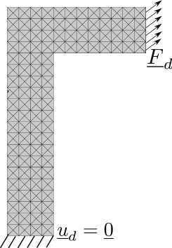
(a) Finite element problem ($h=~{}\frac{L}{4})$

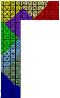
(b) Substructuring ($h=~{}\frac{L}{8}$, $N_{sd}=8$)

Figure 2: $\Gamma$-shape structure

Several regular meshes have been generated, constituted by triangular elements of characteristic size $h=\frac{L}{m}$ with $m=2,4,8,16,32$. For each mesh, a sequential (mono-domain) computation is driven, followed by domain decomposition computations obtained by an automatic splitting of the mesh in an increasing number $N_{sd}$ of subdomains ( $N_{sd}=2,4,8$ when $m\leqslant 4$ and $N_{sd}=2,4,8,16,32$ when $m\geqslant 8$). Figure 2(b) shows such a decomposition for $N_{sd}=8$ and $m=8$.

All the computations are driven in the ZeBuLoN finite element code [23], using elements of polynomial degree $p=1$. Both BDD and FETI algorithms are used to solve the substructured problems, respectively used together with Neumann-Neumann and Dirichlet preconditioners. Beside, the convergence criterion of the solver, which stands here for the interface traction gap (resp. displacement gap) in the primal (resp. dual) approach, is set to $10^{-6}$.

On each case, in addition to the new parallel error estimator $\mathrm{e_{CR}^{ddm}}$, we compute the standard sequential $\mathrm{e_{CR}^{seq}}$ and the true error $e_{h}$ obtained using a reference field $u_{ex}$ computed on a very fine mesh:

$$\mathrm{e_{CR}^{seq}} =\mathop{\mathrm{e_{CR(\Omega)}}}\!\left(\widehat{u}_{h},\widehat{\sigma}_{h}\right)$$

$$\mathrm{e_{CR}^{ddm}} =\sqrt{\sum_{s}\left(\mathop{\mathrm{e_{CR(\Omega^{(s)})}}}\!\left(\widehat{u}^{(s)}_{h},\widehat{\sigma}^{(s)}_{h}\right)\right)^{2}}$$

$$e_{h} =\|\varepsilon\left(u_{ex}-\hat{u}_{h}\right)\|_{\mathbb{H},\Omega}=\sqrt{{\|\varepsilon\left(u_{ex}\right)\|_{\mathbb{H},\Omega}^{2}}-{\|\varepsilon\left(\hat{u}_{h}\right)\|_{\mathbb{H},\Omega}^{2}}}$$

6.1 Quality of the parallel error estimator

We first study the quality of the parallel error estimator $\mathrm{e_{CR}^{ddm}}$ for computations when convergence of the domain decomposition solver is reached. As said earlier, the proposed technique does not lead to the same statically admissible field because of the special treatment of the interface traction (19). Our estimator might then be sensitive to the substructuring, we thus compare the estimations obtained with meshes of characteristic size $h$ and decomposition into $N_{sd}$ subdomains. Results are given in Figure 3 and Table 1.

Figure 3: Convergence of Error $e_{h}$ and Estimators $\mathrm{e_{CR}^{seq}}$ and $\mathrm{e_{CR}^{ddm}}$ (for various $N_{sd}$) vs. element size $h$

$h$	$L/2$	$L/4$	$L/8$	$L/16$	$L/32$
$\#$ dofs	146	514	1922	7426	29186
$e_{h}$	0.2347	0.1493	0.0937	0.0597	0.0386
$\mathrm{e_{CR}^{seq}}$	0.5712	0.4035	0.2662	0.1769	0.1151
$N_{sd}$	$\mathrm{e_{CR}^{ddm}}$
2	0.5657	0.4021	0.2648	0.1747	0.1151
4	0.5768	0.4007	0.2648	0.1747	0.1151
8	0.5546	0.4007	0.2676	0.1747	0.1165
16			0.2690	0.1761	0.1165
32			0.2787	0.1789	0.1178

Table 1: Error $e_{h}$ and Estimators $\mathrm{e_{CR}^{seq}}$ and $\mathrm{e_{CR}^{ddm}}$ (for various $N_{sd}$) vs. element size $h$

We observe that:

• The results obtained by FETI and BDD can not be distinguished (which is why only FETI results are given in Table 1).

• $\mathrm{e_{CR}^{ddm}}$ barely depends on the substructuring; the results are quite similar whether they are conducted on a single domain (“sequential” curve) or on $N_{sd}$ subdomains. Only a slight rise of the estimation can be observed when the number of interface degrees of freedom is not small compared to the number of internal degrees of freedom, which is logical since the description of interface traction fields is coarser in parallel than in sequential.

As a conclusion, the parallel error estimator $\mathrm{e_{CR}^{ddm}}$ enables to recover the same efficiency factor as the standard sequential one, while the CPU-time is divided by $N_{sd}$.

6.2 Convergence of the parallel estimator along DD-solver iterations

Previous results enabled to analyse the quality of the parallel estimator when interface quantities had converged. A new feature associated to the use of an iterative solver for the domain decomposition (DD) problem is that the discretization error estimation can be conducted before DD convergence is reached, that is in presence of displacement or traction discontinuity at the interface as explained in Sections 4 and 5

We then compute the parallel error estimator $\mathrm{e_{CR}^{ddm}}$ at each iteration of the DD solver. Convergence curves of $\mathrm{e_{CR}^{ddm}}$ during the FETI and BDD iterations are shown on Figure 4. Parallel error estimator is plotted as a function of the FETI (resp. BDD) residual, defined (for Iteration $n$) as the normalized displacement (resp. traction) gap at the interface:

$$r^{n}=\frac{\llfloor\mathbf{u}_{b}^{n}\rrfloor_{\Gamma}}{\llfloor\mathbf{u}_{b}^{0}\rrfloor_{\Gamma}}\qquad\text{ or }\qquad r^{n}=\frac{\llceil\boldsymbol{\lambda}_{b}^{n}\rrceil_{\Gamma}}{\llceil\boldsymbol{\lambda}_{b}^{0}\rrceil_{\Gamma}}$$ (30)

Classical stopping criterion for the of convergence of DD solver is this residual being below $10^{-6}$. Because of the similarity between the curves, the only shown cases correspond to $h=L/8$ and $h=L/16$.

\psfrag{error estimator}{$\mathrm{e_{CR}^{ddm}}$}\includegraphics[width=201.6317pt]{D_error_gap_h08}	\psfrag{error estimator}{$\mathrm{e_{CR}^{ddm}}$}\includegraphics[width=201.6317pt]{D_error_gap_h16}
FETI Case: $h=L/8$	FETI Case: $h=L/16$
\psfrag{error estimator}{$\mathrm{e_{CR}^{ddm}}$}\includegraphics[width=201.6317pt]{P_error_gap_h08}	\psfrag{error estimator}{$\mathrm{e_{CR}^{ddm}}$}\includegraphics[width=201.6317pt]{P_error_gap_h16}
BDD Case: $h=L/8$	BDD Case: $h=L/16$

Figure 4: Convergence of estimator vs. DD residual

The curves show a rapid convergence of the parallel error estimator along iterations of the solver, so that $\mathrm{e_{CR}^{ddm}}$ can be considered as converged when FETI residual reaches an order of magnitude of $5.10^{-3}$ or BDD residual reaches $5.10^{-1}$, which corresponds to at most 5 iterations whereas the solver convergence is achieved in 10 to 20 iterations.

Actually, $\mathrm{e_{CR}^{ddm}}$ is driven by both the discretization error and the convergence of the solver (interface error). The “L”-shaped curves show that the impact of residual of the DD solver is preponderant only at the first iterations (when interface fields are very poorly estimated), after $\mathrm{e_{CR}^{ddm}}$ stagnates at a value very close to $\mathrm{e_{CR}^{seq}}$ which is only associated to the discretization error.

Then, it seems possible to stop the iterations of the solver far before convergence while still obtaining an accurate global estimate for the discretization error.

Figures 5 and 6 show maps of the elementary contributions $\mathrm{e_{CR}^{ddm,E}}$ to the parallel error estimator $\mathrm{e_{CR}^{ddm}}$ at different steps of the convergence, for $N_{sd}=8$ with $h_{e}=L/2$ or $h_{e}=L/8$. At the first iterations it can be seen that the estimator highlights both discretization errors (around the re-entrant angle) and lack of convergence of the solver (along the interfaces), whereas very quickly the solver (that is the interfaces) does not contribute any more to the estimator.

The various examples show that the convergence of the global estimator is due to the convergence of elementary Contributions $\mathrm{e_{CR}^{ddm,E}}$, which means that when willing to carry out remeshing procedures, the maps obtained after few iterations of the solver are sufficient to define correct refinement instructions.

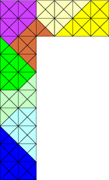
Decomposition	Reference map	Range
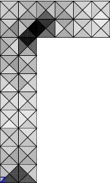
Iteration 1	Iteration 4	Iteration 5
	BDD solver
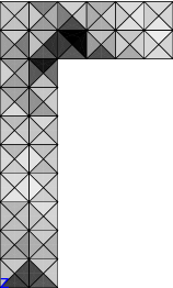
Iteration 1	Iteration 4	Iteration 5
	FETI solver

Figure 5: Maps of $\mathrm{e_{CR}^{ddm,E}}$ for $h=L/2$ and $N_{sd}=8$ at various iterations

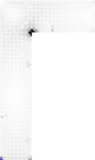
Decomposition	Reference map	Range
Iteration 1	Iteration 4	Iteration 5
	BDD solver
Iteration 1	Iteration 4	Iteration 5
	FETI solver

Figure 6: Maps of $\mathrm{e_{CR}^{ddm,E}}$ for $h=L/8$ and $N_{sd}=8$ at various iterations

7 Conclusions

In this paper, we presented a new approach to handle robust model verification based on constitutive relation error in a domain decomposition context.

The method relies on the construction of fields that are kinematically and statically admissible on the whole structure. We showed that a fully parallel construction is possible even when starting from fields which do not satisfy interface conditions. The construction is a three-step procedure: first displacement and traction nodal fields are built-up so that discrete admissibility conditions are satisfied, second continuous admissible traction fields are deduced, third these fields are used as input by any classical recovery procedure. The first step is implicitly done when good preconditioners are employed within the domain decomposition methods and the second step corresponds to the inversion of small and sparse “mass” matrices.

Our first results show that not only the estimation error does not suffer from the approximation that are made at the interface in order to achieve full parallelism, but that even roughly estimated interface fields enable to obtain a good estimation of the discretization error and correct maps of elementary contributions which are required by mesh adaptation procedures. Thus not only the computational cost are divided by the number of processors but the prior obtainment of the finite element solution can be accelerated since a coarse solution is sufficient (which corresponded to 3 to 5 times less iterations in our case).

Future studies will deal with parallel mesh adaptation.

\psfrag{a}{$1^{(1)}$}\psfrag{b}{$2^{(1)}$}\psfrag{c}{$3^{(1)}$}\psfrag{d}{$4^{(1)}$}\psfrag{e}{$5^{(1)}$}\psfrag{f}{$1^{(2)}$}\psfrag{g}{$2^{(2)}$}\psfrag{h}{$3^{(2)}$}\psfrag{i}{$4^{(2)}$}\psfrag{j}{$5^{(2)}$}\psfrag{k}{$1^{(3)}$}\psfrag{l}{$2^{(3)}$}\psfrag{m}{$3^{(3)}$}\psfrag{n}{$4^{(3)}$}\psfrag{ct}{$1_{b}^{(1)}$}\psfrag{dt}{$2_{b}^{(1)}$}\psfrag{et}{$3_{b}^{(1)}$}\psfrag{ht}{$1_{b}^{(2)}$}\psfrag{it}{$2_{b}^{(2)}$}\psfrag{jt}{$3_{b}^{(2)}$}\psfrag{kt}{$1_{b}^{(3)}$}\psfrag{lt}{$2_{b}^{(3)}$}\psfrag{mt}{$3_{b}^{(3)}$}\psfrag{o}{$1_{\Gamma}$}\psfrag{p}{$2_{\Gamma}$}\psfrag{q}{$3_{\Gamma}$}\psfrag{r}{$4_{\Gamma}$}\psfrag{s}{$\underline{1}_{\Gamma}$}\psfrag{t}{$\underline{2}_{\Gamma}$}\psfrag{u}{$\underline{3}_{\Gamma}$}\psfrag{v}{$\underline{4}_{\Gamma}$}\psfrag{w}{$\underline{5}_{\Gamma}$}\psfrag{x}{$\underline{6}_{\Gamma}$}\includegraphics[width=142.26378pt]{omegef2a.eps}

(a) Subdomains

\psfrag{a}{$1^{(1)}$}\psfrag{b}{$2^{(1)}$}\psfrag{c}{$3^{(1)}$}\psfrag{d}{$4^{(1)}$}\psfrag{e}{$5^{(1)}$}\psfrag{f}{$1^{(2)}$}\psfrag{g}{$2^{(2)}$}\psfrag{h}{$3^{(2)}$}\psfrag{i}{$4^{(2)}$}\psfrag{j}{$5^{(2)}$}\psfrag{k}{$1^{(3)}$}\psfrag{l}{$2^{(3)}$}\psfrag{m}{$3^{(3)}$}\psfrag{n}{$4^{(3)}$}\psfrag{ct}{$1_{b}^{(1)}$}\psfrag{dt}{$2_{b}^{(1)}$}\psfrag{et}{$3_{b}^{(1)}$}\psfrag{ht}{$1_{b}^{(2)}$}\psfrag{it}{$2_{b}^{(2)}$}\psfrag{jt}{$3_{b}^{(2)}$}\psfrag{kt}{$1_{b}^{(3)}$}\psfrag{lt}{$2_{b}^{(3)}$}\psfrag{mt}{$3_{b}^{(3)}$}\psfrag{o}{$1_{\Gamma}$}\psfrag{p}{$2_{\Gamma}$}\psfrag{q}{$3_{\Gamma}$}\psfrag{r}{$4_{\Gamma}$}\psfrag{s}{$\underline{1}_{\Gamma}$}\psfrag{t}{$\underline{2}_{\Gamma}$}\psfrag{u}{$\underline{3}_{\Gamma}$}\psfrag{v}{$\underline{4}_{\Gamma}$}\psfrag{w}{$\underline{5}_{\Gamma}$}\psfrag{x}{$\underline{6}_{\Gamma}$}\includegraphics[width=142.26378pt]{omegef2b.eps}

(b) Local interface

\psfrag{a}{$1^{(1)}$}\psfrag{b}{$2^{(1)}$}\psfrag{c}{$3^{(1)}$}\psfrag{d}{$4^{(1)}$}\psfrag{e}{$5^{(1)}$}\psfrag{f}{$1^{(2)}$}\psfrag{g}{$2^{(2)}$}\psfrag{h}{$3^{(2)}$}\psfrag{i}{$4^{(2)}$}\psfrag{j}{$5^{(2)}$}\psfrag{k}{$1^{(3)}$}\psfrag{l}{$2^{(3)}$}\psfrag{m}{$3^{(3)}$}\psfrag{n}{$4^{(3)}$}\psfrag{ct}{$1_{b}^{(1)}$}\psfrag{dt}{$2_{b}^{(1)}$}\psfrag{et}{$3_{b}^{(1)}$}\psfrag{ht}{$1_{b}^{(2)}$}\psfrag{it}{$2_{b}^{(2)}$}\psfrag{jt}{$3_{b}^{(2)}$}\psfrag{kt}{$1_{b}^{(3)}$}\psfrag{lt}{$2_{b}^{(3)}$}\psfrag{mt}{$3_{b}^{(3)}$}\psfrag{o}{$1_{\Gamma}$}\psfrag{p}{$2_{\Gamma}$}\psfrag{q}{$3_{\Gamma}$}\psfrag{r}{$4_{\Gamma}$}\psfrag{s}{$\underline{1}_{\Gamma}$}\psfrag{t}{$\underline{2}_{\Gamma}$}\psfrag{u}{$\underline{3}_{\Gamma}$}\psfrag{v}{$\underline{4}_{\Gamma}$}\psfrag{w}{$\underline{5}_{\Gamma}$}\psfrag{x}{$\underline{6}_{\Gamma}$}\includegraphics[width=142.26378pt]{omegef2c.eps}

(c) Primal interface

\psfrag{a}{$1^{(1)}$}\psfrag{b}{$2^{(1)}$}\psfrag{c}{$3^{(1)}$}\psfrag{d}{$4^{(1)}$}\psfrag{e}{$5^{(1)}$}\psfrag{f}{$1^{(2)}$}\psfrag{g}{$2^{(2)}$}\psfrag{h}{$3^{(2)}$}\psfrag{i}{$4^{(2)}$}\psfrag{j}{$5^{(2)}$}\psfrag{k}{$1^{(3)}$}\psfrag{l}{$2^{(3)}$}\psfrag{m}{$3^{(3)}$}\psfrag{n}{$4^{(3)}$}\psfrag{ct}{$1_{b}^{(1)}$}\psfrag{dt}{$2_{b}^{(1)}$}\psfrag{et}{$3_{b}^{(1)}$}\psfrag{ht}{$1_{b}^{(2)}$}\psfrag{it}{$2_{b}^{(2)}$}\psfrag{jt}{$3_{b}^{(2)}$}\psfrag{kt}{$1_{b}^{(3)}$}\psfrag{lt}{$2_{b}^{(3)}$}\psfrag{mt}{$3_{b}^{(3)}$}\psfrag{o}{$1_{\Gamma}$}\psfrag{p}{$2_{\Gamma}$}\psfrag{q}{$3_{\Gamma}$}\psfrag{r}{$4_{\Gamma}$}\psfrag{s}{$\underline{1}_{\Gamma}$}\psfrag{t}{$\underline{2}_{\Gamma}$}\psfrag{u}{$\underline{3}_{\Gamma}$}\psfrag{v}{$\underline{4}_{\Gamma}$}\psfrag{w}{$\underline{5}_{\Gamma}$}\psfrag{x}{$\underline{6}_{\Gamma}$}\includegraphics[width=142.26378pt]{omegef2d.eps}

(d) Dual interface

$$\begin{array}[]{rclrclrcl}\mathbf{t}^{(1)}&=&\begin{pmatrix}0&0&1&0&0\\ 0&0&0&1&0\\ 0&0&0&0&1\end{pmatrix},&\mathbf{t}^{(2)}&=&\begin{pmatrix}0&0&1&0&0\\ 0&0&0&1&0\\ 0&0&0&0&1\end{pmatrix},&\mathbf{t}^{(3)}&=&\begin{pmatrix}1&0&0&0\\ 0&1&0&0\\ 0&0&1&0\end{pmatrix}\\ \mathbf{A}^{(1)}&=&\begin{pmatrix}0&0&0\\ 0&1&0\\ 1&0&0\\ 0&0&1\end{pmatrix},&\mathbf{A}^{(2)}&=&\begin{pmatrix}1&0&0\\ 0&0&1\\ 0&0&0\\ 0&1&0\end{pmatrix},&\mathbf{A}^{(3)}&=&\begin{pmatrix}0&0&1\\ 0&0&0\\ 1&0&0\\ 0&1&0\end{pmatrix}\\ \mathbf{\underline{A}}^{(1)}&=&\begin{pmatrix}0&0&0\\ 0&1&0\\ 1&0&0\\ 0&0&0\\ 0&0&1\\ 0&0&1\end{pmatrix},&\mathbf{\underline{A}}^{(2)}&=&\begin{pmatrix}1&0&0\\ 0&0&-1\\ 0&0&0\\ 0&1&0\\ 0&-1&0\\ 0&0&0\end{pmatrix},&\mathbf{\underline{A}}^{(3)}&=&\begin{pmatrix}0&0&-1\\ 0&0&0\\ -1&0&0\\ 0&-1&0\\ 0&0&0\\ 0&-1&0\end{pmatrix}\end{array}$$

Figure 7: Local numberings, interface numberings, trace and assembly operators

References

- [1] I. Babuska, W. Rheinboldt, Error estimates for adaptative finite element computation, SIAM J. Num. Anal. 15 (4) (1978) 736–754.
- [2] O. Zienkiewicz, J. Zhu, A simple error estimate and adaptative procedure for practical engineering analysis, Int. J. for Num. Meth. in Engrg. 24 (1987) 337–357.
- [3] P. Ladevèze, Comparaison de modèles de milieux continus, Thèse de doctorat d’état, Université Pierre et Marie Curie, 75005 Paris, France, 1975.
- [4] P. Ladevèze, J. Pelle, Mastering calculations in linear and nonlinear mechanics, Springer, 2004.
- [5] C. Farhat, F. X. Roux, Implicit parallel processing in structural mechanics, Computational Mechanics Advances 2 (1) (1994) 1–124, north-Holland.
- [6] J. Mandel, Balancing domain decomposition, Comm. Appl. Num. Meth. Engrg. 9 (1993) 233–241.
- [7] P. Gosselet, C. Rey, Non-overlapping domain decomposition methods in structural mechanics, Archives of computational methods in engineering 13 (4) (2007) 515–572.
- [8] P. Ladevèze, D. Leguillon, Error estimate procedure in the finite element method and application, Siam. J. on Num. Analysis 20 (3) (1983) 485–509.
- [9] P. Ladevèze, P. Rougeot, New advances on a posteriori error on constitutive relation in f.e. analysis, Comp. Meth. Appl. Mech. Eng. 150 (1-4) (1997) 239–249.
- [10] N. Parés, P. Díez, A. Huerta, Subdomain-based flux-free a posteriori error estimators, Comp. Meth. Appl. Mech. Eng. 195 (4-6) (2006) 297–323.
- [11] L. Gallimard, A constitutive relation error estimator based on traction-free recovery of the equilibrated stress, Int. J. for Num. Meth. in Engrg. 78 (4) (2009) 460–482.
- [12] J. P. M. de Almeida, E. A. W. Maunder, Recovery of equilibrium on star patches using a partition of unity technique, Int. J. for Num. Meth. in Engrg. 79 (12) (2009) 1493–1516.
- [13] P. Ladevèze, L. Chamoin, E. Florentin, A new non-intrusive technique for the construction of admissible stress fields in model verification, Comp. Meth. Appl. Mech. Eng. 199 (9-12) (2010) 766–777.
- [14] P. Beckers, E. Dufeu, 3-d error estimation and mesh adaptation using improved r.e.p. method, Stud. Appl. Mech. 47 (1998) 413–426.
- [15] I. Babuska, T. Strouboulis, C. Upadhyay, S. Gangaraj, K. Copps, Validation of a posteriori error estimators by numerical approach, Int. J. Num. Meth. Engng. 37 (1994) 1073–1123.
- [16] J. Mandel, Balancing domain decomposition, Comm. Appl. Num. Meth. Engrg. 9 (1993) 233–241.
- [17] P. L. Tallec, Domain-decomposition methods in computational mechanics, Computational Mechanics Advances 1 (2) (1994) 121–220, north-Holland.
- [18] D. Rixen, C. Farhat, A simple and efficient extension of a class of substructure based preconditioners to heterogeneous structural mechanics problems, Int. J. Num. Meth. Eng. 44 (4) (1999) 489–516.
- [19] A. Klawonn, O. Widlund, FETI and Neumann-Neumann iterative substructuring methods: connections and new results, Comm. pure and appl. math. LIV (2001) 0057–0090.
- [20] P. Gosselet, C. Rey, P. Dasset, F. Léné, A domain decomposition method for quasi incompressible formulations with discontinuous pressure field, Revue européenne des élements finis 11 (2002) 363–377.
- [21] P. Gosselet, C. Rey, D. Rixen, On the initial estimate of interface forces in FETI methods, Comp. meth. appl. mech. engrg. 192 (2003) 2749–2764.
- [22] L. Chamoin, P. Ladeveze, A non-intrusive method for the calculation of strict and efficient bounds of calculated outputs of interest in linear viscoelasticity problems, Comp. Meth. Appl. Mech. Eng. 197 (9-12) (2008) 994–1014.
- [23] Northwest Numerics, Z-set user manual (2001).