Composite fermion state of spin-orbit coupled bosons

Abstract

We consider spinor Bose gas with the isotropic Rashba spin-orbit coupling in 2D. We argue that at low density its groundstate is a composite fermion state with a Chern-Simons gauge field and filling factor one. The chemical potential of such a state scales with the density as $\mu\propto n^{3/2}$. This is a lower energy per particle than $\mu\propto n$ for the earlier suggested groundstate candidates: a condensate with broken time-reversal symmetry and a spin density wave state.

I Introduction

Precise control over interactions of ultracold atoms with laser fields opened an opportunity of fabricating synthetic non-Abelian gauge fieldsLin-2008 ; Lin-2009 ; synthetic and spin-orbit (SO) couplingsLin-2011 ; zhang-exp of both RashbaRashba and DresselhausDresselhaus type. In analogy with previously known vector condensatesstenger ; ho ; law ; ashhab ; svist , an important tool for synthesizing such systems is the controlled Raman coupling between oriented sequence of initially degenerate hyperfine states of ⁸⁷Rb. Interactions of spatially varying laser field with hyperfine atomic levels effectively produces synthetic non-Abelian gauge fields,Jaksch ; Ruseckas ; Osterloh ; Zhu originating from the Berry phase, and SO couplingLin-2011 ; zhang-exp ; tudor ; SAG ; dalibard ; Campbell-2011 ; dalibard2 ; 3D of momentum to the internal isospin degrees of freedom. Bosons with SO coupling, discussed and studied in the context of cold-atom physics in Ref. [SAG, ], were realized very recently by Spielman’s group at NISTLin-2011 . Depending on the particular experimental scheme, i.e. the choice of atomic states and a sequence of optically induced transitions between them, one may in principle realize various SO Hamiltonians for the projected low-energy states. Low energy properties of such SO bosonic systems have been discussed in Refs. [SAG, ; zhai, ; Wu, ; radic, ; ho11, ; Lamacraft, ; zhai2, ; yongping, ; DasSarma, ; ozawa, ; ozawa2, ; pitaevskii, ].

While fermions with SO coupling were extensively studied over the last decades, see e.g. Refs. [kato, ; hasan, ; nagaosa, ; zutic, ] for reviews, relatively little is known about SO bosons. Yet, they offer a number of fundamental problems which, in some respects, are more challenging than their fermionic counterparts. Indeed, in many instances SO coupling leads to single-particle dispersion relations which exhibit multiple minima or even degenerate manifold of minimal energy states. Fermionic many-body systems form a unique Fermi sea state on top of such dispersion relation. On the other hand, bosons tend to occupy the lowest energy states and thus face macroscopic degeneracy of their non-interacting groundstate. It is entirely the effect of collisions (i.e. boson-boson interactions) which lifts this degeneracy and selects a true many-body groundstate.

In this respect the problem is somewhat similar to fractional quantum Hall effect (FQHE). There the fermionic kinetic energy is degenerate due to Landau quantization and the nature of the groundstate is determined by the interactions. One of the most remarkable concepts, which emerged in FQHE studies, is that of composite particlesJain ; lopez ; Halperin ; SDS ; heinonen ; jbook . For example, FQHE states with filling fractions $\nu=p/(2p+1)$, where $p=1,2\ldots$, were understood as integer $\nu=p$ quantum Hall states of composite fermion particles. The latter are obtained by binding the original fermions with flux tubes carrying exactly two flux quanta. Technically such a binding is achieved by assigning Chern-Simons (CS) phase factor to the many-body wavefunction of composite particles.

The goal of this paper is to show that a very similar transformation plays a major role in understanding of the groundstate of 2D bosons with Rashba SO coupling. We argue here that their groundstate wavefunction may be approximated by that of the Fermi gas at integer filling factor $\nu=1$, dressed by the Chern-Simons phase with one flux quantum attached to every fermion. Such phase factor transforms the integer quantum Hall fermionic wavefunction into a bosonic one. Fermionization of the bosonic system allows the latter to minimize its interaction energy. This is due to the fact that fermions with the same spin can’t be at the same spatial point and thus cannot interact through a short-range s-wave interaction. (Consequently the amplitude for two fermions with almost parallel spins to be at the same point is small as the angle between their spins.) As the result the interaction energy per particle in a Fermi sea is smaller than in a Bose-condensate of the same density. For low enough density such reduction of the interaction energy wins over the associate increase of the kinetic energy.

A very similar physics is behind the so-called Tonks-Girardeau limit of spinless 1D Bose gasLiebLiniger ; tonks ; girardeau . At a small density (which in 1D is the same as strong interactions) the bosonic wavefunction approaches symmetrized wavefunction of non-interacting Fermi gas. If spin degree of freedom is present in 1D, the groundstate is known to be fully spin-polarizedlieb ; yang ; gaudin again leading to the Tonks-Girardeau construction in low density limit. We thus notice that 2D Rashba bosons share features of both 2D quantum Hall systems as well as 1D Bose gases. The deep connection with the latter is due to the fact that single-particle density of states for particles with Rashba SO coupling behaves as $\epsilon^{-1/2}$ at small energy. This is typical for 1D systems, making particles with Rashba SO coupling “1D-like”, irrespective of their actual spatial dimensionality.

Technically blending FQHE and Tonks-Girardeau ideas with Rashba SO coupling presents one with a number of challenges. Indeed, the standard way of introducing Chern-Simons transformationJain ; Halperin essentially relies on the spinless nature of particles. Here we suggest a way to generalize it for spinor particles with strong SO coupling. It achieves the goal of fermionization of bosons, but fails to eliminate completely the interactions between the composite spinless fermions. Still the fermionic interaction energy can be parametrically smaller than the bosonic one. The crucial observation here is that the residual fermion-fermion interactions appear to be proportional to the angle between momenta of two scattering particles. Therefore, confining the Fermi sea of composite fermions to a small fraction of the momentum space, allows one to lower their interaction energy. Similar ideas were recently put forward by Berg, Rudner and Kivelson (BRK)berg in the context of Fermi gas with Rashba SO coupling. They called the resulting time-reversal symmetry broken state a nematic. Here we adopt their construction for the composite fermions.

The paper is organized as follows: in section II we introduce Rashba SO coupling on a single-particle level. We also discuss earlier mean-field theories for bosonic many-body groundstates along with BRK nematic state for many-body fermionic system. In section III we introduce fermionization of spinor bosons and evaluate the energy of the resulting composite fermion state. In section IV we discuss the results: present an emerging groundstate phase diagram of Rashba bosons, list possible experimental consequences and generalizations of our approach. Some technical details of the calculations are relegated to the Appendix.

II Rashba spin-orbit coupling

II.1 Single particle spectrum

The single-particle Hamiltonian with the Rashba spin-orbit coupling in two dimensions takes the form

$$H_{0}=-\frac{{\bm{\nabla}}_{\bf r}^{2}}{2m}+iv\hat{\bf z}\cdot[\bm{\sigma}\times{\bm{\nabla}_{\bf r}}]\,,$$ (1)

where $v$ is spin-orbit coupling constant having dimensionality of velocity, ${\bm{\nabla}}_{\bf r}=(\partial_{x},\partial_{y})$ and $\bm{\sigma}=(\sigma_{x},\sigma_{y})$ is vector of Pauli matrices acting on two component spinor $\psi(\bf r)=\left(\psi(\bf r,\uparrow),\psi(\bf{r},\downarrow)\right)$. In 2D the Rashba term in Eq. (1) may be transformed to another form $iv\bm{\sigma}\cdot{\bm{\nabla}_{r}}$ by $\pi/2$ rotation in the spin space.

In addition to translational and rotational symmetries the Hamiltonian $H_{0}$ commutes with the two discrete $Z_{2}$ symmetry operations: time-reversal $\hat{T}$ and 2D parity $\hat{P}$. They may be defined in the following way

$$\hat{T}\left(\begin{array}[]{r}\psi(\bf r,\uparrow)\\ \psi(\bf r,\downarrow)\end{array}\right)=\left(\begin{array}[]{r}\bar{\psi}(\bf r,\downarrow)\\ -\bar{\psi}(\bf{r},\uparrow)\end{array}\right)$$ (2)

and

$$\hat{P}\left(\begin{array}[]{r}\psi(z,\uparrow)\\ \psi(z,\downarrow)\end{array}\right)=\left(\begin{array}[]{r}-i\psi(\bar{z},\downarrow)\\ i\psi(\bar{z},\uparrow)\end{array}\right),$$ (3)

where bar stands for complex conjugated and we introduced the complex 2D coordinate as $z=x+iy$. Notice that the parity operation in 2D is defined as $y\to-y$ and $x\to x$ and $\sigma_{y}$ multiplication. Indeed, reflection of both coordinates $x$ and $y$ is equivalent to $\pi$ rotation. Of course, one could as well define parity as $x$ reflection and $\sigma_{x}$ multiplication. It is equivalent to the $P$ operation (3) combined with the $\pi$ rotation.

Diagonalization of the Hamiltonian (1) yields the following single-particle spectrum:

$$\varepsilon_{{\bf k},\gamma}=\frac{{k}^{2}}{2m}+\gamma vk.$$ (4)

Here index $\gamma=\pm 1$ labels the two brunches of the spectrum depicted in Fig. 1. The corresponding eigenfunctions are plane waves in coordinate space multiplying coordinate-independent spinor, whose form depends, however, on the momentum ${\bf k}$ as

$$\psi_{{\bf k},\gamma}({\bf r},s)=\frac{1}{\sqrt{2V}}\left(\begin{array}[]{c}-i\gamma\,e^{-i\text{arg}({\bf k})}\\ 1\\ \end{array}\right)_{s}\,e^{i{\bf k}{\bf r}}.$$ (7)

where $\text{arg}({\bf k})$ is the angle between the momentum vector ${\bf k}$ and the $k_{x}$-axis, $V$ is the system’s volume. The spin is directed in the $x-y$ plane and is rotated relative to the momentum direction by $\gamma\pi/2$. Hereafter we consider SO energy scale $\epsilon_{0}=mv^{2}/2$ as the largest energy in the problem. One thus expects the groundstate of an interacting system to be confined to the part of the Hilbert space projected on the lower branch $\gamma=-1$. Clearly the two spin components of all such states are connected by the following unitary transformation $\psi_{{\bf k},-}({\bf r},\uparrow)=ie^{-i\arg({\bf k})}\psi_{{\bf k},-}({\bf r},\downarrow)$. For a generic wavefunction belonging to the lower branch the relation between its up and down components acquires the form

$$\psi({\bf r},\uparrow) = \int d{\bf r}^{\prime}\,{\cal R}({\bf r}-{\bf r}^{\prime})\,\psi({\bf r}^{\prime},\downarrow),$$ (8)

where the spin-raising kernel

$${\cal R}({\bf r}-{\bf r}^{\prime}) = -\frac{1}{2\pi}\,\frac{e^{-i\mathrm{arg}({\bf r}-{\bf r}^{\prime})}}{({\bf r}-{\bf r}^{\prime})^{2}}$$ (9)

is the Fourier transform of $ie^{-i\arg({\bf k})}$. Importantly, the ${\cal R}$-operator in real space has the unitarity property, $\int d{\bf r}\bar{\cal R}({\bf r}-{\bf r}_{1}){\cal R}({\bf r}-{\bf r}_{2})=\delta({\bf r}_{1}-{\bf r}_{2})$, which is the direct consequence of the unitarity of the spin-rising transformation in the momentum space representation.

The most notable feature of the dispersion relation (4) is that its groundstate is degenerate along the circle in the momentum space $k=k_{0}=mv$. As a result the many-body groundstate of $N$ non-interacting bosons is highly degenerate (not so for fermions, though). Indeed, any occupation of the states along the groundstate circle $k=k_{0}$ yields exactly the same kinetic energy $-Nk_{0}^{2}/2m$. Hereafter we shall measure the energy from that value, taking it for the origin of the energy axis. It is therefore only the interactions, which may break the degeneracy and select a true groundstate. The situation is similar to a partially filled Landau level in the context of FQHE. There too the kinetic energy is fully degenerate and the groundstate is solely determined by the interparticle interactions.

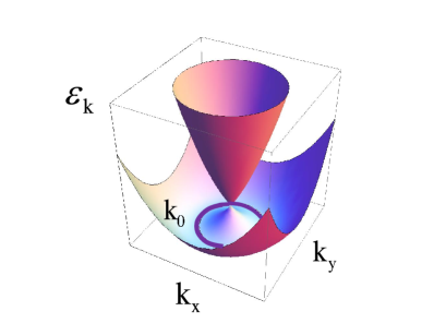
Figure 1: (Color online) Dispersion relation (4) of particles with Rashba SO coupling. The degenerate groundstate ${\bf k}=k_{0}=mv$ is shown by full circle.

II.2 Bosons with Rashba dispersion

Let us consider $N$ particles with the $s$-wave short-range interactions of the form

$$H_{\mathrm{int}}=\frac{1}{2m}\sum_{i,j}^{N}\delta({\bf r}_{i}-{\bf r}_{j})\big{[}g_{0}+g_{2}\sigma_{z}^{(i)}\sigma_{z}^{(j)}\big{]},$$ (10)

where $g_{0}$ is the spin-isotropic dimensionless interaction constant, while $g_{2}$ is the spin-anisotropic interaction constant.

One can now evaluate interaction energy of certain simple $N$-body Bose states. One such state is a Bose-Einstein condensate in a single state belonging to a degenerate manifold of the single-particle ground states, i.e. a state with momentum ${\bf k}$, such that $k=k_{0}$ and $\gamma=-1$,

$$\Psi^{(0)}_{B}=\prod_{i=1}^{N}\psi_{{\bf k},-}({\bf r}_{i},s_{i})\,.$$ (11)

This wavefunction is obviously symmetric with respect to the permutation of any two pairs $({\bf r}_{i},s_{i})\leftrightarrow({\bf r}_{j},s_{j})$. Such a state is not symmetric under time-reversal transformation $\hat{T}$, Eq. (2), because of unequal population of ${\bf k}$ and $-{\bf k}$ states. We shall call it thus time-reversal symmetry broken (TRSB) state. Note that this state does not break the parity $\hat{P}$, Eq. (3). To see it most clearly one may choose momentum ${\bf k}$ direction to be along the $x$-axis. Calculating the expectation value of the interaction energy (10) over TRSB state, one finds

$$E^{(0)}_{\mathrm{int}}=\frac{N^{2}}{2mV}\,g_{0}\,.$$ (12)

Since the kinetic energy in the state (11) is zero, the interaction energy (12) coincides with the total one.

One may consider now a Bose condensate built on a coherent superposition of say two states ${\bf k}_{1}$ and ${\bf k}_{2}$ both belonging to the degenerate manifold $k=k_{0}$:

$$\Psi^{\mathrm{(\phi)}}_{B}=\prod_{i=1}^{N}\frac{1}{\sqrt{2}}\left[\psi_{{\bf k}_{1},-}({\bf r}_{i},s_{i})+\psi_{{\bf k}_{2},-}({\bf r}_{i},s_{i})\right]\,.$$ (13)

The corresponding interaction (and thus total) energy is found to be

$$E^{(\phi)}_{\mathrm{int}}=\frac{N^{2}}{2mV}\,\left[g_{0}+{g_{0}\over 2}\cos^{2}{\phi\over 2}+{g_{2}\over 2}\sin^{2}{\phi\over 2}\right]\,,$$ (14)

where $\phi=\text{arg}({\bf k}_{1})-\text{arg}({\bf k}_{2})$ is the angle between the two states of the degenerate manifold. It is clear that, provided the spin-isotropic interaction is repulsive $g_{0}>0$, the only way the state (13) may be energetically more favorable than the state (11) is if $g_{2}<0$. In the latter case the most favorable choice of the two states corresponds to $\phi=\pi$, i.e. ${\bf k}_{2}=-{\bf k}_{1}$, with the interaction energy $E^{(\pi)}_{\mathrm{int}}=(N^{2}/2mV)\,\left[g_{0}+g_{2}/2\right]$. Such a state represents a spin density wave (SDW) with a uniform total density and the two spin components oscillating harmonically out of phase. It is symmetric with respect to both time-reversal and parity symmetries, Eqs. (2), (3), but breaks the rotational symmetry. In either of these states the kinetic energy is zero.

It was conjectured zhai ; Wu that TRSB $\Psi^{(0)}_{B}$, (11), and the SDW state $\Psi^{(\pi)}_{B}$, (13), are the many-body groundstates of the Rasba interacting bosons for $g_{2}>0$ and $g_{2}<0$ correspondingly. It was later suggested Lamacraft that the transition between TRSB and SDW states is shifted towards positive $g_{2}$ due to a ceratin admixture of coherently occupied BCS-like pairs of ${\bf k}$ and $-{\bf k}$ states. We notice that for both of these states the chemical potential scales linearly with the density $n=N/V$,

$$\mu_{B}=\partial E_{\mathrm{int}}/\partial N\propto n\,.$$ (15)

It is instructive to compare this scaling of the bosonic chemical potential with the corresponding fermionic one.

II.3 Fermions with Rashba dispersion

Unlike bosons, the non-interacting Fermi gas exhibits the unique ground-state. It is given by the rotationally symmetric Fermi sea with the Fermi surface consisting of two concentric circles with the radii $k_{F\pm}=k_{0}\pm 2\pi n/k_{0}$, hereafter the small density $n\ll k_{0}^{2}$ is assumed. The corresponding Fermi energy measured from the bottom of the spectrum is

$$\mu_{F}^{(0)}=\frac{(\pi n)^{2}}{2mk_{0}^{2}}\,.$$ (16)

Notice the fact that $\mu_{F}^{(0)}\propto n^{2}$, which is usually the feature of 1D Fermi gas. Here it happens because the single-particle density of states exhibits 1D-like behavior $\nu(\epsilon)\propto\epsilon^{-1/2}$ close to the bottom of the Rashba circle. The interesting observation is that at small enough density $n\lesssim g_{0}k_{0}^{2}$ the chemical potential of interacting bosons appears to be bigger than that of the free Fermi gas with the same dispersion relation (4). Before making conclusions from this observation one needs to consider the interaction energy (10) of the Fermi sea state.

Spinless (or fully spin-polarized) fermions do not interact through short-range interactions. In our case the particles have spin, which is locked to their orbital momenta. As a result the symmetric Fermi sea, described above, contains all spin directions in x-y plane with equal weights. Since two fermions with opposite spins interact through the short range interaction (10), one expects the average interaction energy of the symmetric Fermi sea to be of the same order as bosonic one $\propto g_{0}N^{2}/mV$ and thus $\mu_{F}\propto n$ similarly to the bosonic condensates. It was recently noticed by Berg, Rudner and Kivelson berg that low density Rashba fermions may have parametrically lower groundstate energy if they form a nematic state.

To motivate the idea, let us consider two-fermion state as a Slater determinant built on single particle states (7) with momenta ${\bf k}_{1,2}$ close to the Rashba circle $\Psi_{F}=[\psi_{{\bf k}_{1},-}({\bf r}_{1},s_{1})\psi_{{\bf k}_{2},-}({\bf r}_{2},s_{2})-\psi_{{\bf k}_{1},-}({\bf r}_{2},s_{2})\psi_{{\bf k}_{2},-}({\bf r}_{1},s_{1})]/\sqrt{2}$. The interaction energy (10) of such state is given by $E_{\mathrm{int}}=\sin^{2}(\phi/2)(g_{0}+g_{2})/2m$, where $\phi=\mathrm{arg}({\bf k}_{1})-\mathrm{arg}({\bf k}_{2})$. Therefore the interaction energy between fermions tends to zero if $\mathrm{arg}({\bf k}_{1})\to\mathrm{arg}({\bf k}_{2})$, essentially because the spins are aligned in this limit and fermions with the same spin can not interact through the short-range interaction potential. The BRK nematic state takes advantage of this observation.

To describe such a state qualitatively let us imagine that the many-body fermionic state $\Psi_{F}$ is constructed as a Slater determinant of states with the angular directions confined to the angular segment of the momentum (and spin) space of size $\Theta\ll 2\pi$ and momenta close to the spin-orbit circle $||{\bf k}_{j}|-k_{0}|<k_{F}^{(\Theta)}$, Fig. 2. The corresponding Fermi momentum is found from the condition $2k_{F}^{(\Theta)}k_{0}\Theta=(2\pi)^{2}n$. As a result the corresponding kinetic energy per particle $E_{\mathrm{kin}}/N\propto[k_{F}^{(\Theta)}]^{2}/m\propto n^{2}/(m\Theta^{2}k_{0}^{2})$. On the other hand, the interaction energy per particle is $E_{\mathrm{int}}/N\propto(g_{0}+g_{2})n\Theta^{2}/m$, with the factor $\Theta^{2}$ originating from $\sin^{2}(\phi/2)\sim\Theta^{2}$. One can now minimize the sum of kinetic and interaction energy over $\Theta$ to find $\Theta\propto[n/k_{0}^{2}(g_{0}+g_{2})]^{1/4}$, which is indeed small as long as

$$n\ll n_{0}=k_{0}^{2}(g_{0}+g_{2})\,.$$ (17)

With this $\Theta$ the chemical potential of short-range interacting fermions with Rashba spin-orbit coupling is found to be $\mu_{F}\propto n^{3/2}\sqrt{g_{0}+g_{2}}/mk_{0}$, which is the result of BRKberg . In the small density limit (17) the latter is bigger than that of non-interacting Rashba fermions (16), but is advantageous over bosonic TRSB and SDW states (15): $\mu_{F}^{(0)}<\mu_{F}<\mu_{B}$. Notice also the non-analytic dependence of $\mu_{F}$ on the interaction strength, indicating the non-perturbative nature of this result. We show in Section III.4 that the composite fermion nematic state may be described quantitatively within Hartree-Fock self-consistent mean-field treatment, Fig. 2.

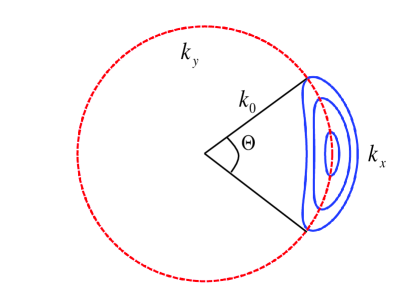
Figure 2: (Color online) Hartree-Fock Fermi surfaces of BRK nematic states with three different densities. The absolute value of the momenta are restricted to the vicinity of the Rashba circle ${\bf k}=k_{0}$, while their angular directions are restricted to the angle $\Theta\propto[n/k_{0}^{2}(g_{0}+g_{2})]^{1/4}$.

II.4 Can bosons be fermions?

We have arrived thus to the conclusion that at low density (17) the chemical potential and groundstate energy of fermionic many-body system is smaller than the corresponding bosonic one. The similar situation seemingly happens in a 1D system of spinless particles with short range interaction potential $(g_{0}/m)\delta(x_{i}-x_{j})$. There too the mean-field treatment of bosons suggests that $\mu_{B}\sim g_{0}n$. On the the other hand, spinless fermions (which are not affected by short-range interactions due to the Pauli principle) exhibit $\mu_{F}\sim n^{2}$. It thus seems that at a small enough density the fermionic groundstate energy is smaller than the bosonic one. The actual situation is, of course, very differentLiebLiniger . At small density bosonic many-body groundstate wavefunction $\Psi_{B}$ approaches the symmetrized fermionic one

$$\Psi_{B}(x_{1},\ldots,x_{N})=\prod_{i,j}^{N}\mbox{sign}(x_{i}-x_{j})\Psi_{F}(x_{1},\ldots,x_{N})\,,$$ (18)

where $\Psi_{F}$ is the fermionic Slater determinant occupying a finite portion of the momentum space $-\pi n\leq k\leq\pi n$. It is important to notice that, although $\mbox{sign}(x_{i}-x_{j})$ is undefined at $x_{i}=x_{j}$, the fermionic part cancels at all such points making $\Psi_{B}(x_{1},\ldots,x_{N})$ well-defined in the entire space. Due to the same observation there is no interaction energy cost for the short-range repulsion. The corresponding kinetic energy per particle $\propto(\pi n)^{2}/2m$ is small in the low density limit. This is the so-called Tonks-Girardeau limit tonks ; girardeau ; yang , where bosons redress themselves as fermions. This allows them to take advantage of the wavefunction, which is nullified at all points where any two particles approach each other. As a result they avoid paying short-range interaction energy cost, while corresponding kinetic energy cost appears to be worth the bargain at low density. The corresponding 1D equations of state are depicted in Fig. 3.

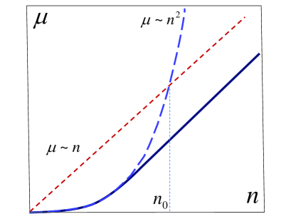
Figure 3: (Color online) Equations of state $\mu(n)$ of 1D quantum gases with short-range interactions: spinless Fermi gas (long-dashed); mean-field approximation for Bose gas (dashed); exact resultLiebLiniger for bosons (full). Notice that bosonic groundstate energy $E=\int\mu dn$ is always smaller than the fermionic one, although the mean-field treatment suggests otherwise for $n\lesssim n_{0}=g_{0}$.

It is thus tempting to speculate that our spinfull 2D system may benefit from a similar construction. Namely, at low density bosons may want to redress themselves as fermions to take advantage of their lower interaction energy. The blueprints of the boson-fermion correspondence in 2D are provided by FQHE studies Jain ; Halperin , where the correspondence is achieved by ascribing Chern-Simons phase factor to many-body wavefunctions. Such factor takes care of the proper symmetry of wavefunctions. It comes with the price however: the gauge magnetic field which has a form of delta-functional flux tubes attached to every particle. It is believed that (under proper conditions) this magnetic field may be substituted by a uniform one, making the problem analytically tractable. In the next section we develop a similar strategy for the chiral spinfull boson-fermion correspondence.

III Composite fermion state

III.1 Naïve fermionization attempt

Our goal is to construct a variational groundstate for Rashba bosons based on the composite fermion idea. We argue here that in the small density limit such a state, inspired by the Tonks-Girardeau limit (18), is advantageous over both TRSB (11) and SDW (13) bosonic states. The two main differences with the Tonks-Girardeau case are: (a) the 2D nature of our problem and (b) the spinfull nature of the particles. It is still tempting to straightforwardly generalize Eq. (18) to the 2D spinfull case by taking the variational ground state of the Bose gas in the following form:

$$\Psi_{B}({\bf r}_{1},s_{1},\cdots{\bf r}_{N},s_{N})$$ (19)

$$=\prod_{i<j}e^{i\arg({\bf r}_{i}-{\bf r}_{j})}\Psi_{F}({\bf r}_{1},s_{1},\cdots{\bf r}_{N},s_{N}),$$

where $\Psi_{F}({\bf r}_{1},s_{1},\cdots{\bf r}_{N},s_{N})$ is an N-particle fermionic wavefunction. The Chern-Simons phase $e^{i\arg({\bf r}_{i}-{\bf r}_{j})}={(z_{i}-z_{j})}/{|z_{i}-z_{j}|}$, with $z_{j}$ labeling complex spatial coordinates, $z_{j}=x_{j}+iy_{j}$, is antisymmetric with respect to exchange of any two coordinates. As a result, many-body wavefunction, $\Psi_{B}({\bf r}_{1},s_{1},\cdots{\bf r}_{N},s_{N})$, is symmetric under permutation of pairs ${\bf r}_{i},s_{i}$ and ${\bf r}_{j},s_{j}$ of coordinates and spins, $s_{i}=\uparrow,\downarrow$, if the fermionic wave function, $\Psi_{F}({\bf r}_{1},s_{1},\cdots{\bf r}_{N},s_{N})$, is antisymmetric with respect to the same permutations. One way of writing the latter is to take it as $N\times N$ Slater determinant of e.g. single-particle spinor wave functions, $\psi_{{\bf k}_{j},-}({\bf r}_{i},s_{i})$, Eq. (7), where $i,j=1,2,\ldots,N$.

While being probably the most straightforward way of guessing a spinfull composite fermion state, Eq. (19) has a number of fatal drawbacks. First, one might naïvely expect that similarly to Eq. (18), this ansatz maps the interacting bosonic system onto a system of non-interacting fermions. A closer look shows that this is not the case. Indeed, although the Slater determinant implies that the fermionic wave function has zeros at coinciding spatial points and spins, however for coinciding points and different spins the wavefunction is not nullified. As a result the composite fermions with opposite spins still do interact, despite the short-range nature of the interaction potential.

Even more serious problem with the trial wavefunction (19) is that it is not well-defined for coinciding points and opposite spins. This is due to the fact that the Chern-Simons phase is singular at coinciding points, while the fermionic part $\Psi_{F}$ is not vanishing if spins are opposite. This ambiguity leads to logarithmic divergent contributions to the average kinetic energy of the state (19). Indeed, consider the part of the kinetic energy $(2m)^{-1}\int d{\bf r_{i}}|\nabla_{{\bf r}_{i}}\Psi_{B}|^{2}$, where the gradient operators act on the Chern-Simons phases. This leads to the kinetic energy contribution of the form

$$\frac{1}{2m}\!\!\int\!\!d{\bf r_{i}}\!\sum_{j,j^{\prime}}\frac{({\bf r}_{i}-{\bf r}_{j})\cdot({\bf r}_{i}-{\bf r}_{j^{\prime}})}{|{\bf r}_{i}-{\bf r}_{j}|^{2}|{\bf r}_{i}-{\bf r}_{j^{\prime}}|^{2}}\,\big{|}\Psi_{F}({\bf r}_{1},s_{1},\cdots{\bf r}_{N},s_{N})\big{|}^{2}.$$ (20)

The diagonal terms $j=j^{\prime}$ in this double sum lead to the integrals of the form $\int d{\bf r_{i}}/|{\bf r}_{i}-{\bf r}_{j}|^{2}$, which exhibit logarithmic behavior when ${\bf r}_{i}\approx{\bf r}_{j}$. If particles $i$ and $j$ have the same spin, $\Psi_{F}=0$ at ${\bf r}_{i}={\bf r}_{j}$ cutting the logarithmic divergence of the integral at small distances $\sim|{\bf k}_{i}-{\bf k}_{j}|^{-1}$ (at large distances it is cut at a typical interparticle distance $n^{-1/2}$ due to the random sign of the numerator in Eq. (20)). However for opposite spins $\Psi_{F}\neq 0$ at ${\bf r}_{i}={\bf r}_{j}$ and the integral (20) diverges in all such points. The result is logarithmical divergent chemical potential, making the trial wavefunction (19) essentially useless. One should thus look for an alternative way to introduce composite fermion state for spinfull Rashba particles, which avoids logarithmic divergent terms in the kinetic energy.

III.2 Fermionization

The idea for an alternative scheme comes from the observation that at small density all relevant energy scales are much smaller than SO energy $\epsilon_{0}=mv^{2}/2$. Therefore one would like to have a many-body state which is projected onto the Hilbert subspace of the lower spin-orbit branch $\gamma=-1$, Eq. (4). On the single particle level such a projection is achieved by ensuring the relation (8) between up and down components of the spinor. One can straightforwardly generalize it for a many-body wavefunction. To this end one should specify a fully symmetric in the coordinate space wavefunction of the minimal spin

$$\Psi_{\downarrow\ldots\downarrow}({\bf r}_{1},\ldots,{\bf r}_{N})=\Psi({\bf r}_{1}\downarrow,\ldots,{\bf r}_{N}\downarrow)\,.$$ (21)

Then all other spin components of the fully projected wavefunction may be uniquely determined from the minimal spin component by successive application of the spin raising non-local operator ${\cal R}$, Eq. (9), e.g.

$$\Psi({\bf r}_{1}\!\uparrow,\ldots,{\bf r}_{N}\!\downarrow)= \!\int\!\!d{\bf r}_{1}^{\prime}{\cal R}({\bf r}_{1}-{\bf r}_{1}^{\prime})\Psi_{\downarrow\ldots\downarrow}({\bf r}_{1}^{\prime},\ldots,{\bf r}_{N})\,,$$

$$\Psi({\bf r}_{1}\!\uparrow,\ldots,{\bf r}_{N}\!\uparrow)= \!\int\!\!d{\bf r}_{1}^{\prime}\ldots d{\bf r}_{N}^{\prime}{\cal R}({\bf r}_{1}-{\bf r}_{1}^{\prime}\!)\ldots{\cal R}({\bf r}_{N}-{\bf r}_{N}^{\prime}\!)$$ (22)

$$\quad\quad\Psi_{\downarrow\ldots\downarrow}({\bf r}_{1}^{\prime},\ldots,{\bf r}_{N}^{\prime})\,.$$

It is easy to see that all the components defined this way are symmetric with respect to simultaneous interchange of ${\bf r}_{i},s_{i}$ and ${\bf r}_{j},s_{j}$.

One can now fermionize such a wavefunction by writing the spatially symmetric minimal spin component (21) as a product of Chern-Simons phase and fully antisymmetric spinless fermionic wavefunction. The latter will be shown to describe the anisotropic nematic state. It is therefore convenient to incorporate the same anisotropy in the Chern-Simons phase too. We thus define rescaled coordinates $\tilde{x}=\alpha x$, $\tilde{y}=y/\alpha$ and $\tilde{\bf r}=(\tilde{x},\tilde{y})$, where the density-dependent scaling parameter $\alpha$ will be specified in Section III.5. The fermionized minimal spin component is then written as:

$$\Psi_{\downarrow\ldots\downarrow}({\bf r}_{1},\ldots,{\bf r}_{N})\!=\!\frac{1}{\sqrt{2^{N}}}\prod_{i<j}e^{i\lambda\arg(\tilde{\bf r}_{i}-\tilde{\bf r}_{j})}\Psi_{F}({\bf r}_{1},\ldots,{\bf r}_{N})\,,$$ (23)

where we have introduced chirality factor $\lambda=\pm 1$, which defines the direction of the Chern-Simons flux relative to the spin chirality. The many-body fermionic wavefunction $\Psi_{F}({\bf r}_{1},\ldots,{\bf r}_{N})$ is antisymmetric with respect to permutation of any two of its spatial arguments. Thanks to the Chern-Simons phase factor the left hand side of Eq. (23) is fully symmetric both in coordinate and spin spaces. Notice that, unlike the earlier attempt, Eq. (19), the wavefunction (23) is everywhere well-defined. This is the case because the Chern-Simons phase multiplies the fully antisymmetric function of spinless fermions, which cancels if any of its spatial arguments coincide. This became possible by adding the Chern-Simons factor to a fully spin-symmetric minimal spin component only. The higher spin components are then built up from the fermionized minimal spin bosonic function (23) by a successive application of the spin raising kernel, Eq. (III.2). As a result all $2^{N}$ spin components of the $N$-body bosonic wavefunction (III.2), (23) are well-defined functions in the entire $2N$-dimensional coordinate space. This is unlike the earlier attempt, see Eq. (15), which resulted in the logarithmic divergences in the kinetic energy.

Of course, there is a complimentary construction where one fermionizes the maximal spin component $\Psi_{\uparrow\ldots\uparrow}({\bf r}_{1},\ldots,{\bf r}_{N})$ and builds the lower spin components by successive action of spin lowering operator. These two states are related by the parity transformation (3) acting on the coordinates and spins of all $N$ particles. Namely, acting with such parity operator on the state (III.2), (23) built from the minimal spin with chirality $\lambda$, one obtains the state built from the maximal spin component with chirality $-\lambda$ and parity transformed, $y_{j}\to-y_{j}$, fermionic wavefunction $\Psi_{F}$. Indeed, the parity operation (3) interchanges spins and transforms $z_{j}\to\bar{z}_{j}$ resulting in $\lambda\to-\lambda$ correspondence. Since the parity operator $\hat{P}$ commutes with the full Hamiltonian $H_{0}+H_{\mathrm{int}}$, these two states are degenerate.

Let us now discuss the average kinetic energy of the state with the wavefunction (21), (III.2). Evaluating the expectation value of the single-particle operator incorporating kinetic and spin-orbit parts (1), one finds

$$E_{\mathrm{kin}}= \,\,2^{N}\!\!\int\!\!\prod\limits_{j=1}^{N}d{\bf r}_{j}d{\bf r}_{j}^{\prime}\,\bar{\Psi}_{\downarrow\ldots\downarrow}({\bf r}_{1},\ldots,{\bf r}_{N})\sum\limits_{j=1}^{N}\hat{K}({\bf r}_{j}-{\bf r}_{j}^{\prime})$$ (24)

$$\quad\quad\quad\quad\quad\times\Psi_{\downarrow\ldots\downarrow}({\bf r}_{1}^{\prime},\ldots,{\bf r}_{N}^{\prime})\,,$$

where the non-local operator of the kinetic energy acting on the minimal spin component is

$${\hat{K}}({\bf r}-{\bf r}^{\prime})=-\frac{\delta_{{\bf r}-{\bf r}^{\prime}}\nabla_{{\bf r}^{\prime}}^{2}}{2m}-\frac{v}{2}\left[\bar{\cal R}({\bf r^{\prime}}\!-\!{\bf r})\partial^{-}_{\bf r^{\prime}}-\partial^{+}_{\bf r}{\cal R}({\bf r}\!-\!{\bf r^{\prime}})\right],$$ (25)

here we employed notations $\partial^{\pm}_{\bf r}=\partial_{x}\pm i\partial_{y}$. This form is obtained by expressing the spin-up states in terms of the spin-down states with the help of Eq. (8) and using unitarity of the spin-raising operator. The Fourier transformation of the kernel (25) results in the lower branch, $\gamma=-1$, of the single particle spectrum Eq. (4) $\hat{K}({\bf k})={\bf k}^{2}/2m-v|{\bf k}|=\varepsilon_{k,-}$, which is, of course, expected for the projected wavefunction in the form (21), (III.2). It is exactly the reason to build the higher spin states with the help of the spin-raising operator (III.2) to ensure that the kinetic energy belongs to the lower spin-orbit branch.

The non-analytic behavior of the spectrum (4) at $k=0$ translates into the non-local behavior of the kinetic energy kernel (25) in the coordinate representation. This non-locality complicates the way the kinetic energy operator acts on the Chern-Simons phase in Eq. (23). On the other hand, the low energy part of the Hilbert space is located close to the Rashba circle $|{\bf k}|=k_{0}$, i.e. far away from the $k=0$ singularity. Below we discuss variational choices for the many-body fermionic wavefunction $\Psi_{F}$, which explicitly include only momentum components localized around $|{\bf k}|=k_{0}$ circle. For those components the non-analyticity at $k=0$ and thus non-locality of the kinetic energy in the coordinate space are not essential. Therefore the single-particle kinetic energy spectrum near its minimum may be approximated by an analytic function of momentum (and thus local differential operator in the coordinate representation) as, e.g.,

$$K({\bf k})=-\epsilon_{0}+(|{\bf k}|^{2}-k_{0}^{2})^{2}/(8mk_{0}^{2})\,.$$ (26)

Its action on Chern-Simons phase results into the substitution of the gradient operators by the covariant derivatives with the gauge vector potential (see below).

The important observation at this stage is that there are no logarithmical divergent contributions to the kinetic energy, which were fatal for the earlier fermionization attempt (19). Indeed, the kinetic energy kernel (24) acting on the Chern-Simons phase (23) results, among others, in the term similar to (20). However, this time the fermionic wavefunction $\Psi_{F}$ does not contain spin indices and cancels any time ${\bf r}_{i}={\bf r}_{j}$. As a result, all the logarithmic integrals are cut off at small distances by a scale built into the fermionic wavefunction $\Psi_{F}({\bf r}_{1},\ldots,{\bf r}_{N})$. At large distances they are cut off at a typical interparticle distance. As we discuss in Section III.5, these two length scales can be made of the same order by an appropriate choice of the rescaling parameter $\alpha$ in the Chern-Simons phase (23). This makes the logarithm to be a number of order one, showing that the localized flux-tube structure of the Chern-Simons magnetic field (see below) does not strongly affect the kinetic energy of the fermion state $\Psi_{F}$. It suggests the mean-field substitution of the flux tubes by a uniform magnetic field, analogous to those employed in FQHE literature, e.g. Jain ; Halperin .

Next we discuss inter-particle interactions, excluding for a while the Chern-Simons term in the wavefunction (23). Following BRK, we employ Hartree-Fock approximation to minimize the total energy of interacting particles having spectrum (26) and find that the chemical potential scales as $\mu\sim n^{3/2}$. Finally, we include the Chern-Simons term within the Hartree-Fock approximation for interactions. We argue that it does not affect the parametric dependence $\mu(n)\propto n^{3/2}$, although does affect the spectrum of single-particle excitations.

III.3 Interactions

We focus now on the average energy of the short-range interactions (10) in the many-body state specified by Eqs. (23) and (III.2). Since the minimal spin component (23) cancels at coinciding spatial points, it does not contribute to the interaction energy. On the other hand, the higher spin components, built according to Eq. (III.2), do not vanish at coinciding points and thus lead to a non-zero interaction energy. At the first glance this observation makes the interaction energy of the composite fermion state Eqs. (23) and (III.2) to be of the same order as that of the bosonic condensate (11) or (13), making the entire construction useless. We show below that this is not the case thanks to the antisymmetric nature of $\Psi_{F}({\bf r}_{1},\ldots,{\bf r}_{N})$. The latter leads to the Hartree minus Fock structure of the two-particle interactions, which nearly cancels the interaction energy for particles with nearly collinear momenta (and thus spin) directions. On the other hand, the bosonic condensate (11) admits only the Hartree contribution, while (13) leads to Hartree plus Fock structure, not exhibiting the cancelation.

To derive the effective two-body interactions in the composite fermion state it is sufficient to consider two particles in such state built of two single-particle states, e.g. $\psi_{{\bf k}_{j}}({\bf r})=e^{i{\bf k}_{j}\cdot{\bf r}}/\sqrt{V}$ with $j=1,2$ as

$$\Psi_{F}({\bf r}_{1},{\bf r}_{2}) = \frac{1}{\sqrt{2}}\,\Big{[}\psi_{{\bf k}_{1}}({\bf r}_{1})\psi_{{\bf k}_{2}}({\bf r}_{2})-\psi_{{\bf k}_{1}}({\bf r}_{2})\psi_{{\bf k}_{2}}({\bf r}_{1})\Big{]},$$

$$\Psi_{\downarrow\downarrow}({\bf r}_{1},{\bf r}_{2}) = \frac{1}{2}\,e^{i\lambda\arg(\tilde{\bf r}_{1}-\tilde{\bf r}_{2})}\,\Psi_{F}({\bf r}_{1},{\bf r}_{2}),$$

$$\Psi_{\uparrow\downarrow}({\bf r}_{1},{\bf r}_{2}) = \int d{\bf r}_{1}^{\prime}{\cal R}({\bf r}_{1}-{\bf r}_{1}^{\prime})\Psi_{\downarrow\downarrow}({\bf r}_{1}^{\prime},{\bf r}_{2}),$$ (27)

$$\Psi_{\downarrow\uparrow}({\bf r}_{1},{\bf r}_{2}) = \int d{\bf r}_{2}^{\prime}{\cal R}({\bf r}_{2}-{\bf r}_{2}^{\prime})\Psi_{\downarrow\downarrow}({\bf r}_{1},{\bf r}_{2}^{\prime}),$$

$$\Psi_{\uparrow\uparrow}({\bf r}_{1},{\bf r}_{2}) = \int d{\bf r}_{1}^{\prime}d{\bf r}_{2}^{\prime}{\cal R}({\bf r}_{1}\!-\!{\bf r}_{1}^{\prime}){\cal R}({\bf r}_{2}\!-\!{\bf r}_{2}^{\prime})\Psi_{\downarrow\downarrow}({\bf r}_{1}^{\prime},{\bf r}_{2}^{\prime}).$$

The average interaction energy according to Eq. (10) is given by

$$E_{\text{int}} = \frac{1}{2m}\int d{\bf r}\Big{[}(g_{0}+g_{2})|\Psi_{\uparrow\uparrow}^{(\lambda)}({\bf r},{\bf r})|^{2}$$

$$+ (g_{0}-g_{2})|\Psi_{\uparrow\downarrow}^{(\lambda)}({\bf r},{\bf r})|^{2}+(g_{0}-g_{2})|\Psi_{\downarrow\uparrow}^{(\lambda)}({\bf r},{\bf r})|^{2}\Big{]}$$

and therefore one needs to evaluate the wavefunction for higher spin components at coinciding spatial points. They are given by:

$$\Psi_{\uparrow\uparrow}({\bf r},{\bf r}) = \frac{1}{{2}V}\,\,e^{i{\bf r}({\bf k}_{1}+{\bf k}_{2})}\,F_{{\bf k}_{1},{\bf k}_{2}}\,,$$ (29)

$$\quad\quad\Psi_{\uparrow\downarrow}({\bf r},{\bf r}) = \Psi_{\downarrow\uparrow}({\bf r},{\bf r})=\frac{1}{{2}V}\,\,e^{i{\bf r}({\bf k}_{1}+{\bf k}_{2})}\,G_{{\bf k}_{1},{\bf k}_{2}}\,,$$

where $F_{{\bf k}_{1},{\bf k}_{2}}$ and $G_{{\bf k}_{1},{\bf k}_{2}}$ are interaction form-factors evaluated in the Appendix. In the approximation where $|{\bf k}_{1}|\approx|{\bf k}_{2}|\approx k_{0}$ and $\mathrm{arg}({\bf k}_{1,2})\ll 2\pi$ we found:

$$F_{{\bf k}_{1},{\bf k}_{2}} = ic\big{(}{\mathrm{arg}({\bf k}_{1})}-{\mathrm{arg}({\bf k}_{2})}\big{)}\,,$$ (30)

$$G_{{\bf k}_{1},{\bf k}_{2}} = d\big{(}{\mathrm{arg}({\bf k}_{1})}-{\mathrm{arg}({\bf k}_{2})}\big{)}\,.$$

Here $c=c_{\lambda}(\alpha)$ and $d=d_{\lambda}(\alpha)$ are numerical factors weakly dependent on CS chirality $\lambda$ and anisotropy $\alpha$. For example, $|c_{+}(1)|\simeq 1.22$; $|c_{-}(1)|\simeq 0.85$; $c_{\pm}(0)=0$ and $d_{+}(1)=0$; $|d_{-}(1)|\simeq 1.41$; $|d_{\pm}(0)|\simeq 0.90$. A very important observation is that the interaction energy tends to zero if $\mathrm{arg}({\bf k}_{1})\to\mathrm{arg}({\bf k}_{2})$. The relative minus sign in Eqs. (30) is entirely due to the composite fermion nature of the wavefunction (III.3). Indeed the two-particle fermionic wavefunction (III.3) is zero if $\mathrm{arg}({\bf k}_{1})=\mathrm{arg}({\bf k}_{2})$ due to Pauli blocking. This offers a possibility to construct a trial many-body wavefunction which takes advantage of the fact that the particles with nearly collinear spins (and thus momenta!) interact only weakly. As discussed in section II.3, the similar construction for fermions with the Rashba SO coupling was recently employed by BRK berg , who showed that the optimal trial state is a nematic one.

III.4 Hartree-Fock theory

The secondary quantized interaction Hamiltonian for projected spinless fermions takes the form

$$\hat{H}_{\mathrm{int}}=\frac{1}{32m}\!\!\!\sum\limits_{{\bf k}_{1}^{\prime}+{\bf k}_{2}^{\prime}={\bf k}_{1}+{\bf k}_{2}}\!\!\!\!M_{{\bf k}_{1}^{\prime},{\bf k}_{2}^{\prime}}^{{\bf k}_{1},{\bf k}_{2}}\,\,c^{\dagger}_{{\bf k}_{2}^{\prime}}c^{\dagger}_{{\bf k}_{1}^{\prime}}c_{{\bf k}_{1}}c_{{\bf k}_{2}},$$ (31)

where the interaction matrix elements

$$M_{{\bf k}_{1}^{\prime},{\bf k}_{2}^{\prime}}^{{\bf k}_{1},{\bf k}_{2}}=(g_{0}+g_{2})\bar{F}_{{\bf k}_{1}^{\prime},{\bf k}_{2}^{\prime}}F_{{\bf k}_{1},{\bf k}_{2}}+2(g_{0}-g_{2})\bar{G}_{{\bf k}_{1}^{\prime},{\bf k}_{2}^{\prime}}G_{{\bf k}_{1},{\bf k}_{2}}\,.$$ (32)

depend on all four (two incoming and two outgoing) momenta and therefore interactions can’t be reduced to the density-density form. Moreover in the coordinate representation such interactions acquire essentially non-local $|{\bf r}-{\bf r}^{\prime}|^{-2}$ form, which is a consequence of the projection on the lower SO branch altman . In principle the projection, Eqs. (21) and (III.2), generates also three- and more-particle interactions. One may check however that in the dilute limit (17) their effect is negligibly small in comparison with the two-particle term kept in Eq. (31).

One can now treat the interaction term in Eq. (31) in the Hartree-Fock approximation by pairing one creation and one annihilation fermionic operator $\langle c^{\dagger}_{{\bf k}^{\prime}}c_{{\bf k}}\rangle=\delta({\bf k}^{\prime}-{\bf k})n_{{\bf k}^{\prime}}$. The Hartree and Fock ways of pairing are illustrated in Fig. 4a,b, correspondingly. This way one obtains the mean-field single-particle Hamiltonian

$$\hat{H}_{\mathrm{HF}}=\sum\limits_{\bf k}K_{\mathrm{HF}}({\bf k})\,c^{\dagger}_{\bf k}c_{\bf k}\,,$$ (33)

where the Hartree-Fock kinetic energy is given by

$$K_{\mathrm{HF}}({\bf k})=\varepsilon_{{\bf k},-}+\frac{1}{16m}\sum\limits_{{\bf k}^{\prime}}\left[M_{{\bf k},{\bf k}^{\prime}}^{{\bf k},{\bf k}^{\prime}}-M_{{\bf k},{\bf k}^{\prime}}^{{\bf k}^{\prime},{\bf k}}\right]n_{{\bf k}^{\prime}},$$ (34)

and the self-consistency condition is imposed by requiring $n_{{\bf k}^{\prime}}=f((K({{\bf k}^{\prime}})-\mu_{F})/T)$ is the equilibrium occupation number of the state ${\bf k}^{\prime}$ determined by its total energy $K({{\bf k}^{\prime}})$ and the chemical potential $\mu_{F}$. The latter is to be found from particle conservation $\sum_{{\bf k}^{\prime}}n_{{\bf k}^{\prime}}=n$.

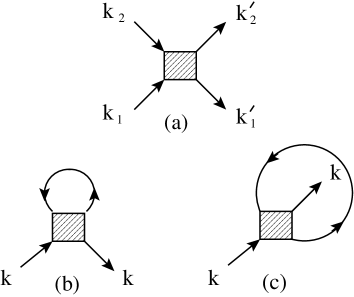
Figure 4: (Color online) (a) Two-body composite fermion interaction with the matrix element $M_{{\bf k}_{1}^{\prime},{\bf k}_{2}^{\prime}}^{{\bf k}_{1},{\bf k}_{2}}$, Eq. (32). (b) Hartree and (c) Fock ways of pairing the operators in the interaction Hamiltonian (31).

In the limit of small density (17) we anticipate the nematic state, discussed qualitatively in section II.3. Choosing its center to be along the positive $x$-direction, one may approximate $\mathrm{arg}({\bf k})\approx k_{y}/k_{0}\ll 2\pi$. We can now employ the form-factors (30) as well as the lower branch dispersion $\varepsilon_{{\bf k},-}$ in the form of Eq. (26), to find for the Hartree-Fock energy

$$K_{\mathrm{HF}}({\bf k})\approx E_{0}+\frac{(k_{x}-k_{0})^{2}}{2m}+\frac{k_{y}^{2}}{2m_{y}}\,,$$ (35)

where

$$m_{y}=m\,\frac{4k_{0}^{2}}{gn}\,\gg m$$ (36)

and $E_{0}=g\sum_{{\bf k}^{\prime}}(k_{y}^{\prime})^{2}n_{{\bf k}^{\prime}}/(4mk_{0}^{2})$ with the effective interaction constant $g=(g_{0}+g_{2})|c|^{2}+2(g_{0}-g_{2})|d|^{2}$. We note here that $m_{y}$ is essentially insensitive to the distribution $n_{k}$, as long as it covers a small fraction of the Rashba circle in the momentum space. It is clear that the Fermi surface, corresponding to the dispersion relation (35) is an ellipse elongated along the $y$ direction and centered around $(k_{0},0)$, Fig. 2. One can now find the chemical potential of interacting fermions at $T=0$ by solving $\sum_{K({\bf k})<\mu_{F}}=n$. This way we find for the chemical potential of the interacting composite fermions

$$\mu_{F}={\frac{5\pi}{4}}\sqrt{g}\,\,\frac{n^{3/2}}{mk_{0}}\,$$ (37)

and $E_{0}=\mu_{F}/5$, in agreement with the estimate in the end of Section III.3.

III.5 Chern-Simons gauge field

So far we have been discussing the interaction energy of the composite fermions. The latter are related to bosons through the Chern-Simons phase according to Eq. (23). We need to discuss now the role of this phase. At the Hartree-Fock level the system is effectively described by non-interacting quasiparticles with the anisotropic dispersion relation Eq. (35). In the coordinate representation the momentum operators are given by $k_{x,y}\to i\partial_{x,y}$. To bring it into a more familiar form one may shift the momentum origin to $(k_{0},0)$ by the gauge factor $e^{ik_{0}x}$ and rescale the variables as $\tilde{x}=\alpha x$ and $\tilde{y}=y/\alpha$, where $\alpha=(m/m_{y})^{1/4}$. In the rescaled coordinates the Hartree-Fock Hamiltonian is isotropic with the cyclotron mass $m_{c}=\sqrt{mm_{y}}$. Upon acting on the Chern-Simons phase the rescaled momentum operator results in a vector potential ${\bf A}(\tilde{\bf r})$, which is included by replacing components of $i\nabla_{\tilde{\bf r}}$ by the corresponding components of $i\nabla_{\tilde{\bf r}}-{\bf A}(\tilde{\bf r})$,

$$H_{\mathrm{HF}}=\sum\limits_{j=1}^{N}{1\over 2m_{c}}\left[(i\partial_{\tilde{x}_{j}}-{\bf A}_{x}(\tilde{\bf r}_{j}))^{2}+(i\partial_{\tilde{y}_{j}}-{\bf A}_{y}(\tilde{\bf r}_{j}))^{2}\right],$$ (38)

where the vector potential is given byNN

$${\bf A}_{\alpha}(\tilde{\bf r}_{j})=\sum\limits_{i\neq j}\epsilon_{\alpha\beta}\,\frac{(\tilde{\bf r}_{j}-\tilde{\bf r}_{i})_{\beta}}{|\tilde{\bf r}_{j}-\tilde{\bf r}_{i}|^{2}}\,,$$ (39)

while the corresponding Chern-Simons magnetic field directed perpendicular to the 2D plane is given by

$$B(\tilde{\bf r}_{j})=\mathrm{curl}{\bf A}(\tilde{\bf r}_{j})={2\pi}\!\sum\limits_{i\neq j}\delta(\tilde{\bf r}_{j}-\tilde{\bf r}_{i})={2\pi}\!\sum\limits_{i\neq j}\delta({\bf r}_{j}-{\bf r}_{i})\,.$$ (40)

To obtain the isotropic form of the Hamiltonian acting in the fermionic space, it is important that the Chern-Simons phase was defined with the rescaled coordinates $\tilde{\bf r}$, Eq. (23). We can now specify the value of the rescaling parameter $\alpha=(m/m_{y})^{1/4}\propto(n/n_{0})^{1/4}\lesssim 1$. Notice that since $m_{y}$ is itself weakly dependent on $\alpha$ (through interaction form-factors $c$ an $d$) the above definition of $\alpha$ is actually a self-consistent equation. Moreover, inclusion of the magnetic field affects the wavefunctions of the quasiparticles, e.g. a homogeneous field results in the Landau quantization. That, in turn, modifies the matrix elements of interactions $M_{{\bf k}_{1}^{\prime},{\bf k}_{2}^{\prime}}^{{\bf k}_{1},{\bf k}_{2}}$ defining $m_{y}$. However, because of the form of interaction $F_{{\bf k}_{1},{\bf k}_{2}}$ and $G_{{\bf k}_{1},{\bf k}_{2}}$ the effective mass appears to depend only weakly on the specific form of the wave functions, as long as those composed of plane waves with wave vectors in the vicinity of the point $(k_{0},0)$. This appears to be the case even for a quantizing magnetic field corresponding to a fully occupied single Landau level. Therefore we use Eq. (36) for $m_{y}$ in the following and apply the effective description Eq. (38) even for a quantizing magnetic field.

The importance of bringing the effective fermionic Hamiltonian to the isotropic form (38) is to argue that the kinetic energy does not contain large logarithms. As explained below Eq. (20), the kinetic energy in presence of the singular magnetic field (40) contain logarithmic integrals. At small distance they are cut by the scale of the correlation hole in the fermionic wavefunction $\Psi_{F}$, while at large distance they are cut by the average distance between the particles. In the isotropic fermionic state described by the Hamiltonian (38) both of these two length scales are given by $k_{F}^{-1}\sim n^{-1/2}$. As a result, the logarithms contain a number rather than a density-dependent parameter. Notice that without rescaling of CS phase such logarithms would contain $\log(1/\alpha)$, making the kinetic energy of the order $n^{3/2}\log(n_{0}/n)$. Rescaling avoids this large extra factor in the kinetic energy.

Keeping the kinetic energy to be $\propto n^{3/2}$ by the fermionic nature of the state along with the careful rescaling of CS phase, suggests to employ the mean-field treatmentJain ; Halperin of CS magnetic field. It substitutes the collection of flux lines (40) by a uniform magnetic field with the same total flux. The latter is given by 2D density of particles (it is important that the rescaling of CS phase is area-preserving and thus not affecting the total flux),

$$B(\tilde{\bf r}_{j})\to B={2\pi}n\,.$$ (41)

The corresponding mean-field vector potential may be chosen as ${\bf A}_{x}(\tilde{\bf r}_{j})=-{\pi}n\tilde{y}_{j}$ and ${\bf A}_{y}(\tilde{\bf r}_{j})={\pi}n\tilde{x}_{j}$. In this approximation the Hamiltonian (38) represents a one-body problem of a particle with the cyclotron mass $m_{c}=\sqrt{mm_{y}}\propto m\sqrt{n_{0}/n}$ in a constant magnetic field (41). The corresponding Landau spectrum is $\varepsilon_{l}=\omega_{c}(l+1/2)$, where $l=0,1,\ldots$ and the cyclotron frequency $\omega_{c}=2\pi n/m_{c}$. Since by construction we introduced exactly one flux quantum per particle, the corresponding filling factor is $\nu=1$. The $N$-body groundstate wavefunction $\Psi_{F}(\tilde{\bf r}_{1},\ldots,\tilde{\bf r}_{N})$ is thus given by the Slater determinant built from the single-particle wavefunctions of the fully occupied lowest Landau level (LLL) (the center of mass shift in the direction of the nematic order produces an additional multiplicative factor $\exp\{ik_{0}\sum_{j}x_{j}\}$). In terms of rescaled complex coordinates $\tilde{z}_{j}=\tilde{x}_{j}+i\tilde{y}_{j}=\alpha x_{j}+iy_{j}/\alpha$ the corresponding fermionic wavefunction takes the formjbook :

$$\Psi_{F}=C_{N}\prod\limits_{i<j}^{N}(\bar{\tilde{z}}_{i}-\bar{\tilde{z}}_{j})\,\,e^{-\pi n\sum\limits_{j}^{N}|\tilde{z}_{j}|^{2}/2}\,e^{ik_{0}\sum\limits_{j}^{N}x_{j}},$$ (42)

where $C_{N}$ is normalization factor. The Chern-Simons phase may be also written in terms of the rescaled complex coordinates as $\prod(\tilde{z}_{i}-\tilde{z}_{j})/|\tilde{z}_{i}-\tilde{z}_{j}|$. As a result the minimal-spin component of the bosonic wavefunction (23) takes the simple form

$$\Psi_{\downarrow\ldots\downarrow}=2^{-N/2}C_{N}\prod\limits_{i<j}^{N}|{\tilde{z}}_{i}-{\tilde{z}}_{j}|\,\,e^{-\pi n\sum\limits_{j}^{N}|\tilde{z}_{j}|^{2}/2}\,e^{ik_{0}\sum\limits_{j}^{N}x_{j}}.$$ (43)

The higher spin components are obtained by acting with the spin raising operators on the minimal spin component, Eq. (III.2). Notice that the spin-raising operator (9) is to be written in non-rescaled original coordinates ${\bf r}_{j}$ to ensure that the wavefunction is projected on the lower SO branch. The wavefunction (43) is independent of the CS chirality $\lambda$. It depends on the single density- and interaction-dependent parameter $\alpha=(m/m_{y})^{1/4}\propto(n/n_{0})^{1/4}$, which specifies the anisotropy. This wavefunction describes an ellipsoidal droplet of the gas elongated along the $x$ direction with the ratio of $x$ and $y$ axes given by $\alpha^{2}$. The average density in this droplet is $n$, while its size depends on the number of particles $N$. The state (43) clearly breaks rotation symmetry. It also breaks time-reversal symmetry as well as parity. Indeed, the parity operation transforms it into the state descendant from the maximal spin component, which is clearly a different, degenerate state. The average energy per particle for the Hamiltonian (38) in such variational $N$-body state is given by

$$\mu_{F}=E_{0}+\varepsilon_{0}={\frac{3\pi}{4}}\sqrt{g}\,\,\frac{n^{3/2}}{mk_{0}}\,.$$ (44)

It indeed confirms the expectation that the composite fermion function of Eqs. (III.2) and (23) yields the energy lower than TRSB and SDW bosonic states.

IV Discussion of the results

IV.1 Phase Diagram

As we have seen, the composite fermion energy per particle is $\mu_{F}\sim\mu_{B}\sqrt{n/n_{0}}$, where $\mu_{B}$, Eq. (15), is the chemical potential of bosonic TRSB and SDW states. Therefore at small density $n\lesssim n_{0}=gk_{0}^{2}$ the composite fermion (CF) groundstate is energetically favorable over bosonic states. On the other hand, at larger density $n\gtrsim n_{0}$ the bosonic states, discussed earlierSAG ; zhai ; Wu ; radic ; ho11 ; Lamacraft ; zhai2 ; yongping ; DasSarma ; ozawa ; ozawa2 ; pitaevskii , have lower energy. We expect thus to observe quantum phase transitions as functions of the chemical potential $\mu$ as well as anisotropy of the interactions $g_{2}$. The corresponding phase diagram is schematically depicted in Fig. 5.

To find out about the nature of the transitions we recall that all three phases break rotational symmetry. In addition TRSB breaks time-reversal, while CF breaks both time-reversal and parity symmetries. We expect thus the first order transition between CF and SDW, where the two discrete symmetries $\hat{T}$ and $\hat{P}$, Eqs. (2), (3), are broken simultaneously. Also the transition between SDW and TRSB, taking place close to $g_{2}=0$, is to be of the first order. Indeed, to avoid density wave modulation in SDW phase the populations of two opposite states on the Rashba circle must be exactly equal. Therefore the transition into TRSB phase with only single populated state must be of the first order.

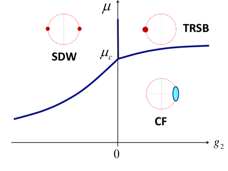
Figure 5: (Color online) Phase diagram of Rashba SO bosons. The full lines are first order transitions. Insets: schematic representation of occupation factors in momentum space (red dots are coherent bosonic condensates, blue ellipse is CF Fermi sea).

Transition from TRSB into CF phase breaks the parity symmetry and could be of the first or second order. One can investigate stability of the bosonic TRSB state against introduction of the small CF component. To this end one can write a variational wavefunction, which contains superposition of TRSB condensate, Eq. (11), with $N_{b}$ particles and nematic CF fraction with $N_{f}\ll N_{b}$ particles and $N_{b}+N_{f}=N$,

$$\Psi({\bf r}_{1},\ldots,{\bf r}_{N}\!)\propto\!\!\sum\limits_{P}\Psi_{B}^{(0)}\!({\bf r}_{1},\ldots,{\bf r}_{N_{b}}\!)\Psi_{CF}\!({\bf r}_{N_{b}+1},\ldots,{\bf r}_{N}\!),$$ (45)

where $P$ stays for a permutation of arguments between $N_{b}$ and $N_{f}$ sets and we have suppressed spin indices for brevity. It is important to realize that the bosonic condensate and a small nematic CF fraction prefer to be on the opposite sides of the Rashba circle, Fig. 5. Indeed this way the spin parts of respective wavefunctions are (almost) orthogonal, minimizing the exchange energy. The residual exchange interactions, due incomplete orthogonality, lead to CF effective mass $m_{y}$ in the direction tangential to the Rashba circle. The energy per unit volume for the state (45) is given by

$$E=\frac{3\pi n_{f}^{2}}{4m_{c}}+\frac{(n-n_{f})^{2}}{2m}\,g_{0}+\frac{(n-n_{f})n_{f}}{m}\,\left[g_{0}+g_{2}\right],$$ (46)

where $n_{f}=N_{f}/N$ and the fermionic cyclotron mass $m_{c}=\sqrt{mm_{y}}=mk_{0}/\sqrt{(g_{0}-g_{2})n/2}$ originates from the exchange interactions of the CF fraction with the bosonic condensate (in the limit $n_{f}\ll n$ the interactions between composite fermions are less important). This mean-field expression shows that for $g_{2}>0$ TRSB state, i.e. $n_{f}=0$, is always the energy minimum and thus it is stable against small CF fraction. An additional energy minimum develops at $n_{f}=n$ for $n<2n_{0}/3\pi$. Although one should not take Eq. (46) as quantitatively accurate beyond $n_{f}\ll n$ limit, it is true that at small enough density the CF phase costs less energy than the bosonic condensates. Together with the local stability of the condensate it suggests the first order transition into the CF phase.

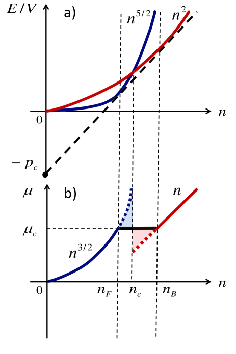
Figure 6: (Color online) (a) Specific energy vs. density for CF and Bose condensate phases. The two graphs intersects at the critical density $n_{c}$. In the range $n_{F}<n<n_{B}$ there is the phase separation. (b) Chemical potential vs. density. Maxwell construction is shown. Compare it to 1D case, Fig. 3.

For the first order transition the equation of state implies the range of density where the Bose condensate (TRSW or SDW) fraction separates from CF fraction. This is illustrated on Fig. 6a. In the region $n_{F}<n<n_{B}$, determined by the common tangential to $E_{F}(n)$ and $E_{B}(n)$, it is energetically favorable to spatially separate the Bose condensate with the fixed density $n_{B}$ from the CF liquid with fixed density $n_{F}$. Changing the total density within this window results in the change between the relative fraction of the two, not changing their individual densities. In terms of the chemical potential vs. density it means a constant critical chemical potential $\mu_{c}$, found from the Maxwell construction, within the window $n_{F}<n<n_{B}$, Fig. 6b. Alternatively, it means a range of a constant critical quantum pressure $p_{c}$, Fig. 6a, on the pressure vs. volume $T=0$ isotherm. To minimize the interfacial energy TRSB and CF fractions prefer to have opposite momenta and spin. This allows avoiding paying the exchange interaction energy thanks to orthogonality of the spinors. One expects thus to find antiferromagnetically ordered mixture of the TRSB Bose condensate and CF fractions.

IV.2 Composite fermion state in a trap

Consider an axially symmetric trap created by a harmonic potential $V(r)=m\omega_{0}^{2}r^{2}$. In the Thomas-Fermi approximation the local density $n(r)$ is found from the condition $V(r)+\mu(n(r))-\mu=0$, where $\mu(n)$ represents microscopic equation of state and $\mu$ is the macroscopic chemical potential, found from the condition $2\pi\int_{0}^{R}rdrn(r)=N$, where $V(R)=\mu$. For CF equation of state $\mu(n)\propto\sqrt{g}n^{3/2}/mk_{0}$, this program yields:

$$\mu\propto\omega_{0}N^{3/5}\left(\frac{g\omega_{0}}{k_{0}^{2}/m}\right)^{1/5},\quad\quad R=\sqrt{\frac{\mu}{m\omega_{0}^{2}}}\propto N^{3/10}.$$ (47)

Here $R$ represents the spatial extent of the $N$-particle groundstate, while $\mu$ is the typical kinetic energy per particle measured upon trap release. These results should be compared with those for the bosonic condensate with the equation of state $\mu(n)\propto gn$. The latter yieldsrmp $\mu\propto\omega_{0}(gN)^{1/2}$ and $R\propto N^{1/4}$. The CF scaling of the chemical potential in the harmonic trap $\mu_{F}\propto N^{3/5}$ is valid as long as it less than the corresponding bosonic result $\mu_{B}\propto N^{1/2}$. Equating the two of them, one finds the condition for the number of particles within the trap below which the CF groundstate prevails

$$N<N_{0}=g^{3}\left(\frac{k_{0}^{2}/m}{\omega_{0}}\right)^{2}.$$ (48)

This is exactly the condition of having the density in the middle of the trap less than the critical one $n(0)<n_{c}$. The density profile acquires the shape $n(r)\propto(R^{2}-r^{2})^{2/3}$. As opposed to the Bose condensate profilepitaevskii $n(r)\propto(R^{2}-r^{2})$, it exhibits infinite slop at the outer edge $r\approx R$.

In experiments of Refs. [Lin-2008, ] and [Lin-2011, ] synthetic gauge field and SO coupling had been engineered with the help of $\lambda=804.1$nm Raman lasers, leading to the typical SO momentum $k_{0}=2\pi/\lambda$ and energy scale $k_{0}^{2}/m\simeq 7$kHz. Taking a trap frequency $\omega_{0}\simeq 30Hz$ as in e.g. Ref. [rolston, ], one obtains $k_{0}^{2}/{m\omega_{0}}\simeq 0.23\times 10^{3}$ and $N_{0}\sim g^{3}\times 10^{5}$. The effective coupling constant $g$ in 2D gas of Rb with $a_{s}=55\AA$ was estimated to beshlyapnikov $g\simeq 0.2$, leading to $N_{0}\simeq 10^{3}$, which is achievable with modern detection techniques. Interestingly enough, studying much smaller particle number experimentally became feasible with the development of single-atom detection technologysingle1 ; single2 .

Since the CF phase has filling factor one, we expect it to be gaped in the bulk of the trap. At the surface it supports a chiral edge mode, which is similar to $\nu=1$ quantum Hall edge. In this sense CF state of Rashba SO bosons is an interacting topological insulator.

At a larger particle number $N>N_{0}$ the middle of the trap has the density exceeding the critical one and thus it reverts to one of the Bose states (TRSB or SDW). The density decays towards the edges of the trap, reaching $n_{B}$ at some radius. Here the phase separation, Fig. 6, takes place and the density discontinuously drops down to $n_{F}$. The outer periphery of the trap contains “vaporized” low-density CF phase, while its inner core is filled with the “liquid” high-density Bose condensate phase. The overall scaling of the chemical potential with the particle number approaches the Bose one, $\mu\sim N^{1/2}$.

IV.3 Rotating systems

The time-reversal and parity broken CF state is chiral. It is not immediately obvious from the minimal spin component wavefunction (43), since it depends on the absolute values $|\tilde{z}_{i}-\tilde{z}_{j}|$ only. However, the spin-raising kernel (9) is certainly chiral and so are all the higher spin components of the many-body bosonic wavefunction (III.2). The degenerate state descending from the maximal spin component (which has exactly the same form as Eq. (43)) has the opposite chirality. The CF groundstate spontaneously breaks the $Z_{2}$ symmetry between them. Rotation of the system serves as an explicit symmetry breaking perturbation, enforcing one of the sates vs. another. Indeed, rotation with the angular frequency $\Omega$ may be viewed as an external magnetic fieldwilkin ${\bf B}_{\mathrm{rot}}=2m_{c}\Omega\hat{\bf z}$, which adds up to CS magnetic field ${\bf B}=\pm 2\pi n\hat{\bf z}$. As a result the total flux is bigger or smaller than one flux quantum per particle, depending on whether CS magnetic filed is parallel or antiparallel with the rotation direction. This either creates $m_{c}\Omega/\pi$ holes per unit area in LLL, or promotes the same number of particles to the next Landau level. At least from the standpoint of the kinetic energy the former alternative requires twice less energy than the latter. One expects thus that the symmetry is broken in a way to add constructively CS and rotational fields to create holes in LLL. Due to presence of these holes, one expects gapless bulk excitations in the rotating system. (Alternatively in analogy with FQHE, excitations may have gaps substantially reduced compared to the $\Omega=0$ case.)

IV.4 Fractional Hall states?

We have employed Chern-Simons phase with one flux quantum per particle to convert composite fermions into bosons, i.e. $\lambda=\pm 1$ in Eq. (23). One could also attach three flux quanta by choosing $\lambda=\pm 3$. This choice leads to the effective magnetic field $B=6\pi n$ and thus to $\nu=1/3$ filling factor. The CF variational groundstate is then given by the Laughlinlaughlin1 state, i.e. $(\bar{\tilde{z}}_{i}-\bar{\tilde{z}}_{j})\to(\bar{\tilde{z}}_{i}-\bar{\tilde{z}}_{j})^{3}$ in Eq. (42). Upon multiplication on CS phase with $\lambda=3$ it leads to the following expression for the minimal spin component

$$\Psi_{\downarrow\ldots\downarrow}\propto\prod\limits_{i<j}^{N}|{\tilde{z}}_{i}-{\tilde{z}}_{j}|^{3}\,\,e^{-3\pi n\sum\limits_{j}^{N}|\tilde{z}_{j}|^{2}/2}\,e^{ik_{0}\sum\limits_{j}^{N}x_{j}},$$ (49)

notice the factor of $3\pi n$ in the exponent which ensures the correct total density $n$. The kinetic energy of such state is factor of three higher than that ascending from Eq. (43). On the other hand, the correlation holes are wider, which may lead to a gain in the interaction energy (especially since the interactions due to higher spin components are essentially non-local). While at the moment we are not aware of a model where the fractional state is advantageous, it is worth pointing out that such a model is in principle possible.

Notice that symmetric minimal spin component may be written with an arbitrary integer exponent $p$ as $\propto\prod_{i<j}^{N}|{\tilde{z}}_{i}-{\tilde{z}}_{j}|^{p}e^{-p\pi n\sum\limits_{j}^{N}|\tilde{z}_{j}|^{2}/2}\,e^{ik_{0}\sum\limits_{j}^{N}x_{j}}$. However only odd $p$’s may be traced to CF construction. This seems to indicate that states with even $p$’s yield larger average energy. This is indeed the case for $p=0$, which is nothing but TRSB condensate with $\mu_{B}\propto n$. It is not clear at the moment how to demonstrate this statement for $p=2,4,\ldots$.

IV.5 Conclusions

We have shown that the low-density phase of Rashba SO bosons may be described as the composite fermion state in the quantizing magnetic filed. Such a state is very different from both TRSB Bose condensate and SDW state discussed before. In particular its equation of state $\mu(n)\propto n^{3/2}$ leads to a different scaling of the kinetic energy and atomic cloud size with the number of particles in shallow traps. It also implies different profile of the cloud density. The excitation spectrum is predicted to be gaped in the bulk of trap with the gapless chiral surface mode at its edge. For deeper traps we predict the phase separation between denser condensate phase in the middle of the trap and dilute CF phase at its edge with the first order density jump at the interface between them.

V Acknowledgments

We are grateful to E. Altman, N. Cooper, G. Juzeliunas, A. Lamacraft and A. Vishwanath for useful discussions. LG thanks Aspen Center for Physics for hospitality. This work was supported by DOE contract DE-FG02-08ER46482.

Appendix A

Here we give details of calculations for the components of the two-particle wavefunction, $\Psi_{\uparrow\uparrow}({\bf r},{\bf r})$ and $\Psi_{\uparrow\downarrow}({\bf r},{\bf r})=\Psi_{\downarrow\uparrow}({\bf r},{\bf r})$ in Eq. (III.3) and derive Eqs. (29), (30) of the main text.

A.1 Calculation of $\Psi_{\uparrow\uparrow}({\bf r},{\bf r})$ and the interaction form-factor $F_{\bf k_{1},k_{2}}$

From Eq. (27) we have

$$\Psi_{\uparrow\uparrow}({\bf r},{\bf r})=$$ (50)

$$\frac{1}{2}\int d{\bf r}_{1}^{\prime}d{\bf r}_{2}^{\prime}{\cal R}({\bf r}-{\bf r}_{1}^{\prime}){\cal R}({\bf r}-{\bf r}_{2}^{\prime})e^{i\lambda\arg({\tilde{\bf r}^{\prime}_{1}}-{\tilde{\bf r}^{\prime}_{2}})}\Psi_{F}({\bf r}_{1}^{\prime},{\bf r}_{2}^{\prime}),$$

where the fermionic part of the wave function is given by

$$\Psi_{F}({\bf r}_{1},{\bf r}_{2})=\frac{1}{\sqrt{2}V}\Big{(}e^{i{\bf k_{1}}{\bf r_{1}}+i{\bf k_{2}}{\bf r_{2}}}-e^{i{\bf k_{2}}{\bf r_{1}}+i{\bf k_{2}}{\bf r_{2}}}\Big{)}$$

and anisotropic vectors ${\tilde{\bf r}^{\prime}_{1}}$ and ${\tilde{\bf r}^{\prime}_{2}}$ in the Chern-Simons factor $e^{i\lambda\arg({\tilde{\bf r}^{\prime}_{1}}-{\tilde{\bf r}^{\prime}_{2}})}$ are defined as ${\tilde{\bf r}^{\prime}_{j}}=(\alpha x_{j}^{\prime},y_{j}^{\prime}/\alpha)$, $j=1,2$, where $\alpha$ is the anisotropy parameter.

To represent the integrand in Eq. (50) in a convenient form, we convert it to the momentum space. Fourier transformation yields

$$e^{i\lambda\arg{\bf\tilde{r}}}=-2\pi i\int\frac{d{\bf k}}{(2\pi)^{2}}\,\frac{e^{i\lambda\arg{\tilde{\bf k}}}}{\tilde{\bf k}^{2}}\,e^{i{\bf k}{\bf r}},$$ (52)

with ${\tilde{\bf k}}=(k_{x}/\alpha,\;\alpha k_{y})$. Fourier image of ${\cal R}({\bf r})$ is ${\cal R}({\bf k})=ie^{-i\arg{\bf k}}$. Substituting now Eqs. (A.1) and (52) into (50), we obtain

$$\Psi_{\uparrow\uparrow}({\bf r},{\bf r})=-\frac{ie^{i({\bf k}_{1}+{\bf k}_{2}){\bf r}}}{4V\sqrt{2}\pi}\int d{\bf k}\,\frac{e^{i\lambda\arg{\tilde{\bf k}}}}{\tilde{\bf k}^{2}}$$ (53)

$$\times\Big{(}e^{-i\arg({\bf k}_{1}+{\bf k})-i\arg({\bf k}_{2}-{\bf k})}-e^{-i\arg({\bf k}_{2}+{\bf k})-i\arg({\bf k}_{1}-{\bf k})}\Big{)}$$

In order to evaluate $F_{{\bf k}_{1}{\bf k}_{2}}$ from (53), it is convenient to introduce the following notations

$$e^{i\lambda\arg{\bf\tilde{k}}} = \frac{k_{x}/\alpha+i\lambda\alpha k_{y}}{|\tilde{k}|}=\left(\frac{\tilde{z}}{|\tilde{z}|}\right)^{\lambda},$$

$$e^{-i\arg({\bf k}_{1}+{\bf k})} = \frac{\bar{w}_{1}+\bar{z}}{|w_{1}+z|},\;\;w_{1}=k_{1,x}+ik_{1,y},$$

$$e^{-i\arg({\bf k}_{2}-{\bf k})} = \frac{\bar{w}_{2}-\bar{z}}{|w_{2}-z|},\;\;w_{2}=k_{2,x}+ik_{2,y},$$

$$z = k_{x}+ik_{y}.$$ (54)

The complex variable $\tilde{z}=k_{x}/\alpha+i\alpha k_{y}$ can be conveniently recast as $\tilde{z}=\frac{z}{2}(\alpha+1/\alpha)+\frac{\bar{z}}{2}(1/\alpha-\alpha)$. Employing integration variables $z$ and $\bar{z}$ and using complex representation of vectors ${\bf k}_{1}$ and ${\bf k}_{2}$, one obtains

$$F_{{\bf k}_{1}{\bf k}_{2}}=\frac{i}{\sqrt{2}}\int\frac{dzd\bar{z}}{4\pi}\frac{1}{|\tilde{z}|^{2}}\Biggl{(}\frac{\tilde{z}}{|\tilde{z}|}\Biggr{)}^{\lambda}\sqrt{\frac{\bar{w}_{1}\bar{w}_{2}}{w_{1}w_{2}}}$$ (55)

$$\times \left[\frac{\frac{\bar{z}^{2}}{\bar{w}_{1}\bar{w}_{2}}-1+\frac{\bar{z}(\bar{w}_{1}-\bar{w}_{2})}{\bar{w}_{1}\bar{w}_{2}}}{\sqrt{|\frac{\bar{z}^{2}}{\bar{w}_{1}\bar{w}_{2}}-1+\frac{\bar{z}(\bar{w}_{1}-\bar{w}_{2})}{\bar{w}_{1}\bar{w}_{2}}}|^{2}}-(w_{1}\longleftrightarrow w_{2})\right].$$

In Eq. (55) the short hand notation $(w_{1}\longleftrightarrow w_{2})$ stands for the same first expression in square brackets but with interchanged variables $w_{1}$ and $w_{2}$.

Upon introducing new dimensionless variables

$$\nu=\frac{z}{\sqrt{w_{1}w_{2}}},\;\;\tau=\frac{w_{1}-w_{2}}{\sqrt{w_{1}w_{2}}},$$ (56)

Eq. (55) yields

$$F_{{\bf k}_{1}{\bf k}_{2}}=-\frac{i}{\sqrt{2}}\sqrt{\frac{\bar{w}_{1}\bar{w}_{2}}{|w_{1}w_{2}|}}\int\frac{d\nu d\bar{\nu}}{4\pi}$$ (57)

$$\times\Biggl{(}\frac{\tilde{\nu}}{|\tilde{\nu}|}\Biggr{)}^{\lambda}\frac{1}{|\tilde{\nu}|^{2}}\Bigg{(}\frac{\bar{\nu}^{2}-1+\bar{\nu}\bar{\tau}}{\sqrt{|\bar{\nu}^{2}-1+\bar{\nu}\bar{\tau}}|^{2}}-(\tau\rightarrow-\tau)\Bigg{)},$$

where $\tilde{\nu}=\frac{\nu}{2}(\alpha+1/\alpha)+\frac{\bar{\nu}}{2}(1/\alpha-\alpha)$ and parameter $\tau$ can be rewritten in terms of original momenta ${\bf k}_{1}$ and ${\bf k}_{2}$ as follows

$$\tau = \sqrt{\frac{k_{1}}{k_{2}}}e^{i(\arg({\bf k}_{1})-\arg({\bf k}_{2}))/2}-\sqrt{\frac{k_{2}}{k_{1}}}e^{-i(\arg({\bf k}_{1})-\arg({\bf k}_{2}))/2}.$$

The integral on the right hand side of (57) is convergent, therefore one can expand the integrand in $\bar{\tau}$ and then perform the integration. Keeping only linear in $\bar{\tau}$ terms in this expansion one finds

$$F_{\bf k_{1},k_{2}}=ic\sqrt{\frac{\bar{w}_{1}\bar{w}_{2}}{|w_{1}w_{2}|}}\,\bar{\tau}\simeq ic\left(e^{-i\arg({\bf k}_{1})}-e^{-i\arg({\bf k}_{2})}\right),$$ (59)

where

$$c_{\lambda}(\alpha)=\int\frac{d\nu d\bar{\nu}}{\sqrt{2}4\pi}\Biggl{(}\frac{\tilde{\nu}}{|\tilde{\nu}|}\Biggr{)}^{\lambda}\frac{1}{|\tilde{\nu}|^{2}}\frac{(|\nu|^{2}-1)({\bar{\nu}}^{2}-1)(\nu+{\bar{\nu}})}{|{\bar{\nu}}^{2}-1|^{3}},$$ (60)

The functions $|c_{\pm}(\alpha)|$ are plotted in Fig. 7.

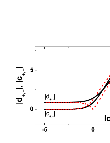
Figure 7: (Color online) Interaction coefficients $|c_{\lambda}(\alpha)|$ and $|d_{\lambda}(\alpha)|$. Full lines correspond to $\lambda=-1$ and dotted lines – to $\lambda=+1$ chirality.

A.2 Calculation of $\Psi_{\uparrow\downarrow}({\bf r},{\bf r})$ and the interaction form-factor $G_{\bf k_{1}k_{2}}$

From Eq. (27) one finds

$$\Psi_{\uparrow\downarrow}({\bf r},{\bf r}) = \frac{1}{2}\int d{{\bf r}_{1}^{\prime}}{\cal R}({\bf r}-{\bf r}_{1}^{\prime})e^{i\lambda\arg({\bf\tilde{r}}^{\prime}_{1}-{\bf\tilde{r}})}\Psi_{F}({\bf r}_{1}^{\prime},{\bf r}),$$

where $\Psi_{F}({\bf r}_{1}^{\prime},{\bf r})$ is defined in Eq. (A.1), while spin-rising operator ${\cal R}$ is given by Eq. (9). After substituting these expressions into (A.2) we obtain

$$\Psi_{\uparrow\downarrow}({\bf r},{\bf r})=\frac{e^{i({\bf k}_{1}+{\bf k}_{2}){\bf r}}}{2V}G_{\bf k_{1}k_{2}},$$

$$G_{\bf k_{1}k_{2}}=-\frac{1}{\sqrt{2}\pi}\!\int\!d{\bf r}^{\prime}\frac{e^{i\lambda\arg({\bf\tilde{r}}-{\bf\tilde{r}^{\prime}})-i\arg({\bf r}-{\bf r^{\prime}})}}{|{\bf r}-{\bf r}^{\prime}|^{2}}$$

$$\times\Big{(}\!e^{-i{\bf k}_{2}({\bf r}-{\bf r}^{\prime})}\!-\!e^{-i{\bf k}_{1}({\bf r}-{\bf r}^{\prime})}\!\Big{)}$$

which shows that $G_{\bf k_{1}k_{2}}$ is a difference of two functions $G_{\bf k_{1}k_{2}}=\tilde{I}_{\bf k_{1}}-\tilde{I}_{\bf k_{2}}$. Introducing $({\bf r-r^{\prime}})_{x}+i({\bf r-r^{\prime}})_{y}=re^{i\phi}$, and $\beta=\log(\alpha)$, we will have for $\lambda=+1$ chirality

$$e^{i\arg({\bf\tilde{r}}-{\bf\tilde{r}^{\prime}})} = \frac{\cosh[\beta]e^{i\phi}+\sinh[\beta]e^{-i\phi}}{|\cosh[\beta]e^{i\phi}+\sinh[\beta]e^{-i\phi}|}$$

$$= \frac{\cosh[\beta]e^{i\phi}+\sinh[\beta]e^{-i\phi}}{\sqrt{\cosh[2\beta](1+\tanh[2\beta]\cos[2\phi])}}.$$

Importantly, the form-factor corresponding to the $\lambda=-1$ chirality can be obtained by interchanging $\cosh[\beta]$ with $\sinh[\beta]$ in the numerator of Eq. (A.2). Then we obtain

$$\tilde{I}_{\bf k}=\frac{1}{\pi\sqrt{2\cosh[2\beta]}}$$

$$\times \int\frac{dr}{r}d\phi\frac{(\cosh[\beta]+\sinh[\beta]e^{-2i\phi})e^{-ikr\cos[\phi-\arg({\bf k})]}}{\sqrt{1+\tanh[2\beta]\cos[2\phi]}}.$$

We note that the integral $\tilde{I}_{\bf k}$ has a logarithmical divergent contribution coming from $r\rightarrow 0$, but it cancels out in the difference $\tilde{I}_{\bf k_{1}}-\tilde{I}_{\bf k_{2}}$ and therefore in $G_{\bf k_{1}k_{2}}$. In order to find the coefficient $d_{\lambda}(\alpha)$ in Eq. (30) we need to evaluate integral (A.2) in linear over $\arg({\bf k})\ll 2\pi$ approximation. Upon expanding integrand over $\arg({\bf k})$ and integrating over $r$ we arrive to the following expression

$$d_{\lambda}(\alpha)=\frac{is_{\lambda}}{\pi\sqrt{2\cosh[2\beta]}}\int_{0}^{2\pi}d\phi\frac{1-\cos[2\phi]}{\sqrt{1+\tanh[2\beta]\cos[2\phi]}},$$

where $s_{+}=\sinh[\beta]$ and $s_{-}=\cosh[\beta]$. The function $|d_{\pm}(\alpha)|$ is plotted vs $\ln\alpha$ for both chiralities $\lambda=\pm 1$ in Fig. 7.

References

- (1) Y.-J. Lin, R. L. Compton, A. R. Perry, W. D. Phillips, J. V. Porto, and I. B. Spielman, Phys. Rev. Lett. 102, 130401 (2009).
- (2) Y.-J. Lin, R. L. Compton, K. Jimenez-Garcia, J. V. Porto, and I. B. Spielman, Nature 462, 628 (2009).
- (3) Y-J. Lin, R. L. Compton, K. Jimenez-Garcia, W. D. Phillips, J. V. Porto, and I. B. Spielman, Nature Phys. 7, 531 (2011).
- (4) Y.-J. Lin, K. Jimenez-Garcia, and I. B. Spielman, Nature 471, 83 (2011).
- (5) Jin-Yi Zhang, Si-Cong Ji, Zhu Chen, Long Zhang, Zhi-Dong Du, Bo Yan, Ge-Sheng Pan, Bo Zhao, Youjin Deng, Hui Zhai, Shuai Chen, Jian-Wei Pan, arXiv:1201.6018v2.
- (6) Y. A. Bychkov and E. I. Rashba, J. Phys. C 17 , 6039 (1984).
- (7) G. Dresselhaus, Phys. Rev., 100, 580 (1955).
- (8) J. Stenger, S. Inouye, D. M. Stamper-Kurn, H.-J. Miesner, A. P. Chikkatur, and W. Ketterle, Nature 396, 345 (1998).
- (9) T.-L. Ho, Phys. Rev. Lett. 81, 742 (1998).
- (10) C. K. Law, H. Pu, and N. P. Bigelow, Phys. Rev. Lett. 81, 5257 (1998).
- (11) A. B. Kuklov and B. V. Svistunov, Phys. Rev. Lett. 89, 170403 (2002).
- (12) S. Ashhab and A. J. Leggett, Phys. Rev. A 68, 063612 (2003).
- (13) D. Jaksch and P. Zoller, New.J. Phys. 5, 56 (2003).
- (14) T. D. Stanescu, C. Zhang, and V. Galitski, Phys. Rev. Lett. 99, 110403 (2007).
- (15) T. D. Stanescu, B. Anderson, and V. Galitski, Phys. Rev. A 78, 023616 (2008).
- (16) J. Ruseckas, G. Juzeliunas, P. Ohberg and M. Fleischhauer, Phys. Rev. Lett. 95, 010404 (2005).
- (17) K. Osterloh, M. Baig, L. Santos, P. Zoller, and M. Lewenstein, Phys. Rev. Lett. 95, 010403 (2005).
- (18) S. L. Zhu, H. Fu, C. J. Wu, S. C. Zhang, and L. M. Duan, Phys. Rev. Lett. 97, 240401 (2006).
- (19) G. Juzeliunas, J. Ruseckas, and J. Dalibard, Phys. Rev. A 81, 053403 (2010).
- (20) D. L. Campbell, G. Juzeliunas, and I. B. Spielman, Phys. Rev A 84, 025602 (2011).
- (21) J. Dalibard, F. Gerbier, G. Juzeliunas, and P. Ohberg, Rev. Mod. Phys. 83, 1523 (2011).
- (22) B. M. Anderson, G. Juzeliunas, V. M. Galitski, and I. B. Spielman, Phys. Rev. Lett. 108, 235301 (2012).
- (23) C. Wang, C. Gao, C.-M. Jian, and H. Zhai, Phys. Rev. Lett. 105, 160403 (2010).
- (24) C. Wu, I. Mondragon-Shem, X. F. Zhou, Chin. Phys. Lett. 28, 097102 (2011).
- (25) J. Radic’, T. A. Sedrakyan, I. B. Spielman, and V. Galitski, Phys. Rev. A 84, 063604 (2011).
- (26) T.-L. Ho and S. Zhang, Phys. Rev. Lett. 107, 150403 (2011).
- (27) S. Gopalakrishnan, A. Lamacraft, and P. M. Goldbart, Phys. Rev. A 84, 061604(R) (2011).
- (28) H. Zhai, Int. J. Mod. Phys. B 26 1230001 (2012).
- (29) Y. Zhang, L. Mao, and C. Zhang, Phys. Rev. Lett. 108, 035302 (2012).
- (30) T.Ozawa, and G. Baym, Phys. Rev. Lett. 109, 025301 (2012).
- (31) T.Ozawa, and G. Baym, arXiv:1207.5263v1.
- (32) R. Barnett, S. Powell, T. Gra, M. Lewenstein, and S. Das Sarma, Phys. Rev. A 85, 023615 (2012).
- (33) Y. Li, L. P. Pitaevskii, and S. Stringari, Phys. Rev. Lett. 108, 225301 (2012).
- (34) Y. K. Kato, R. C. Myers, A. C. Gossard, and D. D. Awschalom, Science 306, 1910 (2004).
- (35) M. Z. Hasan and C. L. Kane, Rev. Mod. Phys. 82, 3045 (2010).
- (36) N. Nagaosa, J. Sinova, S. Onoda, A. H. MacDonald, and N. P. Ong, Rev. Mod. Phys. 82, 1539 (2010).
- (37) I. Zutic, J. Fabian, and S. Das Sarma, Rev. Mod. Phys. 76, 323(2004).
- (38) L. Tonks, Phys. Rev. 50, 955 (1936).
- (39) M. Girardeau, J. Math. Phys. 1, 516 (1960).
- (40) E. H. Lieb and W. Liniger, Phys. Rev. 130, 1605 (1963).
- (41) M. Flicker and E. H. Lieb, Phys. Rev. 161, 179 (1967).
- (42) C. N. Yang, Phys. Rev. Lett. 19, 1312 (1967).
- (43) M. Gaudin, Phys. Lett. A 24, 55 (1967).
- (44) E. Berg, M. S. Rudner and S. Kivelson, Phys. Rev. B 85, 035116 (2012).
- (45) J. K. Jain, Phys. Rev. Lett. 63, 199 (1989).
- (46) A. Lopez and E. Fradkin, Phys. Rev. B 44, 5246 (1991).
- (47) B. Halperin, P. A. Lee and N. Read, Phys. Rev. B 47, 7312 (1993).
- (48) S. Das Sarma and A. Pinczuk, Perspectives in Quantum Hall Effects: Novel Quantum Liquids in Low Dimensional Semiconductor Structures. New York: Wiley-VCH, (1996). ISBN 978-0-471-11216-7.
- (49) O. Heinonen, Composite Fermions. Singapore: World Scientific, (1998). ISBN 981-02-3592-5.
- (50) J.K. Jain, Composite Fermions. New York: Cambridge University Press, (2007). ISBN 978-0-521-86232-5.
- (51) S. D. Huber and E. Altman, Phys. Rev. B 82, 184502 (2010).
- (52) P. Nozieres, Theory Of Interacting Fermi Systems, West view press, (1997).
- (53) F. Dalfovo, S. Giorgini, L. P. Pitaevskii, and S. Stringari, Rev. Mod. Phys. 71, 463 (1999).
- (54) N. R. Cooper, N. K. Wilkin, and J. M. F. Gunn, Phys. Rev. Lett. 87, 120405 (2001).
- (55) M.C. Beeler, M.E.W. Reed, T. Hong, and S.L. Rolston, New J. Phys. 14, 073024 (2012).
- (56) D. S. Petrov, M. Holzmann, and G.V. Shlyapnikov, Phys. Rev. Lett. 84, 2551 (2000).
- (57) C. Weitenberg, M. Endres, J. F. Sherson, M. Cheneau, P. Schaub, T. Fukuhara, I. Bloch, and S. Kuhr, Nature 471, 319 (2011).
- (58) P. Wurtz, T. Langen, T. Gericke, A. Koglbauer, and H. Ott, Phys. Rev. Lett. 103, 080404 (2009).
- (59) R. B. Laughlin, Phys. Rev. Lett. 50, 1395 (1983).