A Light Stop with Flavor in Natural SUSY

Roberto Auzzi, Amit Giveon, Sven Bjarke Gudnason and Tomer Shacham

Racah Institute of Physics, The Hebrew University, Jerusalem, 91904, Israel

Abstract

The discovery of a SM-like Higgs boson near 125 GeV and the flavor texture of the Standard Model motivate the investigation of supersymmetric quiver-like BSM extensions. We study the properties of such a minimal class of models which deals naturally with the SM parameters. Considering experimental bounds as well as constraints from flavor physics and Electro-Weak Precision Data, we find the following. In a self-contained minimal model – including the full dynamics of the Higgs sector – top squarks below a TeV are in tension with $b\to s\gamma$ constraints. Relaxing the assumption concerning the mass generation of the heavy Higgses, we find that a stop not far from half a TeV is allowed. The models have some unique properties, e.g. an enhancement of the $h\to b\bar{b},\tau\bar{\tau}$ decays relative to the $h\to\gamma\gamma$ one, a gluino about 3 times heavier than the stop, an inverted hierarchy of about $3\div 20$ between the squarks of the first two generations and the stop, relatively light Higgsino neutralino or stau NLSP, as well as heavy Higgses and a $W^{\prime}$ which may be within reach of the LHC.

 
auzzi(at)phys.huji.ac.il
giveon(at)phys.huji.ac.il
gudnason(at)phys.huji.ac.il
tomer.shacham(at)phys.huji.ac.il

1 Introduction

The discovery of a SM-like Higgs boson at the LHC [1, 2] provides us with the last of the eighteen SM parameters. We take this as an opportunity to (re)consider models Beyond the Standard Model (BSM) addressing naturally the full texture of the SM. A perturbative Higgs near 125 GeV points towards a supersymmetric (SUSY) extension of the SM as a possible explanation to the hierarchy problem. The Minimal Supersymmetric extension of the SM (MSSM), however, requires the stop to be heavier than 5 TeV without sizable $A$-terms (see e.g. [3, 4]), in order to radiatively generate the appropriate quartic term in the Higgs potential. On the other hand, such a heavy stop does not cut off the quadratic divergences of top loops at a sufficiently low energy and, consequently, a tuning at the per-mille level is necessary [5, 6]. This tension hints for a supersymmetric extension with a mechanism to crank up the mass of the lightest CP-even Higgs, $m_{h_{0}}$.

Furthermore, the direct search for missing transverse energy (MET) is pushing up the bounds on the masses of the first generation squarks to be well above the TeV [7]. The second generation squarks typically need to be very close to that of the first generation in order to pass the bounds coming from meson mixings. The bounds on the third generation squarks, however, remain much weaker [8]. This experimental fact together with the desire to alleviate fine tuning calls for an inverted hierarchy of sparticle masses. This is sometimes called effective SUSY, natural SUSY or more minimal SUSY [9, 10, 11, 12, 13, 14, 15]. For concrete models realizing this scenario, see e.g. [16, 17, 18, 19, 20, 21, 22, 23, 24, 25, 26, 27, 28, 29, 30].

In this paper we consider a quiver-like extension of the Supersymmetric Standard Model (SSM), which essentially consists of two copies of the SM gauge group (${\rm U}(1)\times{\rm SU}(2)\times{\rm SU}(3)$) with appropriate link fields connecting them, see fig. 1. The link fields acquire a VEV via the Higgs mechanism, breaking the gauge symmetry down to that of the SM. If the Higgsing of the link fields takes place near a few TeV, non-decoupling of the D-terms will contribute to the Higgs quartic coupling at tree level. This contribution alone may allow for a 126 GeV Higgs [31, 32, 20, 33, 34, 23, 27].

Interestingly, such extensions of the SM may also address the flavor problem [20, 23, 27] by choosing the messengers of SUSY breaking and the chiral superfields of the first two generations, $q_{1,2}$, to be connected to node $B$, while the matter of the third generation, $q_{3}$, and the Higgs superfields, $H_{u,d}$, are charged under node $A$, see fig. 1. This automatically gives rise to a flavor texture in the fermion sector, with a hierarchy between the third and the first two generations, due to the structure of irrelevant gauge-invariant terms, which are suppressed by the UV scale of flavor dynamics [20, 23]. The precise flavor texture depends on the representations $R$ of the link fields $\omega,\tilde{\omega}$ in fig. 1. This was analyzed in detail in [23], where it was shown that in several cases, the SM parameters are naturally obtained, and the flavor constraints are satisfied. Furthermore, this construction gives rise also to the above-mentioned inverted hierarchy between the first/second and third generation sfermions. As the first and second generations are charged under the same gauge group as the messenger fields, they acquire masses as in gauge mediation, while the third generation masses are suppressed as in gaugino mediation [35, 36, 37, 38, 39, 40, 41, 42, 43].

We are interested in natural models and choose to define this statement by allowing fine tuning of UV parameters in the Lagrangian [5, 6] of only down to the percent level, but no further. Conventionally, this concept is tightly connected to the Higgs sector. Here we consider a broader version of the argument where we do not allow the tuning of any parameter in all sectors of the Lagrangian to be tuned more than at the percent level (using a similar definition as in the Higgs sector); this includes the parameters describing the flavor and CP violating operators etc. Concretely, we consider a sparticle spectrum to be natural if the following criteria are met: the stops are lighter than about a TeV; the gluino weighs less than about $3$ times the stop mass [14]; $\mu<200$ GeV.

The scope of this paper is to investigate – within the class of models described above and with the mentioned naturalness criteria – the question of how light the stop mass can be for spectra passing all present collider bounds, electroweak precision tests and flavor constraints. A relatively light stop (in the ballpark of half a TeV), can only exist if the other squarks are much heavier. Remarkably, such an inverted hierarchy is automatic in the model of fig. 1. If the VEV of the link field $v=\langle\omega\rangle$ is smaller or of the order of the messenger scale $M$, then the squarks of the 3rd generation are indeed much lighter than the other squarks. A self-contained minimal model – including the dynamics of the Higgs sector – has the following properties. A light stop is tied with a small $m_{H_{d}}^{2}$; the latter is in tension with $b\to s\gamma$ constraints. We consequently find that the stop below a TeV in the self-contained minimal model is in tension with experiment. On the other hand, treating $m_{H_{d}}^{2}$ as a free parameter at the messenger scale, we find that the stop can be accommodated in the $600\div 1000$ GeV range. Having the Higgs at 126 GeV as well as light stops yields typically a “light” $W^{\prime}$ vector boson, near $4\div 10$ TeV. Furthermore, the model typically has either a Higgsino neutralino NLSP or sometimes a stau NLSP near 100 GeV. Interestingly, this class of models has relatively heavy electroweak gaugini making it possible for the self-contained version of the model to explain [20] the $\mu/B\mu$ problem providing a reasonable $\tan\beta$ without any further dynamics in the Higgs sector.

The paper is organized as follows. In sec. 2, we present an overview of the general properties of the minimal construction of fig. 1, while in sec. 3, we present the details of the model as well as the results of the paper. In sec. 4, we contemplate an extension that may unify in the standard way (as opposed to accelerated unification [44] or the type studied in [27], which may be applied also to the minimal model of sec. 2). We conclude with a discussion, and some details are presented in the appendices.

2 Overview of the minimal model

Figure 1: A diagram describing the minimal model with gauge groups $G_{A},G_{B}={\rm U}(1)\times{\rm SU}(2)\times{\rm SU}(3)$ and link fields $\omega,\tilde{\omega}$. SUSY breaking is connected via messenger fields $T,\tilde{T}$ only to $G_{B}$.

The model of BSM physics we study is characterized by the following scales. SUSY breaking is communicated to the visible sector of the model at the messenger scale $M$. The visible sector consists of two copies of the SM gauge group which are connected by certain link fields $\omega,\tilde{\omega}$, see fig. 1. The link fields are chosen in representations such that when they acquire a VEV $\langle\omega\rangle=\langle\tilde{\omega}\rangle=v$, they Higgs the two gauge groups down to the low-energy SM group. Above the messenger scale $M$, we contemplate an appropriate UV completion involving certain dynamics responsible for creating the flavor texture of the SM, which we however only parametrize by higher-dimension operators all suppressed by the scale $\Lambda_{\rm flavor}\gtrsim M$. The models of the type we consider can have a UV completion in terms of a deformed SQCD where $\Lambda_{\rm flavor}$ then is the strong coupling scale of the latter theory [40]. We will consider the case where $\Lambda_{\rm flavor}\gtrsim M\gg v$ with $v$ near the weak scale; it is however constrained by electroweak precision tests (EWPTs) to be typically above 1.5 TeV.

The matter content of the theory is arranged as follows. The first and second generation matter fields are charged under the group $G_{B}$ (see fig. 1) while the Higgses and the third generation are charged under the group $G_{A}$. The superpartner masses for the matter on the node $G_{B}$ are given (for $v\ll M$) as in minimal gauge mediation [45], while those of $G_{A}$ are suppressed by $v/M$ as in gaugino mediation [35, 36, 37, 38, 39, 40, 41, 42, 43]:

$$m_{\tilde{Q}_{1,2},\tilde{u}_{1,2},\tilde{d}_{1,2},\tilde{L}_{1,2},\tilde{e}_{1,2}}\simeq M_{1,2,3}\simeq{\rm a\ few\times}\mu_{\rm EW}\,,\qquad m_{\tilde{Q}_{3},\tilde{u}_{3},\tilde{d}_{3},\tilde{L}_{3},\tilde{e}_{3}}\simeq B\mu\simeq 0\,,$$ (1)

at the messenger scale $M$. $M_{1,2,3}$ are the (heavy) gaugino masses. The low-energy masses of the third generation and those of the Higgses are all generated via RG evolution which in turn requires a sufficiently heavy gluino etc. The $\mu$ term however is generated by a higher dimension operator [20],

$$\mathcal{W}_{\mu}\sim\frac{\omega\tilde{\omega}}{\Lambda_{\rm flavor}}H_{u}H_{d}\,,$$ (2)

which for $\Lambda_{\rm flavor}\approx 100$ TeV gives $\mu$ of the right order of magnitude, viz. of the weak scale $\mu_{\rm EW}$.

Only the third generation SM fermions receive a mass at tree level, explaining the large top, bottom and tau mass with respect to the other ones. The hierarchy between the top and the bottom is provided by $\tan\beta$. The remaining part of the SM fermions acquires masses via higher-dimension operators involving the link fields $\omega,\tilde{\omega}$. The representation of the link fields determines the Yukawa texture of the SM fermions. In the simplest case the link fields are bifundamental fields of ${\rm SU}(5)$, transforming as $({\bf 5},\bar{\bf 5})$ under the two gauge groups $G_{A}\times G_{B}$ (which decomposes as a field $({\bf 2},\bar{\bf 2})_{\frac{1}{2},-\frac{1}{2}}$ under ${\rm SU}(2)\times{\rm U}(1)$ which we denote $\omega_{L}$ and as $({\bf 3},\bar{\bf 3})_{\frac{1}{3},-\frac{1}{3}}$ under ${\rm SU}(3)\times{\rm U}(1)$ which we call $\omega_{d}$). The higher dimensional representation $({\bf 10},\overline{\bf 10})$ gives rise to a somewhat better flavor texture [23] while also adding a lot of matter fields which can pose problems in terms of a Landau pole. In this paper we will stick to the simplest link fields, namely those transforming as $({\bf 5},\bar{\bf 5})$. An example of such a higher-dimension operator is

$$\frac{\lambda_{ij}^{u}}{\Lambda_{\rm flavor}}Q_{i}H_{u}u_{j}^{c}\omega_{L}\,,\qquad i,j=1,2,\ (\rm generation\ indices)\,,$$ (3)

producing Yukawa textures schematically as [20, 23]

$$Y_{u}\sim\begin{pmatrix}\epsilon&\epsilon&\epsilon^{2}\\ \epsilon&\epsilon&\epsilon^{2}\\ \epsilon^{2}&\epsilon^{2}&1\end{pmatrix}\,,\qquad Y_{d}\sim\begin{pmatrix}\epsilon&\epsilon&\epsilon^{2}\\ \epsilon&\epsilon&\epsilon^{2}\\ \epsilon&\epsilon&1\end{pmatrix}\,,\qquad Y_{e}\sim\begin{pmatrix}\epsilon&\epsilon&\epsilon\\ \epsilon&\epsilon&\epsilon\\ \epsilon^{2}&\epsilon^{2}&1\end{pmatrix}\,,\qquad\epsilon\equiv\frac{v}{\Lambda_{\rm flavor}}\,,$$ (4)

for the up, down and LH lepton sectors, respectively. The matrices should be understood as the order of magnitude of the higher-dimension operators, viz. each element is multiplied by its own order-one coefficient. An appropriate set of order-one numbers can reproduce the measured quark masses as well as the CKM matrix [23].

Concerning phases we impose CP conservation at the messenger scale $M$ such that all the gaugino masses are real valued. RG evolution does not change this. Further phases in the Higgs sector could a priori be of concern, however, we tackle those together with a solution to the $\mu/B\mu$ problem. $\mu$ is generated by the higher-dimension operator (2) giving roughly the 100 GeV scale (and it runs very slowly during RG), while $B\mu$ is negligible at the scale $M$ but is generated via RG evolution ($B\mu$ is a SUSY-breaking parameter and receives contributions comparable to the other fields on node $G_{A}$, hence it is very suppressed at the scale $M$). $B\mu$ turns out to be rather small in other models with this type of mechanism, however since in our model the gaugini are necessarily rather heavy, a sufficiently large $B\mu$ (of order $\mu^{2}$) is obtained, giving rise to acceptable values of $\tan\beta$. This way of generating $B\mu$ ensures that the CPV phase arg$(\mu^{*}B\mu)$ is negligible.

As mentioned, the gluino is quite heavy in our model, due to the fact that while the stop is very light at the messenger scale, a sizable stop mass is needed for driving the up Higgs tachyonic in time for EWSB to happen. This means that the gluino has to be sufficiently heavy as to feed enough mass into the stop so EWSB occurs, but not too heavy so fine-tuning is sufficiently small. Another characteristic coming along with the negligible masses on the node $G_{A}$ at the scale $M$ is that the down Higgs is typically small in the model if no additional contribution is contemplated which in turn renders the heavy Higgses rather light, of the order of less than 400 GeV.

Finally, let us mention that even though the gluino weighs in pretty well and we typically find the stops in the range of $400\div 1000$ GeV, the Higgsino mass $\mu$ is generically as low as 100 GeV – all in all giving rise to just a little fine tuning in the model at hand.

Clearly, we wish to obtain the complete low-energy spectra and in turn what predictions can be drawn from those. Since we have heavy link fields $\omega,\tilde{\omega}$ as well as two gauge groups between the scales $M$ and $v$ we implement a custom made RG code that evolves the running masses at two loops and gauge couplings at one loop down to $v$. The light third generation receives an extra contribution due to a threshold effect of integrating out the heavy gaugini and link fields [46]. After Higgsing we sum up everything and plug in the evaluated masses to the spectrum calculator SOFTSUSY which we use to calculate the pole masses of the particles. Since starting with arbitrary model parameters at the messenger scale $M$, it is not likely to provide a spectrum which is not ruled out by experimental constraints or is not far from them. In order to put the model on the edge of exclusion (or discovery, depending on the point of view), we apply direct search constraints as well as electroweak precision tests (EWPTs) to the evaluated spectrum to determine whether it matches what we just described. The direct search bounds we apply are from both LEP, Tevatron and the LHC and are applied to the chargini, neutralini, gluino, first and second generation squarks, stau, stau neutrino and CP-odd Higgs $A_{0}$. The indirect limits are applied to the charged Higgses $H_{\pm}$ (from flavor measurements of $b\to s\gamma$), and the oblique $T$ parameter limits on the VEV $v$ (up to a combination of the gauge couplings) as well as the soft mass of the link fields. We also consider a larger set of EWPTs setting (somewhat independent) limits also on $v$. Now when a spectrum is calculated, we calculate an error value based on asymmetric potentials (with large coefficients) pushing the spectrum towards the allowed region with respect to the limits. The bottom of this potential consists basically of the stop mass. Finally, we use educated guesses for the starting point as well as a steepest descent algorithm to find a spectrum with as low stop masses as possible in a spectrum satisfying all desired constraints. This will be presented in sec. 3.7.

Let us sum up what we found. As mentioned the heavy Higgses ($H_{\pm}$) turn out to be generically too light with respect to the flavor constraint coming from $b\to s\gamma$ (at more than $95\%$ CL.). Ignoring this fact, we can accommodate the stops near 600 GeV with the gluino weighing in at around 3 times that value, i.e. near 2 TeV. Taking into account the $b\to s\gamma$ constraint at 2 sigma, pushes up the stops to around 1000 GeV and correspondingly the gluino to roughly 3 TeV. Of course we should take this constraint seriously, however, the reason for cutting it some slack is the general concern that $\mu/B\mu$ in some cases might require some extra dynamics above or at the messenger scale $M$, which could provide further contributions to the Higgs masses. Indeed by pushing up the down Higgs $H_{d}$ it is possible to crank up the heavy Higgses and hence the $H_{\pm}$ mass beyond the flavor limit. Having this option in mind, we leave open the possibility that the stops can be as light as 550 GeV. The heavy squarks, viz. those of the first and second generations are commonly $5\div 17$ times heavier than the stops and hence rather safe for flavor constraints such as those coming from $K-\bar{K}$, $B-\bar{B}$, and $D-\bar{D}$ mixings. Insisting that the model be free of further dynamics in the Higgs sector, we can avoid the $b\to s\gamma$ limits by pushing up the scales. In this case, interestingly, the $B\mu$ term can be generated at the right order of magnitude as to have a reasonable $\tan\beta\sim 10\div 25$. Since the $\mu$ term is generated by the higher-dimension operator (2), this provides a solution to the $\mu/B\mu$ problem at the price of the stops being near or slightly above the TeV.

The predictions of the models are the following. In this natural SUSic setting we can have the stop near $600\div 1100$ GeV. The $\mu$ parameter is generically 100 GeV or so and there are typically very light neutralini, chargini, staus and stau neutrino, in the ballpark of $100\div 250$ GeV. Even though it might be some challenge for the LHC this would be a thrill for the ILC. The NLSP in the model can be either the lightest stau or the (mostly Higgsino) neutralino. Furthermore, this model giving rise to the flavor texture of the SM as well as an inverted hierarchy of sparticles comes with $B^{\prime}$, $W^{\prime}$ and $g^{\prime}$ vector particles. The $W^{\prime}$s are typically the lightest with a mass of roughly

$$m_{W^{\prime}}\gtrsim 2v\,,$$ (5)

where $v$ is typically near 2 TeV, and the saturation being at equal ${\rm SU}(2)$ couplings of the two nodes $G_{A},G_{B}$.

This concludes our overview of the model. The reader interested in the details of the model is invited to read on, while the others may jump to sec. 3.7. In sec. 4, we describe an extension of the model which allows standard unification (as opposed to accelerated unification which may be applied to the minimal model as well).

3 Details of the minimal model

The model shown in fig. 1 has qualitatively all the ingredients for providing a successful phenomenology including a relatively heavy Higgs particle – at 126 GeV – as well as a light stop. We have in mind a low scale mediation scenario with the Higgsing of the link fields taking place near the electroweak scale. The model provides heavy first and second generation squarks as they are situated close to SUSY breaking, while the third generation squarks are light as they have suppressed masses due to the link fields as in gaugino mediation. The third generation fermions are heavy as they are placed on the same node as the Higgs fields while the first and second generation fermions acquire masses via higher dimension operators and hence are much smaller. Finally, in the low scale mediation case, non-decoupled D-terms increase the tree-level Higgs mass, alleviating the need for heavy stops or large $A$-terms.

3.1 Parameter space

As mentioned in the introduction we seek to search for the lightest possible stops in the parameter space of the above described model. In order to cover as large a part of the parameter space as possible, we invoke doublet-triplet splitting both in the messenger sector and in the link sector. The parameter space is thus parametrized in terms of the variables described below. We consider a minimal messenger sector

$$\mathcal{W}_{T}=\sum_{i=1}^{n_{\rm mess}}\left[S_{2}T_{i2}\tilde{T}_{i2}+S_{3}T_{i3}\tilde{T}_{i3}\right]\,,\qquad\langle S_{2}\rangle=\eta M+\theta^{2}F\,,\qquad\langle S_{3}\rangle=M+\theta^{2}F\,,$$ (6)

where the messengers $T_{i2},\tilde{T}_{i2}$ transform as ${\bf 2}_{-\frac{1}{2}},\bar{\bf 2}_{\frac{1}{2}}$ under ${\rm SU}(2)_{L}\times{\rm U}(1)_{Y}$, respectively, while $T_{i3},\tilde{T}_{i3}$ transform as ${\bf 3}_{-\frac{1}{3}},\bar{\bf 3}_{\frac{1}{3}}$ under ${\rm SU}(3)_{c}\times{\rm U}(1)_{Y}$, respectively. The link field sector with doublet-triplet splitting provides the following mass-squared matrix for the gauge bosons

$$\mathcal{M}^{2}_{v_{k}}=2v_{k}^{2}\begin{pmatrix}g_{A_{k}}^{2}&-g_{A_{k}}g_{B_{k}}\\ -g_{A_{k}}g_{B_{k}}&g_{B_{k}}^{2}\end{pmatrix}\,,$$ (7)

with eigenvalues $0$ and

$$m_{v_{k}}^{2}=2\left(g_{A_{k}}^{2}+g_{B_{k}}^{2}\right)v_{k}^{2}\,,$$ (8)

where $k=1,2,3$ stand for ${\rm U}(1)$, ${\rm SU}(2)$ and ${\rm SU}(3)$, respectively. The link fields are bifundamental fields $\{\omega_{d},\omega_{L}\}$ as are their conjugates $\{\tilde{\omega}_{d},\tilde{\omega}_{L}\}$. Here we are using the notation of [23] for the link fields where $\omega_{R},\tilde{\omega}_{R}$ denote a pair of fields transforming under the representation $R,\bar{R}$ of $G_{A}$ and as $\bar{R},R$ of $G_{B}$, respectively; $R$ is written in terms of a SM field in such a representation. The VEVs of the link fields are

$$\langle\omega_{d}\rangle=\langle\tilde{\omega}_{d}\rangle=v_{3}\,,\qquad\langle\omega_{L}\rangle=\langle\tilde{\omega}_{L}\rangle=v_{2}\,,\qquad v_{1}^{2}=\frac{3}{5}v_{2}^{2}+\frac{2}{5}v_{3}^{2}\,,$$ (9)

from which we define the parameters

$$y_{k}=\frac{m_{v_{k}}}{\sqrt{\eta}M}\,,\qquad y\equiv\left(y_{1}y_{2}y_{3}\right)^{\frac{1}{3}}\,,\qquad\kappa=\frac{v_{2}}{v_{3}}\,.$$ (10)

At the Higgsing scale $m_{v_{k}}$ the standard model gauge couplings $g_{k}$ are given by

$$\frac{1}{g_{k}^{2}}=\frac{1}{g_{A_{k}}^{2}}+\frac{1}{g_{B_{k}}^{2}}\,,$$ (11)

from which it is practical to define the following three angles

$$\tan\theta_{k}\equiv\frac{g_{A_{k}}}{g_{B_{k}}}\,.$$ (12)

Finally, we define

$$x=x_{3}\equiv\frac{F}{M^{2}}\,,\qquad x_{2}\equiv\frac{F}{\eta M^{2}}\,.$$ (13)

In summary, the parameter space is parametrized by the set of variables $\{M,x,y,\eta,\kappa,\theta_{k},n_{\rm mess}\}$.

3.2 SUSY-breaking masses

The gaugino masses are similar to those of minimal gauge mediation [47], however with doublet-triplet splitting taken into account,

$$m_{\tilde{g}_{k}}=n_{\rm mess}\left(\frac{g_{k}}{4\pi}\right)^{2}\Lambda_{k}\,q(x)\,,\qquad q(x)=\frac{1}{x^{2}}\left[(1+x)\log(1+x)+(1-x)\log(1-x)\right]\,,$$ (14)

where $n_{\rm mess}$ is the number of copies of messengers and the effective SUSY breaking scales are given by

$$\Lambda_{3}=\frac{F}{M}\,,\qquad\Lambda_{2}=\frac{F}{\eta M}\,,\qquad\Lambda_{1}=\frac{3}{5}\Lambda_{2}+\frac{2}{5}\Lambda_{3}\,.$$ (15)

The sfermion masses are given in eq. (4.2) of [48],

$$m_{\tilde{f}_{l}}^{2} =2n_{\rm mess}\bigg{[}\left(\frac{g_{3}}{4\pi}\right)^{4}\Lambda_{3}^{2}\,C_{2,3}^{\tilde{f}}\,\mathcal{E}^{l}(x_{3},y_{3},\lambda_{3})+\left(\frac{g_{2}}{4\pi}\right)^{4}\Lambda_{2}^{2}\,C_{2,2}^{\tilde{f}}\,\mathcal{E}^{l}(x_{2},y_{2},\lambda_{2})$$

$$\phantom{=2n_{\rm mess}\bigg{[}}+\left(\frac{g_{1}}{4\pi}\right)^{4}\bigg{(}\frac{2}{5}\Lambda_{3}^{2}\,C_{2,1}^{\tilde{f}}\,\mathcal{E}^{l}(x_{3},y_{1},\lambda_{1})+\frac{3}{5}\Lambda_{2}^{2}\,C_{2,1}^{\tilde{f}}\,\mathcal{E}^{l}(x_{2},y_{1}\lambda_{1})\bigg{)}\bigg{]}\ ,$$ (16)

where $C_{2,k}^{\tilde{f}}$, $k=1,2,3$, is the quadratic Casimir of the representation under which the sfermion ${\tilde{f}}$ transforms, while the index $l$ runs over generations. The function $\mathcal{E}^{l}$ for the first and second generations is given by [48]

$$\mathcal{E}^{1,2}(x,y,\lambda_{k}) =\frac{1}{x^{2}}\bigg{[}\alpha_{0}(x)-\left(1-\lambda_{k}^{2}\right)\alpha_{1}(x,y)-(1-\lambda_{k})^{2}y^{2}\alpha_{2}(x,y)-\frac{2(1-\lambda_{k})}{y^{2}}\beta_{-1}(x)+\beta_{0}(x)$$

$$\phantom{=\frac{1}{x^{2}}\bigg{[}\ }+\frac{2(1-\lambda_{k})}{y^{2}}\beta_{1}(x,y)+(1-\lambda_{k})^{2}\beta_{2}(x,y)\bigg{]}\,,\qquad\lambda_{k}\equiv\frac{1}{\sin^{2}\theta_{k}}\,,$$ (17)

whereas for the third generation it reads

$$\mathcal{E}^{3}(x,y)=\frac{1}{x^{2}}\left[\alpha_{0}(x)-\alpha_{1}(x,y)-y^{2}\alpha_{2}(x,y)-\frac{2}{y^{2}}\beta_{-1}(x)+\beta_{0}(x)+\frac{2}{y^{2}}\beta_{1}(x,y)+\beta_{2}(x,y)\right]\,.$$ (18)

The $\alpha$s and $\beta$s are defined in app. A of [48]. The soft mass of the link fields is also given by eq. (16), with $\mathcal{E}^{\rm link}=\mathcal{E}^{1}+\mathcal{E}^{3}$ and an appropriate quadratic Casimir (see [48] for details). Note that we work in part of the parameter space where $y\sim 1/100$ or so and hence the above formulae can to a good approximation be described as $\mathcal{E}^{1,2}$ being that of minimal gauge mediation [47] and $\mathcal{E}^{3}\sim 0$. In our studies we use the full formulae even though the spectra obtained are not really sensitive to the mentioned approximation.

3.3 RG evolution

In order to calculate particle spectra we need to evaluate the RG running from the messenger scale – which we take to be the geometric average of that of the two messenger fields: $\sqrt{\eta}M$ – down to the Higgsing scale of the link fields $m_{v}\equiv y\sqrt{\eta}M$. The beta function coefficients of the gauge couplings read

$$b_{A_{1}}=5\,,\quad b_{A_{2}}=-1\,,\quad b_{A_{3}}=-4\,,\quad b_{B_{1}}=\frac{33}{5}\,,\quad b_{B_{2}}=0\,,\quad b_{B_{3}}=-2\,,$$ (19)

while the beta functions for the masses in the model are given in app. A. In the above we have assumed that the doublet-triplet splittings in the messenger sector and the link sector are small enough that running from the average messenger scale to the average Higgsing scale is a sufficiently good approximation.

3.4 Threshold effects

At scale $m_{v}$ the sfermion masses of the node $G_{A}$ (viz. the third generation ones) receive a contribution from integrating out the link fields and the heavy gaugini [46],

$$\delta m_{\tilde{f}}^{2}=\sum_{k}\left(\frac{g_{k}}{4\pi}\right)^{2}C_{\tilde{f},k}\left[2\sin^{2}\theta_{k}(1-3\sin^{2}\theta_{k})M_{k,B}^{2}+m_{v_{k}}^{2}\tan^{2}\theta_{k}\log\left(1+\frac{2m_{\omega_{k}}^{2}}{m_{v_{k}}^{2}}\right)\right]\,,$$ (20)

where $m_{\omega_{3}}$ is the soft mass of $\omega_{d},\tilde{\omega}_{d}$ and $m_{\omega_{2}}$ is that of $\omega_{L},\tilde{\omega}_{L}$ while $m_{\omega_{1}}^{2}=\frac{3}{5}m_{\omega_{2}}^{2}+\frac{2}{5}m_{\omega_{3}}^{2}$. The soft masses of the Higgs fields at the scale $m_{v}$ receive the following contribution,

$$\delta m_{H_{u,d}}^{2}=\delta m_{\tilde{L}}^{2}+\left(\frac{\lambda_{t,b}g_{3}}{4\pi^{2}}\right)^{2}\left[2\sin^{4}\theta_{3}M_{\tilde{g},B}^{2}-\frac{1}{2}m_{v_{3}}^{2}\tan^{2}\theta_{3}\log\left(1+\frac{2m_{\omega_{3}}^{2}}{m_{v_{3}}^{2}}\right)\right]\,,$$ (21)

where $\lambda_{t,b}$ are the Yukawa couplings of the top and bottom, respectively.

3.5 Higgs sector

In order to naturally acquire a Higgs mass of 126 GeV, we exploit the fact that in the part of parameter space of interest, the D-terms do not decouple completely in the presence of SUSY breaking,

$$V_{D}=\frac{g_{2}^{2}(1+\Delta_{2})}{8}\left|H_{u}^{\dagger}\sigma^{a}H_{u}+H_{d}^{\dagger}\sigma^{a}H_{d}\right|^{2}+\frac{3}{5}\frac{g_{1}^{2}(1+\Delta_{1})}{8}\left|H_{u}^{\dagger}H_{u}-H_{d}^{\dagger}H_{d}\right|^{2}\,,$$ (22)

where $\sigma^{a}$ are the Pauli matrices and

$$\Delta_{k}=\tan^{2}\theta_{k}\frac{2m_{\omega_{k}}^{2}}{m_{v_{k}}^{2}+2m_{\omega_{k}}^{2}}\,,$$ (23)

yielding tree-level Higgs masses [31, 27]

$$m^{2}_{h_{0},H_{0}} =\frac{1}{2}\left(m^{2}_{A_{0}}+\tilde{m}^{2}\mp\sqrt{(m^{2}_{A_{0}}-\tilde{m}^{2})^{2}+4\tilde{m}^{2}m^{2}_{A_{0}}\sin^{2}(2\beta)}\right)\,,$$ (24)

$$m_{H^{\pm}}^{2} =m_{A_{0}}^{2}+m_{W}^{2}(1+\Delta_{2})\,,\qquad m_{A_{0}}^{2}=2|\mu|^{2}+m_{H_{u}}^{2}+m_{H_{d}}^{2}\,,$$ (25)

where the $\mu$ term is corrected as

$$|\mu|^{2}=-\frac{1}{2}\tilde{m}^{2}-\frac{m_{H_{u}}^{2}\tan^{2}\beta-m_{H_{d}}^{2}}{\tan^{2}\beta-1}\,.$$ (26)

The mass parameter $\tilde{m}$ is given by

$$\tilde{m}^{2}=\frac{\frac{3}{5}g_{1}^{2}(1+\Delta_{1})+g_{2}^{2}(1+\Delta_{2})}{2}\,v_{h}^{2}\,,\qquad v_{h}=174\,{\rm GeV}\,,$$ (27)

in terms of which the tree-level bound on the Higgs mass reads [31, 32, 20]

$$m_{h_{0}}^{2}<\tilde{m}^{2}\,.$$ (28)

We furthermore assume that $B\mu$ is zero at the messenger scale $M$ and is generated by RG running

$$B\mu\simeq-\mu\left(\frac{3g_{2}^{2}}{8\pi^{2}}M_{2}\log\frac{m_{v_{2}}}{M_{2}}+\frac{3g_{1}^{2}}{40\pi^{2}}M_{1}\log\frac{m_{v_{1}}}{M_{1}}\right)\,,$$ (29)

where $M_{1,2}$ are gaugino masses. By generating $B\mu$ dynamically it is no longer possible to choose $\tan\beta$, which hence is determined by

$$\sin 2\beta=\frac{2B\mu}{m_{A_{0}}^{2}}\,.$$ (30)

We denote by

$$r_{x}=\frac{g_{hxx}}{g_{hxx}^{SM}}\,,\qquad x=t,b,\tau,V,G,\gamma\,,$$ (31)

the effective Higgs couplings normalized to the respective SM one and

$$\mu_{x}=\frac{\sigma\times{\rm BR}(x)}{\sigma\times{\rm BR}(x)_{\rm SM}}\,,\qquad x=t,b,\tau,V,G,\gamma\,,$$ (32)

is the signal strength in each experimental channel. The tree-level couplings (see e.g. [49]) are rescaled as

$$r_{b}=r_{\tau}=-\frac{\sin\alpha}{\cos\beta}\,,\qquad r_{t}=\frac{\cos\alpha}{\sin\beta}\,,\qquad r_{V}=\sin(\beta-\alpha)\,,$$ (33)

where the parameter $\alpha$ is defined as the mixing angle between $(H_{0d},H_{0u})$ as in the MSSM [50] and is given by

$$\tan 2\alpha=\frac{m^{2}_{A_{0}}+\tilde{m}^{2}}{m^{2}_{A_{0}}-\tilde{m}^{2}}\tan 2\beta\,.$$ (34)

The corrections to $g_{h\gamma\gamma}$ and $g_{hGG}$ come from one-loop diagrams; in the region of parameters studied in this paper, the deviations from the standard model are quite negligible (see [51, 52] for a recent discussion).

The only Higgs couplings which can have a sizable modification are

$$r_{b}=r_{\tau}\approx 1+2\frac{\tilde{m}^{2}}{m^{2}_{A_{0}}}\,,$$ (35)

where the approximation is valid for large $\tan\beta$ and to the leading order in $\tilde{m}/m_{A_{0}}$. When $m_{H\pm}$ saturates the bound of 380 GeV from $b\to s\gamma$, this gives $r_{b},r_{\tau}\approx 1.2$. This could enhance the signal strengths, $\mu_{b}\simeq\mu_{\tau}\simeq 1.12$, which in turn would suppress $\mu_{\gamma}\simeq 0.78$. This is in some tension with current experimental data, in which $h\to\gamma\gamma$ is enhanced [1, 2, 53, 54, 55, 56, 57, 58, 59].

3.6 Constraints

There are various constraints that we have to take into account in finding viable spectra, which we now describe in turn. The constraints come in two types; direct search bounds and indirect limits such as the oblique parameters, other electroweak precision tests (EWPTs) and flavor constraints.

In the class of direct constraints, we consider the bounds on the first and second generation squarks as function of the gluino mass [7]. For instance for a 1.5 TeV gluino, the first and second generation squarks should be heavier than 1.5 TeV and heavier than 1.75 TeV for a 1 TeV gluino (see fig. 7 in [7]). Our spectra do in general obey these constraints, so this particular constraint is not really limiting our search. For the stau and the mostly Higgsino neutralino, the only bounds we can apply are due to LEP, hence $m_{\tilde{\tau}_{1}}>82$ GeV and $m_{\tilde{\chi}_{1}^{0}}>46$ GeV. The latter is never needed for the spectra at hand.

Searches for $\gamma\gamma+$MET put a bound on the chargino $m_{\tilde{\chi}_{1}^{\pm}}>270$ GeV [60, 61] in the case of a mostly bino NLSP (the lightest neutralino being mostly bino and the lightest chargino thus mostly wino). This situation typically happens when $\mu$ is not sufficiently light, whereas when $\mu<200$ GeV, both the lightest chargino and the lightest neutralino are Higgsini and hence the NLSP is typically a Higgsino neutralino. In this case the bound on the chargino that applies is the LEP bound reading $m_{\tilde{\chi}_{1}^{\pm}}>94$ GeV [62].

Among the oblique parameters, $T$ is the important one and it receives contributions from a diagram of Higgses exchanging a ${\rm U}(1)$ boson and a triplet scalar coming from the bifundamental ${\rm SU}(2)$ link field after it is Higgsed (${\bf 2}\otimes{\bf 2}={\bf 1}\oplus{\bf 3}$). This amounts to

$$\Delta T=\frac{v_{h}^{2}}{\alpha}\left[\frac{3}{20}\frac{\sin^{4}\theta_{1}}{v_{1}^{2}}+\frac{g_{A_{2}}^{4}v_{2}^{2}\cos^{2}(2\beta)}{\left(2(g_{A_{2}}^{2}+g_{B_{2}}^{2})v_{2}^{2}+2m_{\omega_{2}}^{2}\right)^{2}}\right]\,,\qquad v_{h}=174\;{\rm GeV}\,,$$ (36)

which by neglecting the first term and assuming $|\cos(2\beta)|\simeq 1$, we can rewrite as

$$\left(1+\cot^{2}\theta_{2}\right)\frac{v_{2}}{v_{h}}+\frac{m_{\omega_{2}}^{2}}{g_{A_{2}}^{2}v_{2}v_{h}}>\frac{1}{\sqrt{4\alpha|\Delta T|}}\simeq\frac{5.9}{0.07+0.08n}\,,$$ (37)

where the equality assumes a face value of $T=0.07$ [62] and $n$ is the number of standard deviations one wishes to allow. We choose to work with model points within roughly $1.5\sigma$.

Other electroweak tests are relevant as well; while not expressed in terms of oblique parameters, they are typically parametrized using a (higher-dimension) operator basis, where the limits are applied to the respective coefficients via a chi-squared fit to electroweak precision data. The Lagrangian density of the higher-dimension operators takes the form $\delta\mathcal{L}=a_{X}\mathcal{O}_{X}$, with $X$ being the operator in question. The operators relevant here are [63, 64] $\mathcal{O}_{h}=|h_{0}^{\dagger}D_{\mu}h_{0}|^{2}$, $\mathcal{O}^{t}_{\psi\psi^{\prime}}=(\bar{\psi}\gamma^{\mu}\sigma^{a}\psi)(\bar{\psi}^{\prime}\gamma_{\mu}\sigma^{a}\psi^{\prime})$, $\mathcal{O}^{t}_{h\psi}=i(h_{0}^{\dagger}\sigma^{a}D^{\mu}h_{0})(\bar{\psi}\gamma_{\mu}\sigma^{a}\psi)+{\rm h.c.}$, $\mathcal{O}^{s}_{\psi\psi^{\prime}}=(\bar{\psi}\gamma^{\mu}\psi)(\bar{\psi}^{\prime}\gamma_{\mu}\psi^{\prime})$, $\mathcal{O}^{s}_{h\psi}=i(h_{0}^{\dagger}D^{\mu}h_{0})(\bar{\psi}\gamma_{\mu}\psi)+{\rm h.c.}$, with coefficients

$$a_{h} =-\frac{\alpha}{v_{h}^{2}}\Delta T\,, \qquad a^{t}_{\psi\psi^{\prime}} =-\frac{1}{8v_{2}^{2}}\cos^{4}\theta_{2}\,,$$ (38)

$$a^{t}_{\psi\Psi^{\prime}} =a^{t}_{h\psi}=\frac{1}{8v_{2}^{2}}\sin^{2}\theta_{2}\cos^{2}\theta_{2}\,, \qquad a^{t}_{h\Psi} =-\frac{1}{8v_{2}^{2}}\sin^{4}\theta_{2}\,,$$ (39)

$$a^{s}_{\psi\psi^{\prime}} =-\frac{3}{10v_{1}^{2}}Y_{\psi}Y_{\psi^{\prime}}\cos^{4}\theta_{1}\,, \qquad a^{s}_{\psi\Psi^{\prime}} =\frac{3}{10v_{1}^{2}}Y_{\psi}Y_{\Psi^{\prime}}\sin^{2}\theta_{1}\cos^{2}\theta_{1}\,,$$ (40)

$$a^{s}_{h\psi} =\frac{3}{20v_{1}^{2}}Y_{\psi}\sin^{2}\theta_{1}\cos^{2}\theta_{1}\,, \qquad a^{s}_{h\Psi} =-\frac{3}{20v_{1}^{2}}Y_{\Psi}\sin^{4}\theta_{1}\,,$$ (41)

where $\psi$ is a 1st or 2nd generation SM fermion, while $\Psi$ is a third generation one. We use a chi-squared fit with data of [64] to limit the operator coefficients to within the $3\sigma$ level.

A CMS search for neutral Higgs bosons decaying to tau pairs has been able to exclude $A_{0}$ up to 450 GeV for $\tan\beta=45$, and 290 GeV for $\tan\beta=20$, while for $\tan\beta$ below $7\div 8$ no additional limit (to that of LEP) has been obtained, see fig. 3 in [65]. For $\tan\beta=7$ we required $m_{A_{0}}>125$ GeV while for $\tan\beta=20$, $m_{A_{0}}>290$ GeV.

Constraints from $b\to s\gamma$, by comparing experiment to NNLO QCD (at second order in the strong coupling), set the bound $m_{H_{\pm}}>380$ GeV at $95\%$ CL [66]. This new constraint is a lot more restrictive than the former one [67]. The choice of conforming with the brand new limit pushes up the spectra to some degree. We checked, using the expressions in [68], that the contributions to the $b\to s\gamma$ branching ratio mediated by superpartners are negligible in the region of parameters relevant for the benchmark points (the bound on $m_{H\pm}$ changes only at the percent level).

The heavy gauge bosons may also mediate FCNC; the most dangerous constraints come from $g^{\prime}$, due to a stronger gauge coupling. These contributions are suppressed by the small non-diagonal elements of the matrices which diagonalize the Yukawa couplings in eq. (4); constraints from meson mixings are usually satisfied for $v_{3}\gtrsim 2$ TeV with $\theta_{3}\approx\pi/4$.

3.7 Benchmark points

Finally, we are ready to sum up the contributions to all the soft masses described in secs. 3.2–3.5, which we plug into SOFTSUSY 3.3.0 [69] in order to make the final RG evolution from the scale $m_{v}$ down to the electroweak scale, providing us with benchmark points describing the characteristics of the model. Fig. 2a shows a benchmark point with a 126 GeV Higgs and as light stop $\tilde{t}_{1}$ as we have been able to find in parameter space.

 

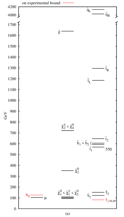
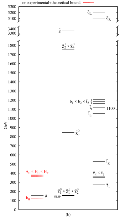
Figure 2: (a) An example with a light stop; the heavy Higgs masses can be placed arbitrarily (in the range of $\sim 350\div 1000$ GeV) by choosing $m_{H_{d}}^{2}$ at the messenger scale $M$ – this freedom has a negligible effect on the rest of the spectrum. (b) An example of superpartners and Higgs masses in a self-contained minimal model – including the Higgs sector all of whose soft masses, including $B\mu$, are dynamically generated – that has a natural SM flavor texture; more details are given in appendix B.

Let us dwell a bit on the NLSP of the model under study. Typically it is the (RH) stau or the Higgsino neutralino, depending on the point in parameter space. Often the points with a stau NLSP come hand in hand with a small VEV $v_{2}$ and correspondingly a relatively light $W^{\prime}$ which typically is at odds with the EWPTs. It is theoretically also possible that the stau neutrino is the NLSP, which can happen also in a very small (and experimentally excluded) corner of minimal gauge mediation. We find however that all such points are excluded by EWPTs (maybe a particular corner is still allowed by limits).

The mechanism giving rise to a light stau neutrino is the following. In this model $L_{3}$ typically has a larger mass than $e_{3}$ and this typically does not change even after the two-loop running from the messenger scale down to the Higgsing scale. However, taking into account the threshold effects of eq. (20) it is possible that the field $e_{3}$ receives a significantly larger boost than $L_{3}$ when integrating out the link fields because $m_{\omega_{1}}$ can be far larger than $m_{\omega_{2}}$. This is due to the hypercharge squared of $e_{3}$ being four times bigger than that of $L_{3}$ and hence if the threshold effect coming from integrating out the link field $\omega_{2}$ is small enough, the RH stau can become heavier than the LH stau and thus the stau neutrino can in principle be the NLSP.

The heavier Higgses, $H_{0},A_{0},H_{\pm}$, are typically light in our model as it stands. Having light “heavy Higgses” (of the order of $\sim 350$ GeV) is a prediction in the minimal incarnation of the model if we do not allow additional dynamics in the Higgs sector to contribute to the soft masses of the Higgses. This is constrained by $b\to s\gamma$ and has consequences for the signal strength of Higgs decays. In this minimal version of the model the stop typically needs to be around the TeV in order for the spectrum to satisfy the constraints on the Higgs sector (see fig. 2b). If on the other hand we allow for additional contributions to the soft masses of the Higgses at or above the messenger scale, then it is possible to leave the stop as light as $\sim 550$ GeV (see fig. 2a). For instance, increasing only the soft mass $m_{H_{d}}^{2}$ can push up the “heavy Higgses” above experimental bounds leaving the rest of the spectrum more or less unchanged.

Electroweak symmetry breaking (EWSB) is not per se an issue in the model as it stands. However, the fact that all the soft masses of the third generation as well as those of the Higgses start out negligible at the messenger scale and acquire everything by RG evolution constrains the gluino to weigh in at a certain level. This minimum mass of the gluino, by means of the model, sets a lower bound on the stops. We find that the lightest stop is typically heavier than $500$ GeV, consistent with the analysis of [27]. Notice that the gluino mass is also typically heavy in the model as it is related to the soft masses of the first and second generation squarks and link fields which need to be heavy to make $\Delta_{1,2}$ large and avoid the collider bounds. The most limiting constraint on the stop mass, however, comes from the fact that it is correlated with the NLSP (often a RH stau) which has to satisfy the LEP bound.

In order to allow for a natural texture in the fermion sector of the model, we consider fixing the following parameters [20],

$$\epsilon_{2}=\frac{v_{2}}{\Lambda_{\rm flavor}}=0.02\,,\qquad\epsilon_{3}=\frac{v_{3}}{\Lambda_{\rm flavor}}=0.07\,,$$ (42)

where $\Lambda_{\rm flavor}$ is the UV scale where flavor texture is generated. An inspection of the CKM matrix reveals that the $\epsilon$s have to be large enough to reproduce the Cabibbo angle. If this is not the case, the order one numbers of the higher-dimension operators illustrated in eq. (4) have to be rather large. As $y_{k}=m_{v_{k}}/M\simeq 3v_{k}/M$ and it is required that $\Lambda_{\rm flavor}\gtrsim M$, eq. (42) puts a lower bound on $y_{k}\gtrsim 3\epsilon_{k}$, with $k=2,3$. A spectrum with appropriately chosen $y$s such as to allow for the above $\epsilon$s is shown in fig. 2b.

The example in fig. 2b provides the spectrum of our self-contained minimal model – including the Higgs sector where all its soft masses, including $B\mu$, are dynamically generated – which has a natural flavor texture and satisfies all direct as well as indirect experimental bounds. The tuning of the Higgs mass-squared is at the percent level in this case.

4 Extension with unification

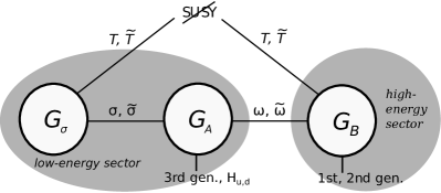
Figure 3: A diagram describing the model with gauge groups $G_{\sigma}={\rm SU}(2)$, $G_{A}={\rm U}(1)\times{\rm SU}(2)\times{\rm SU}(3)$, $G_{B}={\rm SU}(5)$ and link fields $\sigma,\tilde{\sigma},\omega,\tilde{\omega}$. The ${\rm SU}(2)$ node is added to enhance the Higgs mass.

We now present an extension of the minimal model described in sec. 3, which allows for gauge coupling unification [31]. The model is described by the quiver-like diagram in fig. 3. The outline of the extended model is as follows. The messenger scale is set near the GUT scale, $M\sim M_{\rm GUT}$, and SUSY breaking is communicated via messengers from a single secluded sector to both group $G_{B}=SU(5)$ and $G_{\sigma}=SU(2)$ (hence the model has a single spurion). The VEV of the link fields $\omega,\tilde{\omega}$ is also taken to be near the GUT scale, such that $y_{\omega}$ is order 1; this is sufficient to generate the required inverted hierarchy in the sparticle spectrum. However, the soft masses of the $\omega$-type link fields are negligible relative to their Higgsing scale, and consequently their contribution to $\Delta_{1,2}$ is negligible. Hence the VEV of the bifundamental link fields $\sigma,\tilde{\sigma}$ needs to be relatively near the electroweak scale, namely $y_{\sigma}\sim 10^{-11}$ or smaller. This can in principle give rise to tachyonic (LH) staus due to the large range of running of the link fields $\sigma,\tilde{\sigma}$. The link fields need to be sufficiently heavy in order for the $\Delta$s to be of order one, such that the lightest CP-even Higgs mass can be placed near 125 GeV. A counteracting mechanism is also at work, since by cranking up $y_{\omega}$, the soft masses on the $G_{A}=G_{\rm SM}$ node are increased. This in turn pushes up the stop mass and can then become a problem for naturalness in the model. All this said, the model in principle provides a viable unifying theory with a light stop and a 126 GeV Higgs.

Let us comment on the possibilities for unification and flavor texture. The link fields $\omega,\tilde{\omega}$ could be chosen to transform in the ${\bf 5},\bar{\bf 5}$ of ${\rm SU}(5)$ or alternatively in the ${\bf 10},\overline{\bf 10}$ which is much better for flavor physics [23]. These representations will not prohibit the gauge coupling unification of the group $G_{A}$ as they are complete representations of ${\rm SU}(5)$ and also these links will run only a little bit. The group $G_{B}$ is already chosen as an ${\rm SU}(5)$ and nothing needs to be done here. One can further speculate on the unification of the “low-energy sector” of fig. 3. The exceptional group ${\rm E}_{6}$ contains ${\rm SU}(2)\times{\rm SU}(6)$ which in turn contains ${\rm SU}(2)\times{\rm U}(1)\times{\rm SU}(2)\times{\rm SU}(3)$. This is all what is needed for the low-energy sector. It is also possible to consider the so-called trinification group ${\rm SU}(3)^{3}$ which is a subgroup of ${\rm E}_{6}$. This however requires the low-energy sector to be embedded in ${\rm E}_{8}$ as it contains ${\rm SU}(3)\times{\rm E}_{6}$.

Finally, we make an estimate to see whether the many decades of running can make the (LH) staus tachyonic. Using the two-loop beta functions of app. A and the threshold corrections (20), taking into account the wino, the heavy 1st and 2nd generation squarks as well as the link fields $\sigma,\tilde{\sigma}$, we obtain the running mass for the (LH) stau at the scale $m_{v_{\sigma}}$ (assuming it starts out vanishing)

$$\delta m_{L_{3}}^{2} =\frac{3\alpha_{2}}{8\pi\cos^{2}\theta_{\sigma}}\bigg{[}\Upsilon\log y_{\sigma}+\sin^{2}\theta_{\sigma}\bigg{]}m_{\sigma}^{2}\,,$$ (43)

$$\Upsilon \equiv\frac{\alpha_{2}}{\pi\cos^{2}\theta_{\sigma}}\left(\frac{1}{3}\left(\frac{4\alpha_{3}}{\alpha_{2}}\right)^{2}\frac{\sin^{4}\theta_{\sigma}}{\sin^{4}\theta_{\omega,3}}+4\frac{\tan^{4}\theta_{\sigma}}{\sin^{4}\theta_{\omega,2}}+2\right)-\frac{8n_{\rm mess}}{3}\sin^{4}\theta_{\sigma}\,,$$

where $g_{\sigma}=g_{2}/\sin\theta_{\sigma}$, $m_{\sigma}^{2}$ is the soft mass of the link fields $\sigma,\tilde{\sigma}$ and $\alpha_{k}=g_{k}^{2}/(4\pi)$. We have neglected all contributions proportional to $\alpha_{1}$ and we have assumed that the effective SUSY-breaking scale $F/M$ is the same on both node $G_{\sigma}$ and $G_{B}$.

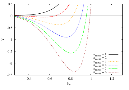
Figure 4: $\Upsilon$ as function of $\theta_{\sigma}$ for various numbers of messengers $n_{\rm mess}$; here $\theta_{\omega,2}=\theta_{\omega,3}=\pi/4$.

Fig. 4 shows the value of $\Upsilon$ in eq. (43) as function of $\theta_{\sigma}$ and number of messengers $n_{\rm mess}$ for $\theta_{\omega,2}=\theta_{\omega,3}=\pi/4$. Whenever $\Upsilon$ is negative, any $y_{\sigma}<1$ (even parametrically small) is free of problems with tachyons. The range for $\theta_{\sigma}$ is chosen such that $\alpha_{\sigma},\alpha_{A+B,2}<1/2$ both remain perturbative. For $n_{\rm mess}=1$, $\Upsilon$ is positive definite while for $n_{\rm mess}>1$ it is negative for some range of $\theta_{\sigma}$. For $\theta_{\sigma}=\pi/4$, $\Upsilon$ is negative for $n_{\rm mess}\geq 3$.

5 Discussion

In this paper we answered the question of how light the stop can be in minimal supersymmetric quiver-like extensions of the SM, which deal with all the eighteen SM parameters, including a 126 GeV Higgs boson, and which satisfy all current experimental bounds. The answer depends on whether we allow for additional dynamics modifying the soft masses of the Higgs sector or we assume that the model be self contained. If we allow modification of the Higgs masses we can accommodate the stop near 550 GeV, while in a self-contained model as it stands, the stop cannot be lighter than roughly a TeV. In this latter version, the $B\mu$ term is radiatively generated due to heavy electroweak gaugini allowing for a reasonably low $\tan\beta\sim 20$. The heavy gaugini come along with a heavy gluino, and the latter gives rise to some residual tuning.

We find that the properties of the spectra are rather robust. A relatively light stop, near the $0.5\div 1$ TeV range, is accompanied by a heavy gluino, with mass $m_{\tilde{g}}\sim 3m_{\tilde{t}}$, heavy 1st and 2nd generation squarks, a factor of $3\div 20$ heavier than the stop, and a relatively light $W^{\prime}$, in the $3\div 10$ TeV range. The NLSP is either a light Higgsino neutralino or a stau, near 100 GeV; in the latter case, the $W^{\prime}$ is lighter, and may be within the reach of the LHC. It may also be possible to obtain a stau neutrino NLSP in some corners of parameter space, though we did not manage to find an example that satisfies all our constraints.

We have performed the search for the lightest possible third generation squarks without applying direct search limits to them a priori. After we obtained the results we then checked whether the stops or sbottoms (which are typically degenerate in our model) are excluded or close to being discovered. In the regime of parameters studied in this paper, the NLSP decays to a gravitino inside the detector; the direct search limit (with only $2.05\;{\rm fb}^{-1}$ of integrated luminosity at $\sqrt{s}=7$) for a 100 GeV neutralino and other colored sparticles decoupled requires $m_{\tilde{t}_{1}}\gtrsim 270$ GeV [70]. All our results comply with this limit, but the spectra with the lightest stops (and additional contribution to the heavy Higgses) could be discovered (or excluded) in the near future by the LHC.

The model as it stands is the minimal version and it does not allow for a standard unification, though in some region of parameter space it may allow for some type of accelerated unification [44, 27]. We have therefore contemplated some extension with more gauge groups and link fields which may unify in the standard way, to perhaps an ${\rm E}_{n}\times{\rm E}_{m}$ GUT. We leave a detailed study thereof for the future.

Finally, let us discuss the predictions obtained via coupling to the Higgs sector. In the case where the heavy Higgses are as light as allowed by direct and indirect experimental constraints, i.e. near 380 GeV, the effective Higgs couplings to $\tau\bar{\tau}$ and $b\bar{b}$ are enhanced by roughly $20\%$. Hence the signal strength in $h\to b\bar{b},\tau\bar{\tau}$ increases by roughly $12\%$ which in turn decreases that of $h\to\gamma\gamma$ by $22\%$. An enhancement of the $h\to b\bar{b},\tau\bar{\tau}$ decay relative to the $h\to\gamma\gamma$ one is thus a prediction of the model. This may be in tension with the enhanced $h\to\gamma\gamma$ branching ratio suggested by current experimental data [1, 2]. However, the measurements are limited by significant theoretical uncertainties in the calculation of the gluon fusion production cross section and potentially also by experimental systematic errors [72, 73]. By increasing the masses of the heavy Higgses, the effective Higgs couplings in our model become practically those of the SM.

Acknowledgments

We thank Kfir Blum and Zohar Komargodski for discussions. This work was supported in part by the BSF – American-Israel Bi-National Science Foundation, and by a center of excellence supported by the Israel Science Foundation (grant number 1665/10). SBG is supported by the Golda Meir Foundation Fund.

Appendix A Beta functions

The beta functions for the mass-squared of the sfermions [74] in the model of sec. 3 are given by

$$\frac{dm_{X}^{2}}{d\log\mu}=\frac{1}{(4\pi)^{2}}\beta_{X}^{(1)}+\frac{1}{(4\pi)^{4}}\beta_{X}^{(2)}\,,$$ (44)

where the coefficients for the particles of group $G_{A}$ are

$$\beta_{Q_{3}}^{(1)} =X_{t}+X_{b}\,,\quad\beta_{Q_{3}}^{(2)}=\frac{1}{6}S_{A}^{\prime}+\left(\frac{1}{6}\right)^{2}\sigma_{A_{1}}+\sigma_{A_{2}}+\sigma_{A_{3}}\,,$$ (45)

$$\beta_{u_{3}}^{(1)} =2X_{t}\,,\quad\beta_{u_{3}}^{(2)}=-\frac{2}{3}S_{A}^{\prime}+\left(-\frac{2}{3}\right)^{2}\sigma_{A_{1}}+\sigma_{A_{3}}\,,$$ (46)

$$\beta_{d_{3}}^{(1)} =2X_{b}\,,\quad\beta_{d_{3}}^{(2)}=\frac{1}{3}S_{A}^{\prime}+\left(\frac{1}{3}\right)^{2}\sigma_{A_{1}}+\sigma_{A_{3}}\,,$$ (47)

$$\beta_{L_{3}}^{(1)} =X_{\tau}\,,\quad\beta_{L_{3}}^{(2)}=-\frac{1}{2}S_{A}^{\prime}+\left(-\frac{1}{2}\right)^{2}\sigma_{A_{1}}+\sigma_{A_{2}}\,,$$ (48)

$$\beta_{e_{3}}^{(1)} =2X_{\tau}\,,\quad\beta_{e_{3}}^{(2)}=S_{A}^{\prime}+\sigma_{A_{1}}\,,$$ (49)

$$\beta_{H_{u}}^{(1)} =3X_{t}\,,\quad\beta_{H_{u}}^{(2)}=\frac{1}{2}S_{A}^{\prime}+\left(\frac{1}{2}\right)^{2}\sigma_{A_{1}}+\sigma_{A_{2}}\,,$$ (50)

$$\beta_{H_{d}}^{(1)} =3X_{b}+X_{\tau}\,,\quad\beta_{H_{d}}^{(2)}=-\frac{1}{2}S_{A}^{\prime}+\left(-\frac{1}{2}\right)^{2}\sigma_{A_{1}}+\sigma_{A_{2}}\,,$$ (51)

while for the particles of group $G_{B}$ we have

$$\beta_{Q_{1,2}}^{(1)} =-\frac{32}{3}g_{B_{3}}^{2}|M_{B_{3}}|^{2}-6g_{B_{2}}^{2}|M_{B_{2}}|^{2}-\frac{24}{5}\frac{1}{6}g_{B_{1}}^{2}|M_{B_{1}}|^{2}\,,\quad\beta_{Q_{1,2}}^{(2)}=\frac{1}{6}S_{B}^{\prime}+\left(\frac{1}{6}\right)^{2}\sigma_{B_{1}}+\sigma_{B_{2}}+\sigma_{B_{3}}\,,$$ (52)

$$\beta_{u_{1,2}}^{(1)} =-\frac{32}{3}g_{B_{3}}^{2}|M_{B_{3}}|^{2}-\frac{24}{5}\left(-\frac{2}{3}\right)g_{B_{1}}^{2}|M_{B_{1}}|^{2}\,,\quad\beta_{u_{1,2}}^{(2)}=-\frac{2}{3}S_{B}^{\prime}+\left(-\frac{2}{3}\right)^{2}\sigma_{B_{1}}+\sigma_{B_{3}}\,,$$ (53)

$$\beta_{d_{1,2}}^{(1)} =-\frac{32}{3}g_{B_{3}}^{2}|M_{B_{3}}|^{2}-\frac{24}{5}\frac{1}{3}g_{B_{1}}^{2}|M_{B_{1}}|^{2}\,,\quad\beta_{d_{1,2}}^{(2)}=\frac{1}{3}S_{B}^{\prime}+\left(\frac{1}{3}\right)^{2}\sigma_{B_{1}}+\sigma_{B_{3}}\,,$$ (54)

$$\beta_{L_{1,2}}^{(1)} =-6g_{B_{2}}^{2}|M_{B_{2}}|^{2}-\frac{24}{5}\left(-\frac{1}{2}\right)g_{B_{1}}^{2}|M_{B_{1}}|^{2}\,,\quad\beta_{L_{1,2}}^{(2)}=-\frac{1}{2}S_{B}^{\prime}+\left(-\frac{1}{2}\right)^{2}\sigma_{B_{1}}+\sigma_{B_{2}}\,,$$ (55)

$$\beta_{e_{1,2}}^{(1)} =-\frac{24}{5}g_{B_{1}}^{2}|M_{B_{1}}|^{2}\,,\quad\beta_{e_{1,2}}^{(2)}=S_{B}^{\prime}+\sigma_{B_{1}}\,,$$ (56)

and the link fields have

$$\beta_{\omega_{d}}^{(1)} =-\frac{32}{3}g_{B_{3}}^{2}|M_{B_{3}}|^{2}-\frac{24}{5}\frac{1}{3}g_{B_{1}}^{2}|M_{B_{1}}|^{2}\,,$$

$$\beta_{\omega_{d}}^{(2)} =-\frac{1}{3}S_{A}^{\prime}+\frac{1}{3}S_{B}^{\prime}+\left(-\frac{1}{3}\right)^{2}\sigma_{A_{1}}+\left(\frac{1}{3}\right)^{2}\sigma_{B_{1}}+\sigma_{A_{3}}+\sigma_{B_{3}}\,,$$ (57)

$$\beta_{\tilde{\omega}_{d}}^{(1)} =-\frac{32}{3}g_{B_{3}}^{2}|M_{B_{3}}|^{2}-\frac{24}{5}\left(-\frac{1}{3}\right)g_{B_{1}}^{2}|M_{B_{1}}|^{2}\,,$$

$$\beta_{\tilde{\omega}_{d}}^{(2)} =\frac{1}{3}S_{A}^{\prime}-\frac{1}{3}S_{B}^{\prime}+\left(\frac{1}{3}\right)^{2}\sigma_{A_{1}}+\left(-\frac{1}{3}\right)^{2}\sigma_{B_{1}}+\sigma_{A_{3}}+\sigma_{B_{3}}\,,$$ (58)

$$\beta_{\omega_{L}}^{(1)} =-6g_{B_{2}}^{2}|M_{B_{2}}|^{2}-\frac{24}{5}\frac{1}{2}g_{B_{1}}^{2}|M_{B_{1}}|^{2}\,,$$

$$\beta_{\omega_{L}}^{(2)} =-\frac{1}{2}S_{A}^{\prime}+\frac{1}{2}S_{B}^{\prime}+\left(-\frac{1}{2}\right)^{2}\sigma_{A_{1}}+\left(\frac{1}{2}\right)^{2}\sigma_{B_{1}}+\sigma_{A_{2}}+\sigma_{B_{2}}\,,$$ (59)

$$\beta_{\tilde{\omega}_{L}}^{(1)} =-6g_{B_{2}}^{2}|M_{B_{2}}|^{2}-\frac{24}{5}\left(-\frac{1}{2}\right)g_{B_{1}}^{2}|M_{B_{1}}|^{2}\,,$$

$$\beta_{\tilde{\omega}_{L}}^{(2)} =\frac{1}{2}S_{A}^{\prime}-\frac{1}{2}S_{B}^{\prime}+\left(\frac{1}{2}\right)^{2}\sigma_{A_{1}}+\left(-\frac{1}{2}\right)^{2}\sigma_{B_{1}}+\sigma_{A_{2}}+\sigma_{B_{2}}\,.$$ (60)

We have defined the following symbols in the beta function coefficients for group $G_{A}$

$$X_{t} \equiv 2\lambda_{t}^{2}\left(m_{H_{u}}^{2}+m_{\tilde{Q}_{3}}^{2}+m_{\tilde{u}_{3}}^{2}\right)\,,$$ (61)

$$X_{b} \equiv 2\lambda_{b}^{2}\left(m_{H_{d}}^{2}+m_{\tilde{Q}_{3}}^{2}+m_{\tilde{d}_{3}}^{2}\right)\,,$$ (62)

$$X_{\tau} \equiv 2\lambda_{\tau}^{2}\left(m_{H_{d}}^{2}+m_{\tilde{L}_{3}}^{2}+m_{\tilde{e}_{3}}^{2}\right)\,,$$ (63)

where $\lambda_{t,b,\tau}$ are Yukawa couplings (we have neglected the $A$-terms as they are not significant in our model) and

$$S_{A}^{\prime}\equiv\; \frac{72}{25}g_{A_{1}}^{4}\left[\frac{1}{36}m_{\tilde{Q}_{3}}^{2}-\frac{8}{9}m_{\tilde{u}_{3}}^{2}+\frac{1}{9}m_{\tilde{d}_{3}}^{2}-\frac{1}{4}m_{\tilde{L}_{3}}^{2}+m_{\tilde{e}_{3}}^{2}+\frac{1}{4}m_{H_{u}}^{2}-\frac{1}{4}m_{H_{d}}^{2}\right]$$

$$+\frac{18}{5}g_{A_{1}}^{2}g_{A_{2}}^{2}\left[m_{\tilde{Q}_{3}}^{2}-m_{\tilde{L}_{3}}^{2}+m_{H_{u}}^{2}-m_{H_{d}}^{2}\right]+\frac{32}{5}g_{A_{1}}^{2}g_{A_{3}}^{2}\left[m_{\tilde{Q}_{3}}^{2}-2m_{\tilde{u}_{3}}^{2}+m_{\tilde{d}_{3}}^{2}\right]\,,$$ (64)

$$\sigma_{A_{1}}\equiv\; \frac{12}{25}g_{A_{1}}^{4}\bigg{[}m_{\tilde{Q}_{3}}^{2}+8m_{\tilde{u}_{3}}^{2}+2m_{\tilde{d}_{3}}^{2}+3m_{\tilde{L}_{3}}^{2}+6m_{\tilde{e}_{3}}^{2}+3m_{H_{u}}^{2}+3m_{H_{d}}^{2}$$

$$+\sum_{R}\left(S_{1}(\omega_{R})m_{\omega_{R}}^{2}+S_{1}(\tilde{\omega}_{R})m_{\tilde{\omega}_{R}}^{2}\right)\bigg{]}\,,$$ (65)

$$\sigma_{A_{2}}\equiv\; 3g_{A_{2}}^{4}\left[3m_{\tilde{Q}_{3}}^{2}+m_{\tilde{L}_{3}}^{2}+m_{H_{u}}^{2}+m_{H_{d}}^{2}+\sum_{R}\left(S_{2}(\omega_{R})m_{\omega_{R}}^{2}+S_{2}(\tilde{\omega}_{R})m_{\tilde{\omega}_{R}}^{2}\right)\right]\,,$$ (66)

$$\sigma_{A_{3}}\equiv\; \frac{16}{3}g_{A_{3}}^{4}\left[2m_{\tilde{Q}_{3}}^{2}+m_{\tilde{u}_{3}}^{2}+m_{\tilde{d}_{3}}^{2}+\sum_{R}\left(S_{3}(\omega_{R})m_{\omega_{R}}^{2}+S_{3}(\tilde{\omega}_{R})m_{\tilde{\omega}_{R}}^{2}\right)\right]\,,$$ (67)

while for the group $G_{B}$ we have

$$S_{B}^{\prime}\equiv\; \frac{72}{25}g_{B_{1}}^{4}\bigg{[}\frac{1}{36}\left(m_{\tilde{Q}_{1}}^{2}+m_{\tilde{Q}_{2}}^{2}\right)-\frac{8}{9}\left(m_{\tilde{u}_{1}}^{2}+m_{\tilde{u}_{2}}^{2}\right)+\frac{1}{9}\left(m_{\tilde{d}_{1}}^{2}+m_{\tilde{d}_{2}}^{2}\right)-\frac{1}{4}\left(m_{\tilde{L}_{1}}^{2}+m_{\tilde{L}_{2}}^{2}\right)+m_{\tilde{e}_{1}}^{2}+m_{\tilde{e}_{2}}^{2}\bigg{]}$$

$$+\frac{18}{5}g_{B_{1}}^{2}g_{B_{2}}^{2}\left[m_{\tilde{Q}_{1}}^{2}+m_{\tilde{Q}_{2}}^{2}-m_{\tilde{L}_{1}}^{2}-m_{\tilde{L}_{2}}^{2}\right]$$

$$+\frac{32}{5}g_{B_{1}}^{2}g_{B_{3}}^{2}\left[m_{\tilde{Q}_{1}}^{2}+m_{\tilde{Q}_{2}}^{2}-2\left(m_{\tilde{u}_{1}}^{2}+m_{\tilde{u}_{2}}^{2}\right)+m_{\tilde{d}_{1}}^{2}+m_{\tilde{d}_{2}}^{2}\right]\,,$$ (68)

$$\sigma_{B_{1}}\equiv\; \frac{12}{25}g_{B_{1}}^{4}\bigg{[}m_{\tilde{Q}_{1}}^{2}+m_{\tilde{Q}_{2}}^{2}+8\left(m_{\tilde{u}_{1}}^{2}+m_{\tilde{u}_{2}}^{2}\right)+2\left(m_{\tilde{d}_{1}}^{2}+m_{\tilde{d}_{2}}^{2}\right)+3\left(m_{\tilde{L}_{1}}^{2}+m_{\tilde{L}_{2}}^{2}\right)+6\left(m_{\tilde{e}_{1}}^{2}+m_{\tilde{e}_{2}}^{2}\right)$$

$$+\sum_{R}\left(S_{1}(\omega_{R})m_{\omega_{R}}^{2}+S_{1}(\tilde{\omega}_{R})m_{\tilde{\omega}_{R}}^{2}\right)\bigg{]}\,,$$ (69)

$$\sigma_{B_{2}}\equiv\; 3g_{B_{2}}^{4}\left[3\left(m_{\tilde{Q}_{1}}^{2}+m_{\tilde{Q}_{2}}^{2}\right)+\left(m_{\tilde{L}_{1}}^{2}+m_{\tilde{L}_{2}}^{2}\right)+\sum_{R}\left(S_{2}(\omega_{R})m_{\omega_{R}}^{2}+S_{2}(\tilde{\omega}_{R})m_{\tilde{\omega}_{R}}^{2}\right)\right]\,,$$ (70)

$$\sigma_{B_{3}}\equiv\; \frac{16}{3}g_{B_{3}}^{4}\left[2\left(m_{\tilde{Q}_{1}}^{2}+m_{\tilde{Q}_{2}}^{2}\right)+\left(m_{\tilde{u}_{1}}^{2}+m_{\tilde{u}_{2}}^{2}\right)+\left(m_{\tilde{d}_{1}}^{2}+m_{\tilde{d}_{2}}^{2}\right)+\sum_{R}\left(S_{3}(\omega_{R})m_{\omega_{R}}^{2}+S_{3}(\tilde{\omega}_{R})m_{\tilde{\omega}_{R}}^{2}\right)\right]\,.$$ (71)

We have neglected all Yukawa contributions at two loops for the following reason. We anticipate an inverted hierarchy of sfermion masses, hence we have neglected the first and second generation due to small Yukawas (as usual) and the third generation is neglected not because of the Yukawa but because the masses are assumed to be small compared to the other contributions at two loop. We have also neglected the contribution from the link fields to $S^{\prime}_{A,B}$ as it is proportional to the difference in mass squared $m_{\omega}^{2}-m_{\tilde{\omega}}^{2}$ which in our model turns out to be very small (the splitting is induced at two loops and it reaches a maximum of order 1 GeV at the end point of the running). For the choice of link fields $\{\omega_{d},\omega_{L}\}$ which corresponds to the block diagonal parts of a ${\bf 5},\bar{\bf 5}$ bifundamental field, the Dynkin indices read

$$S_{1}(\omega_{d})=S_{1}(\tilde{\omega}_{d})=6\,,\qquad S_{2}(\omega_{d}) =S_{2}(\tilde{\omega}_{d})=0\,,\qquad S_{3}(\omega_{d})=S_{3}(\tilde{\omega}_{d})=3\,,$$ (72)

$$S_{1}(\omega_{L})=S_{1}(\tilde{\omega}_{L})=6\,,\qquad S_{2}(\omega_{L}) =S_{2}(\tilde{\omega}_{L})=2\,,\qquad S_{3}(\omega_{L})=S_{3}(\tilde{\omega}_{L})=0\,.$$

Appendix B Details of benchmark points in fig. 2

	Fig. 2a	Fig. 2b
input parameters
$M$	$1.88\times 10^{6}$ GeV	$1.63\times 10^{5}$ GeV
$x$	$0.115$	$0.688$
$y$	$1/100$	$1/11$
$\eta$	$0.79$	$0.84$
$\kappa$	$0.13$	$0.29$
$(\theta_{1},\theta_{2},\theta_{3})$	$(0.69,1.3,\pi/4)$	$(1.1,1.3,\pi/4)$
$n_{\rm mess}$	1	4
third generation
$m_{\tilde{t}_{1}}$	$569$ GeV	$1122$ GeV
$\sqrt{m_{\tilde{t}_{1}}m_{\tilde{t}_{2}}}$	$607$ GeV	$1163$ GeV
$m_{\tilde{\tau}_{1}}$	$82$ GeV	$272$ GeV
lightest electroweakini
$\tilde{\chi}_{1}^{0}$	$94$ GeV	$152$ GeV
$\tilde{\chi}_{1}^{\pm}$	$101$ GeV	$156$ GeV
gluino and squarks
$m_{\tilde{g}}/m_{\tilde{t}_{1}}$	$2.9$	$3.0$
$m_{\tilde{q}_{L}}/m_{\tilde{t}_{1}}$	$7.3$	$4.6$
heavy vector bosons
$m_{B^{\prime}}$	$14.4$ TeV	$11.3$ TeV
$m_{W^{\prime}}$	$7.2$ TeV	$8.7$ TeV
$m_{g^{\prime}}$	$45.5$ TeV	$25.7$ TeV
Higgses
$m_{h_{0}}$	$126$ GeV	$126$ GeV
$m_{H_{0}}$	$-$	$373$ GeV
$m_{A_{0}}$	$-$	$366$ GeV
$m_{H_{\pm}}$	$-$	$380$ GeV
$\mu$	$103$ GeV	$156$ GeV
$B\mu$	$-$	$(87\;{\rm GeV})^{2}$
$\tan\beta$	$25$	$17.5$
VEVs
$v_{2}$	$2.0$ TeV	$2.7$ TeV
$v_{3}$	$16.3$ TeV	$9.3$ TeV

References

- [1] G. Aad et al. [ATLAS Collaboration], “Observation of a new particle in the search for the Standard Model Higgs boson with the ATLAS detector at the LHC,” Submitted to: Phys.Lett.B [arXiv:1207.7214 [hep-ex]].
- [2] S. Chatrchyan et al. [CMS Collaboration], “Observation of a new boson at a mass of 125 GeV with the CMS experiment at the LHC,” Submitted to: Phys.Lett.B [arXiv:1207.7235 [hep-ex]].
- [3] J. R. Espinosa and R. -J. Zhang, “MSSM lightest CP even Higgs boson mass to O(alpha(s) alpha(t)): The Effective potential approach,” JHEP 0003, 026 (2000) [hep-ph/9912236].
- [4] P. Draper, P. Meade, M. Reece and D. Shih, “Implications of a 125 GeV Higgs for the MSSM and Low-Scale SUSY Breaking,” Phys. Rev. D 85, 095007 (2012) [arXiv:1112.3068 [hep-ph]].
- [5] J. R. Ellis, K. Enqvist, D. V. Nanopoulos and F. Zwirner, “Observables in Low-Energy Superstring Models,” Mod. Phys. Lett. A 1, 57 (1986).
- [6] R. Barbieri and G. F. Giudice, “Upper Bounds on Supersymmetric Particle Masses,” Nucl. Phys. B 306, 63 (1988).
- [7] ATLAS Collaboration, “Search for squarks and gluinos using final states with jets and missing transverse momentum with the ATLAS detector in TeV proton-proton collisions,” ATLAS-CONF-2012-033.
- [8] G. Aad et al. [ATLAS Collaboration], “Search for a supersymmetric partner to the top quark in final states with jets and missing transverse momentum at sqrt(s) = 7 TeV with the ATLAS detector,” arXiv:1208.1447 [hep-ex].
- [9] S. Dimopoulos and G. F. Giudice, “Naturalness constraints in supersymmetric theories with nonuniversal soft terms,” Phys. Lett. B 357, 573 (1995) [hep-ph/9507282].
- [10] A. G. Cohen, D. B. Kaplan and A. E. Nelson, “The More minimal supersymmetric standard model,” Phys. Lett. B 388, 588 (1996) [hep-ph/9607394].
- [11] R. Barbieri, E. Bertuzzo, M. Farina, P. Lodone and D. Pappadopulo, “A Non Standard Supersymmetric Spectrum,” JHEP 1008, 024 (2010) [arXiv:1004.2256 [hep-ph]].
- [12] M. Asano, H. D. Kim, R. Kitano and Y. Shimizu, “Natural Supersymmetry at the LHC,” JHEP 1012, 019 (2010) [arXiv:1010.0692 [hep-ph]].
- [13] R. Barbieri, G. Isidori, J. Jones-Perez, P. Lodone and D. M. Straub, “U(2) and Minimal Flavour Violation in Supersymmetry,” Eur. Phys. J. C 71, 1725 (2011) [arXiv:1105.2296 [hep-ph]].
- [14] C. Brust, A. Katz, S. Lawrence and R. Sundrum, “SUSY, the Third Generation and the LHC,” JHEP 1203, 103 (2012) [arXiv:1110.6670 [hep-ph]].
- [15] M. Papucci, J. T. Ruderman and A. Weiler, “Natural SUSY Endures,” arXiv:1110.6926 [hep-ph].
- [16] N. Arkani-Hamed, M. A. Luty and J. Terning, “Composite quarks and leptons from dynamical supersymmetry breaking without messengers,” Phys. Rev. D 58, 015004 (1998) [hep-ph/9712389].
- [17] M. Gabella, T. Gherghetta and J. Giedt, “A Gravity dual and LHC study of single-sector supersymmetry breaking,” Phys. Rev. D 76, 055001 (2007) [arXiv:0704.3571 [hep-ph]].
- [18] N. Craig, R. Essig, S. Franco, S. Kachru and G. Torroba, “Dynamical Supersymmetry Breaking, with Flavor,” Phys. Rev. D 81, 075015 (2010) [arXiv:0911.2467 [hep-ph]].
- [19] O. Aharony, L. Berdichevsky, M. Berkooz, Y. Hochberg and D. Robles-Llana, “Inverted Sparticle Hierarchies from Natural Particle Hierarchies,” Phys. Rev. D 81, 085006 (2010) [arXiv:1001.0637 [hep-ph]].
- [20] N. Craig, D. Green and A. Katz, “(De)Constructing a Natural and Flavorful Supersymmetric Standard Model,” JHEP 1107, 045 (2011) [arXiv:1103.3708 [hep-ph]].
- [21] T. Gherghetta, B. von Harling and N. Setzer, “A natural little hierarchy for RS from accidental SUSY,” JHEP 1107, 011 (2011) [arXiv:1104.3171 [hep-ph]].
- [22] A. Delgado and M. Quiros, “The Least Supersymmetric Standard Model,” Phys. Rev. D 85, 015001 (2012) [arXiv:1111.0528 [hep-ph]].
- [23] R. Auzzi, A. Giveon and S. B. Gudnason, “Flavor of quiver-like realizations of effective supersymmetry,” JHEP 1202, 069 (2012) [arXiv:1112.6261 [hep-ph]].
- [24] C. Csaki, L. Randall and J. Terning, “Light Stops from Seiberg Duality,” arXiv:1201.1293 [hep-ph].
- [25] N. Craig, M. McCullough and J. Thaler, “The New Flavor of Higgsed Gauge Mediation,” JHEP 1203, 049 (2012) [arXiv:1201.2179 [hep-ph]].
- [26] G. Larsen, Y. Nomura and H. L. L. Roberts, “Supersymmetry with Light Stops,” JHEP 1206, 032 (2012) [arXiv:1202.6339 [hep-ph]].
- [27] N. Craig, S. Dimopoulos and T. Gherghetta, “Split families unified,” JHEP 1204, 116 (2012) [arXiv:1203.0572 [hep-ph]].
- [28] N. Craig, M. McCullough and J. Thaler, “Flavor Mediation Delivers Natural SUSY,” JHEP 1206, 046 (2012) [arXiv:1203.1622 [hep-ph]].
- [29] T. Cohen, A. Hook and G. Torroba, “An Attractor for Natural Supersymmetry,” arXiv:1204.1337 [hep-ph].
- [30] L. Randall and M. Reece, “Single-Scale Natural SUSY,” arXiv:1206.6540 [hep-ph].
- [31] P. Batra, A. Delgado, D. E. Kaplan and T. M. P. Tait, “The Higgs mass bound in gauge extensions of the minimal supersymmetric standard model,” JHEP 0402, 043 (2004) [hep-ph/0309149].
- [32] A. Maloney, A. Pierce and J. G. Wacker, “D-terms, unification, and the Higgs mass,” JHEP 0606, 034 (2006) [hep-ph/0409127].
- [33] R. Auzzi, A. Giveon, S. B. Gudnason and T. Shacham, “On the Spectrum of Direct Gaugino Mediation,” JHEP 1109, 108 (2011) [arXiv:1107.1414 [hep-ph]].
- [34] A. Arvanitaki and G. Villadoro, “A Non Standard Model Higgs at the LHC as a Sign of Naturalness,” JHEP 1202, 144 (2012) [arXiv:1112.4835 [hep-ph]].
- [35] D. E. Kaplan, G. D. Kribs and M. Schmaltz, “Supersymmetry breaking through transparent extra dimensions,” Phys. Rev. D 62, 035010 (2000) [hep-ph/9911293].
- [36] Z. Chacko, M. A. Luty, A. E. Nelson and E. Ponton, “Gaugino mediated supersymmetry breaking,” JHEP 0001, 003 (2000) [hep-ph/9911323].
- [37] C. Csaki, J. Erlich, C. Grojean and G. D. Kribs, “4-D constructions of supersymmetric extra dimensions and gaugino mediation,” Phys. Rev. D 65, 015003 (2002) [hep-ph/0106044].
- [38] H. C. Cheng, D. E. Kaplan, M. Schmaltz and W. Skiba, “Deconstructing gaugino mediation,” Phys. Lett. B 515, 395 (2001) [hep-ph/0106098].
- [39] M. McGarrie and R. Russo, “General Gauge Mediation in 5D,” Phys. Rev. D 82, 035001 (2010) [arXiv:1004.3305 [hep-ph]].
- [40] D. Green, A. Katz and Z. Komargodski, “Direct Gaugino Mediation,” Phys. Rev. Lett. 106, 061801 (2011) [arXiv:1008.2215 [hep-th]].
- [41] M. McGarrie, “General Gauge Mediation and Deconstruction,” JHEP 1011, 152 (2010) [arXiv:1009.0012 [hep-ph]].
- [42] R. Auzzi and A. Giveon, “The Sparticle spectrum in Minimal gaugino-Gauge Mediation,” JHEP 1010, 088 (2010) [arXiv:1009.1714 [hep-ph]]; “Superpartner spectrum of minimal gaugino-gauge mediation,” JHEP 1101, 003 (2011) [arXiv:1011.1664 [hep-ph]].
- [43] M. Sudano, “General Gaugino Mediation,” arXiv:1009.2086 [hep-ph].
- [44] N. Arkani-Hamed, A. G. Cohen and H. Georgi, “Accelerated unification,” hep-th/0108089.
- [45] G. F. Giudice and R. Rattazzi, “Theories with gauge mediated supersymmetry breaking,” Phys. Rept. 322, 419 (1999) [hep-ph/9801271].
- [46] A. De Simone, J. Fan, M. Schmaltz and W. Skiba, “Low-scale gaugino mediation, lots of leptons at the LHC,” Phys. Rev. D 78, 095010 (2008) [arXiv:0808.2052 [hep-ph]].
- [47] S. P. Martin, “Generalized messengers of supersymmetry breaking and the sparticle mass spectrum,” Phys. Rev. D 55, 3177 (1997) [hep-ph/9608224].
- [48] R. Auzzi, A. Giveon and S. B. Gudnason, “Mediation of Supersymmetry Breaking in Quivers,” JHEP 1112, 016 (2011) [arXiv:1110.1453 [hep-ph]].
- [49] A. Djouadi, “The Anatomy of electro-weak symmetry breaking. II. The Higgs bosons in the minimal supersymmetric model,” Phys. Rept. 459, 1 (2008) [hep-ph/0503173].
- [50] S. P. Martin, “A Supersymmetry primer,” In *Kane, G.L. (ed.): Perspectives on supersymmetry II* 1-153 [hep-ph/9709356].
- [51] K. Blum, R. T. D’Agnolo and J. Fan, “Natural SUSY Predicts: Higgs Couplings,” arXiv:1206.5303 [hep-ph].
- [52] J. R. Espinosa, C. Grojean, V. Sanz and M. Trott, “NSUSY fits,” arXiv:1207.7355 [hep-ph].
- [53] I. Low, J. Lykken and G. Shaughnessy, “Have We Observed the Higgs (Imposter)?,” arXiv:1207.1093 [hep-ph].
- [54] R. Benbrik, M. G. Bock, S. Heinemeyer, O. Stal, G. Weiglein and L. Zeune, “Confronting the MSSM and the NMSSM with the Discovery of a Signal in the two Photon Channel at the LHC,” arXiv:1207.1096 [hep-ph].
- [55] T. Corbett, O. J. P. Eboli, J. Gonzalez-Fraile and M. C. Gonzalez-Garcia, “Constraining anomalous Higgs interactions,” arXiv:1207.1344 [hep-ph].
- [56] P. P. Giardino, K. Kannike, M. Raidal and A. Strumia, “Is the resonance at 125 GeV the Higgs boson?,” arXiv:1207.1347 [hep-ph].
- [57] J. Ellis and T. You, “Global Analysis of the Higgs Candidate with Mass 125 GeV,” arXiv:1207.1693 [hep-ph].
- [58] J. R. Espinosa, C. Grojean, M. Muhlleitner and M. Trott, “First Glimpses at Higgs’ face,” arXiv:1207.1717 [hep-ph].
- [59] D. Carmi, A. Falkowski, E. Kuflik, T. Volansky and J. Zupan, “Higgs After the Discovery: A Status Report,” arXiv:1207.1718 [hep-ph].
- [60] P. Meade, M. Reece and D. Shih, “Prompt Decays of General Neutralino NLSPs at the Tevatron,” JHEP 1005, 105 (2010) [arXiv:0911.4130 [hep-ph]].
- [61] J. T. Ruderman and D. Shih, “General Neutralino NLSPs at the Early LHC,” arXiv:1103.6083 [hep-ph].
- [62] J. Beringer et al. [Particle Data Group Collaboration], “Review of Particle Physics (RPP),” Phys. Rev. D 86, 010001 (2012).
- [63] Z. Han and W. Skiba, “Effective theory analysis of precision electroweak data,” Phys. Rev. D 71, 075009 (2005) [hep-ph/0412166].
- [64] Z. Han, “Electroweak constraints on effective theories with U(2) x (1) flavor symmetry,” Phys. Rev. D 73, 015005 (2006) [hep-ph/0510125].
- [65] S. Chatrchyan et al. [CMS Collaboration], “Search for neutral Higgs bosons decaying to tau pairs in pp collisions at sqrt(s)=7 TeV,” Phys. Lett. B 713, 68 (2012) [arXiv:1202.4083 [hep-ex]].
- [66] T. Hermann, M. Misiak and M. Steinhauser, “ in the Two Higgs Doublet Model up to Next-to-Next-to-Leading Order in QCD,” arXiv:1208.2788 [hep-ph].
- [67] M. Misiak, H. M. Asatrian, K. Bieri, M. Czakon, A. Czarnecki, T. Ewerth, A. Ferroglia and P. Gambino et al., “Estimate of at ,” Phys. Rev. Lett. 98, 022002 (2007) [hep-ph/0609232].
- [68] S. Bertolini, F. Borzumati, A. Masiero and G. Ridolfi, “Effects of supergravity induced electroweak breaking on rare decays and mixings,” Nucl. Phys. B 353, 591 (1991).
- [69] B. C. Allanach, “SOFTSUSY: a program for calculating supersymmetric spectra,” Comput. Phys. Commun. 143, 305 (2002) [hep-ph/0104145].
- [70] G. Aad et al. [ATLAS Collaboration], “Search for scalar top quark pair production in natural gauge mediated supersymmetry models with the ATLAS detector in pp collisions at sqrt(s) = 7 TeV,” Phys. Lett. B 715, 44 (2012) [arXiv:1204.6736 [hep-ex]].
- [71] J. Barnard, B. Farmer, T. Gherghetta and M. White, “Natural gauge mediation with a bino NLSP at the LHC,” arXiv:1208.6062 [hep-ph].
- [72] J. Baglio, A. Djouadi and R. M. Godbole, “The apparent excess in the Higgs to di-photon rate at the LHC: New Physics or QCD uncertainties?,” arXiv:1207.1451 [hep-ph].
- [73] A. Djouadi, “Precision Higgs coupling measurements at the LHC through ratios of production cross sections,” arXiv:1208.3436 [hep-ph].
- [74] S. P. Martin and M. T. Vaughn, “Two loop renormalization group equations for soft supersymmetry breaking couplings,” Phys. Rev. D 50, 2282 (1994) [Erratum-ibid. D 78, 039903 (2008)] [hep-ph/9311340].