Trajectory-based Theory of Relativistic Quantum Particles

Abstract

Recently, a self-contained trajectory-based formulation of non-relativistic quantum mechanics was developed [Ann. Phys. 315, 505 (2005); Chem. Phys. 370, 4 (2010); J. Chem. Phys. 136, 031102 (2012)], that makes no use of wavefunctions or complex amplitudes of any kind. Quantum states are represented as ensembles of real-valued quantum trajectories that extremize a suitable action. Here, the trajectory-based approach is developed into a viable, generally covariant, relativistic quantum theory for single (spin-zero, massive) particles. Central to this development is the introduction of a new notion of global simultaneity for accelerated particles—together with basic postulates concerning probability conservation and causality. The latter postulate is found to be violated by the Klein-Gordon equation, leading to its well-known problems as a single-particle theory. Various examples are considered, including the time evolution of a relativistic Gaussian wavepacket.

I INTRODUCTION

In this document, we develop a new formulation of single-particle relativistic quantum mechanics. Traditionally, the formulation of quantum mechanics proceeds via a set of postulates,vonneumann ; cohen-tannoudji ; bohm ; mcquarrie ; messiah which we do not find it necessary to repeat here. We do note, however, that the order, precise content, and even total number of quantum postulates, vary from one treatment to the next. This situation might be taken as an indication of the controversy or uncertainty that still exists—particularly around those postulates having to do with quantum measurement. The latter are especially nettlesome in the context of relativistic quantum mechanics—where, e.g., it may not be entirely clear how to reconcile the “instantaneous” collapse of the wavefunction with subluminal propagation. On the other hand, the traditional quantum treatments all do agree on the first and most important postulate—that the state of a system be completely described by the quantum wavefunction, $\Psi$.

The wavefunction has thus always enjoyed a hallowed status in quantum mechanical theories, despite much historical and ongoing disagreement about its precise interpretation or physical significance.styer02 ; madelung26 ; bohm52a ; bohm52b ; holland ; wyatt ; durr92 ; berndl95 ; einstein35 ; ballentine70 ; home92 ; everett57 ; dewitt70 ; wheeler Even those “alternative” interpretations of quantum mechanics that dare to challenge the first postulate still tend to respect the supremacy of $\Psi$. An example would be Bohmian mechanics,madelung26 ; bohm52a ; bohm52b ; holland ; wyatt ; durr92 ; berndl95 which adopts a hybrid ontology wherein it is the wavefunction plus a quantum trajectory, together, that are needed to completely specify the quantum state. For many physicists, it may be difficult to even conceive of a quantum theory that makes no direct or indirect recourse to wavefunctions—after all, $\Psi$, appears in every one of the five (or six) standard postulates. Nevertheless, exactly just such a theory was recently formulated for non-relativistic quantum mechanics.bouda03 ; holland05 ; poirier10nowave ; holland10 ; poirier11nowaveCCP6 ; poirier12nowaveJCP ; poirier12ODE

For a number of reasons, it makes sense to try to extend the previous work to the relativistic case. As presented in this document, this goal is now also achieved—at least in the context of a single, spin-zero, massive, relativistic quantum particle, propagating on a flat Minkowski spacetime, with no external fields. Such a system might represent, e.g., a single Higgs boson particle—apropos to which, the recent news from CERNCERN-higgs is serving to stimulate demand for new and fresh approaches. In any case, generalizations for curved spacetimes, external fields, photons, particles with spin, multiple particles, etc., together with detailed analyses of symmetry and stability properties, are planned for the future (although for each such development, a varying degree of required effort is anticipated).

To be clear, the present approach is not a quantum field theory (QFT), but rather, a conserved particle approach—in that sense, like the non-relativistic time-dependent Schrödinger equation (TDSE). As a fundamental theory of relativistic quantum mechanics, it is safe to say that a particle-based strategy has been largely abandoned for many decades (with some notable exceptionsbialynicki94 ; sipe95 ; rosenau11 ). Of course, the reasons for this date back to the earliest attempts to “relativize” the TDSE, starting with the Klein-Gordon (KG) equation in 1926.bohm ; messiah ; holland ; debroglie56 ; feshbach58 ; carroll ; aharonov69 ; blokhintsev ; ranada80 ; kyprianidis85 Whereas the TDSE is first order in time and second order in space, the KG equation (which treats space and time on an equal footing) is second order in both—wherein lies the source of most of its difficulties. In particular, this leads to: (1) negative energy solutions, as well as (2) negative (indefinite) probability densities.bohm ; messiah ; holland ; aharonov69 ; blokhintsev ; ranada80 ; kyprianidis85

In 1928, Dirac improved matters somewhat, with the development of his famous first order (in both time and space) but multi-component equation, describing spin $1/2$ particles.messiah ; holland ; dirac28a ; dirac28b Dirac effectively solved problem (2), but not problem (1). By 1934 however, the “real” solution to both problems was hit upon—i.e., second quantization, and the development of QFT.messiah ; thirring ; bogoliubov ; schweber Though obviously serving us well in the ensuing decades, particularly for processes involving the creation/annihilation of particles, it can be argued that QFT introduces as many problems as it solves (e.g., pertaining to causalitybogoliubov ; schweber as well as renormalization), and in any event greatly complicates matters, both theoretically and conceptually. Presumably, a viable, rigorous, single-particle theory of relativistic quantum mechanics would therefore still be welcomed with open arms.

The time is now ripe to revisit this notion. What makes us imagine that we can succeed where Klein, Gordon, and Dirac evidently failed? The crucial development is the recent wavefunction-free reformulation of non-relativistic quantum mechanics, alluded to above.bouda03 ; holland05 ; poirier10nowave ; holland10 ; poirier11nowaveCCP6 ; poirier12nowaveJCP ; poirier12ODE This approach is trajectory based, and in that sense reminiscent of Bohmian mechanics. Unlike the Bohm theory, however, here, the traditional wavefunction, $\Psi(t,{\bf x})$, is entirely done away with, in favor of the trajectory ensemble, ${\bf x}(t,{\bf C})$ (where ${\bf C}$ labels individual trajectories) as the fundamental representation of a quantum state. The ensemble is such that there is exactly one trajectory passing through every point in space ($\bf x$) at any given point in time ($t$). The ensemble satisfies its own partial differential equation (PDE) that is mathematically equivalent to the TDSE—even though it is nonlinear, real valued, second order in $t$ and fourth order in ${\bf C}$. It also satisfies an action principle, for which the Lagrangian consists of the usual classical part, plus a quantum contribution that incorporates intertrajectory interactions (i.e., partial derivatives of ${\bf x}$ with respect to ${\bf C}$).

From the perspective of developing a relativistic generalization of quantum theory, the trajectory-based approach is extremely well suited to the task. As in standard relativity theory (and non-relativistic classical mechanics), quantum solution trajectories are obtained as those that extremize the appropriate quantum action quantity—whose relativistic form may be guessed as the Lorentz-invariant (or generally covariant) version of the non-relativistic quantum action described above. As in relativity theory, also, the quantum solution trajectory PDEs are inherently nonlinear. Although in the non-relativistic case, these happen to be equivalent to a linear wave PDE (i.e., the TDSE for $\Psi$), there is no a priori reason to expect such a relationship to hold in the relativistic case. Indeed, if a viable (i.e., non-KG) relativistic linear wave PDE describing individual quantum particles were possible, then it probably would have been discovered decades ago by one of the aforementioned luminaries…

At any rate, in this work we develop a relativistic generalization of our earlier non-relativistic trajectory-ensemble-based theory for quantum particles. It must be emphasized that new physics is being predicted here—which, in principle, could be validated or refuted by comparison with experiment. Because we are operating largely in uncharted waters, it is possible that the present form of our equations may have to be modified (as was famously the case with Einstein’s own equations); at the same time, however, general covariance considerations greatly restrict the form that such alternate dynamical laws might take. In any event, the form presented here is likely the simplest and most reasonable. We note that although only special relativity (SR) per se is considered here, the mathematical development of our approach relies heavily on curvilinear coordinate systems—and therefore, on the framework and tools of general relativity (GR).carroll ; weinberg

Central to our approach is our (evidently) new definition of simultaneity for accelerated particles. Even in SR, there is no good notion of the set of all spacetime events that occur simultaneously (from the particle’s perspective) with a given event on the particle’s worldline, if it is accelerating. In this context, simultaneity is sometimes defined in the usual unaccelerated manner—i.e., using local inertial or comoving frames.carroll ; weinberg ; rindler This strategy fundamentally fails, however, because it predicts multiple reoccurrences of the same spacetime events (e.g. pivot pointsrindler ; dolby03 ), as well as the incorrect time ordering for distant, timelike separated events. Quite remarkably, the present, trajectory ensemble approach allows for a natural and rigorous generalization of the simultaneity concept for an arbitrarily-moving particle—essentially, because the quantum nature of the particle imparts a global character to it.

The new relativistic quantum trajectory PDEs can be analyzed in various ways. In inertial coordinates, one obtains a form that is similar to the KG equation—yet differs in one very crucial respect (discussed in Sec. V.5). In retrospect, from a trajectory ensemble vantage, one can see clearly exactly where KG “got the physics wrong,” in their attempt to relativize the TDSE. However, in order to do so, one must transform from the inertial frame to a certain curvilinear (albeit naturally arising) coordinate system, in terms of which the new PDEs are fourth order in space, and only second order in time (i.e., just like the non-relativistic quantum trajectory PDEs). The ramifications of this—and more generally, of the apparent inherent nonlinearity of the new PDEs—are not yet entirely clear. Thus, it may turn out that the present form is not always stable (or that other unanticipated problems may eventually manifest)—although instability has not yet been observed, e.g., in the examples considered in Sec. VI. However, if such difficulties were to arise in the future, the author’s view is that it should serve as a call to arms to look for a suitable rectifying modification of the present formulation—rather than as a condemnation of the general approach presented here, which seems to have much to offer.

This document is quite long and comprehensive, as the requisite formal development is rather involved. We thus provide here a detailed overview of the remaining sections, with a specification of those subsections that might be skipped on an initial reading. Sec. II addresses the basic mathematical structures that underpin the trajectory-based approach, in the relativistic context of a Lorentz-invariant four-dimensional (4d) spacetime. Sec. II.1 mainly establishes the notation and conventions as adopted here, but also introduces the trajectory ensemble four-velocity field; much of this material is standard, and can be skipped by one versed in SR theory. The all-important simultaneity submanifold is then promptly constructed in Sec. II.2. In Sec. II.3 , the “ensemble time” parameter is introduced, as a label for the different simultaneity submanifolds; this is found to be incompatible with the usual proper time, for reasons related to the famous twin “paradox.”

Sec. III introduces the natural curvilinear coordinate system alluded to above (Sec. III.1), together with various probability density quantities. The most relevant equations in Sec. III.1 are Eqs. (12), (13), and (15), where the last two describe the form of the metric tensor in natural coordinates. Sec. III.2 introduces the first postulate of the trajectory-based approach (pertaining to probability conservation) and discusses the spatial scalar probability density, whereas Sec. III.3 considers the scalar invariant, 4d, and flux four-vector generalizations. Sec. III.4 derives the covariant continuity equation, and Sec. III.5 discusses a particularly useful set of natural coordinates. The last three subsections of Sec. III are not as critical for an initial reading.

Having laid out much of the mathematical framework in Secs. II and III, Sec. IV addresses dynamical considerations. The early part of Sec. IV.1 is critical, as it introduces the second postulate of the trajectory-based approach, pertaining to causality. This sensible condition is satisfied by standard classical and non-relativistic quantum mechanics (TDSE), but not—it turns out—by the relativistic KG equation. Sec. IV.2 is a somewhat technical exposition on time reparametrization that may be skipped on an initial reading, whereas Sec. IV.3 is a review of the previous non-relativistic trajectory-based formulation, couched in the covariant language of GR.

The meat of the new theory is presented in Sec. V. The new relativistic quantum PDE itself is readily obtained in Sec. V.1 [Eqs. (39) and (V.1)], although not in a form that is practically useful. That this PDE satisfies the principle of least action is established in Sec. V.2, for those who wish to see how this comes about. The final, more practical form of the PDE [Eq. (77)] is then derived in Sec. V.3—in which, also, an unexpected connection is established between the quantum and gravitational potentials. Sec. V.4 considers various limiting forms of the PDE (e.g., the non-relativistic limit), and Sec. V.5 presents a detailed comparison with KG theory; both may be skipped on an initial reading. Various examples are presented in Sec. VI, with the relativistic Gaussian wavepacket of Sec. VI.3 the most relevant. Finally, a concluding discussion is provided in Sec. VII.

II Basic Mathematical Structure

II.1 Preliminaries

Let $M$ be a 4d Reimannian manifold, representing the spacetime of a single, spin-zero, relativistic quantum particle of mass $m$. For purposes of this study, $M$ is presumed flat (Ricci scalar $R\!=\!0$). A global inertial frame can therefore be defined, in terms of which the inertial coordinates are $x^{\alpha}=(c\,t,{\bf x})=(c\,t,x^{l})=(c\,t,x,y,z)$, and the metric tensor $\eta_{\alpha\beta}$ is the usual Minkowski one,

$$\tilde{\eta}=\left(\matrix{-1&0&0&0\cr 0&1&0&0\cr 0&0&1&0\cr 0&0&0&1}\right).$$ (1)

Note that we adopt the -+++ convention for the metric signature; also, factors of $c$ are always explicitly indicated. Thus, the line element $ds^{2}=\eta_{\alpha\beta}\,dx^{\alpha}dx^{\beta}$ has units of length squared, whereas the proper time, $\tau$, defined via

$$d\tau^{2}=-{1\over c^{2}}\,\eta_{\alpha\beta}\,dx^{\alpha}dx^{\beta},$$ (2)

has units of time. The Greek indices $\alpha$, $\beta$, $\gamma$, $\delta$, run over the four spacetime inertial coordinate labels, i.e. 0,1,2,3, whereas $\mu$, $\nu$, $\kappa$, $\sigma$ serve a similar function for general curvilinear coordinate systems (denoted $X^{\mu}$). Latin indices run over spatial (or spacelike) coordinate labels 1,2,3, as per usual, with $l$, $m$ (not to be confused with mass) used for inertial coordinates, and $i$, $j$, and $k$ for general coordinates.

A path ensemble (candidate solution trajectory ensemble) is uniquely specified via a contravariant vector field $U^{\alpha}$ (in inertial coordinates), satisfying

$$\eta_{\alpha\beta}\,U^{\alpha}U^{\beta}=-c^{2}$$ (3)

everywhere. Equation (3) above implies that $U^{\alpha}$ is everywhere timelike, and may be interpreted as a four-velocity field, i.e.

$$U^{\alpha}={dx^{\alpha}\over d\tau}.$$ (4)

Integration of Eq. (4) then gives rise to a set of 1d submanifolds that foliate $M$, and therefore do not cross (even self-intersections are prohibited by the topology; the submanifolds are inextendible). This family of timelike curves thus constitutes the ensemble of paths, or candidate solution trajectories.

There is exactly one path passing through every point $p$ in $M$; also, a one-to-one correspondence exists between paths (whose codimension is 3) and spatial points (the set ${\bf x}$ for fixed $t$). Moreover, all of the above properties are preserved under Lorentz transformations of the inertial frame, i.e.

$$x^{\alpha}\rightarrow x^{\alpha^{\prime}}={\Lambda^{\alpha^{\prime}}}_{\!\alpha}\,x^{\alpha}.$$ (5)

Specifically the transformed four-velocity field, $U^{\alpha^{\prime}}$, satisfies primed versions of Eqs. (3) and (4), and a correspondence can be established between paths and ${\bf x}^{\prime}$ points, for fixed $t^{\prime}$.

We next introduce a set of path labeling parameters, ${\bf C}=C^{i}$, which uniquely identify individual paths within the ensemble. The $C^{i}$ are not yet coordinates per se, although later we will construct curvilinear coordinate systems from them. Note that the $C^{i}$ values do not change under Lorentz transformations. Since the labeling parameters can (but in general will not) be identified with ${\bf x}$ at some specific $t$ (for some specific inertial frame), we regard the $C^{i}$ as spacelike parameters. In any event, for a given path ensemble and choice of inertial frame, ${\bf x}(t,{\bf C})$ and ${\bf C}(t,{\bf x})$ are well-defined inverse diffeomorphisms of each other, for fixed values of $t$.

Note that the above claims are subject to certain caveats, such as the possible existence of a measure-zero set of exception points.poirier10nowave

II.2 Simultaneity submanifolds

Consider the tangent space $T_{p}$ for a point $p$ in $M$. A 3d spacelike “orthogonal subspace” can be defined as the set of all vectors $W^{\beta}$ in $T_{p}$ that are orthogonal to $U^{\alpha}$:

$$\eta_{\alpha\beta}\,U^{\alpha}\,W^{\beta}=0$$ (6)

The orthogonal subspace is a linear vector space in its own right; the collection of all such subspaces for every point $p$ in $M$ forms a subbundle. We presume that the orthogonal subspaces can be integrated outward from the point $p$, to construct a corresponding integral submanifold. Specifically, this is a 3d embedded submanifold of $M$, a spacelike hypersurface, that intersects every path exactly once. By starting this procedure from each point $p$ that lies along a particular reference path, a one-parameter family of such hypersurfaces may be constructed, which are non-intersecting, and otherwise foliate $M$. By construction, at every point $p$ in $M$, the four-velocity vector $U^{\alpha}$ is normal to the hypersurface passing through that point.

We hereby refer to the above 3d hypersurfaces as “simultaneity submanifolds.” This terminology is justified through the following physical arguments. Consider a particle on a worldline passing through event $p$. At that instant, the velocity four-vector $U^{\alpha}$ defines the local forward time direction for that particle. Likewise, the orthogonal subspace defines the local spacelike directions for that particle—that is to say, the local set of events that occur simultaneously with $p$, from the particle’s perspective. This much, at least, is consistent with the idea of local inertial frames, and more importantly, with the Einstein Equivalence Principle.carroll ; weinberg The problem in standard relativity theory, of course, is that of extending these local notions of simultaneity in a global manner. Using inertial coordinate frames, this can be achieved for the special case of unaccelerated motion, but it is problematic for accelerating particles (a limitation that in hindsight, should perhaps seem a bit odd).

In any event, the quantum relativistic theory developed here provides a global concept of simultaneous events for a single, arbitrarily-moving particle, in the form of the simultaneity submanifolds described above. This is perhaps most physically meaningful if one adopts a “many worlds”-type ontological interpretation of the multiple particle paths/trajectories, according to which each trajectory worldline literally represents a different world, as has been discussed in previous work.poirier10nowave ; poirier11nowaveCCP6 ; poirier12nowaveJCP The one particle is thus comprised of many “copies,” distributed across all space. Locally, the structure of the orthogonal subspace described above ensures that each particle copy agrees with its nearest neighbors as to which events occur simultaneously. Because of the global distribution of copies, however, this notion can be extended globally throughout all of space. In this fashion—and much like Einstein’s own orthogonal-ruler-and-clock construction of inertial frames—one builds a global manifold of simultaneous events, agreed upon by all particle copies, regardless of whether some or all of those copies are accelerating, and despite the fact that they never cross paths.

Note that the simultaneity submanifolds are not absolute, in the sense of being agreed upon by all observers. A different quantum observer (or particle) would have its own copies, its own trajectory ensemble, and (in general) an entirely different set of simultaneity submanifolds. This is as it should be. Note that for two quantum observers to agree completely on simultaneity, every trajectory in one ensemble must match the corresponding trajectory in the other ensemble (i.e., the two trajectory ensembles must be identical).

Likewise, a “quantum inertial observer” is characterized via an ensemble of parallel straight-line trajectories—i.e., by

$$U^{\alpha}=\rm{const}^{\alpha}.$$ (7)

Thus, for example, if $x^{\alpha^{\prime}}$ satisfies Eq. (5), then the contours of $x^{0^{\prime}}$ (expressed in the $x^{\alpha}$ coordinate system) define the simultaneity submanifolds for a quantum inertial particle, whose trajectory orbits are given by the intersections of the $x^{l^{\prime}}$ contours. As indicated in Fig. 1, this special case is of course, entirely consistent with the usual global notion of simultaneity for unaccelerated particles—except that here, it is obtained in a more rigorous, essentially completely local fashion. The reason is that $U^{\alpha}$ is a four-velocity vector field—defined on all of $M$, rather than just along a single trajectory.

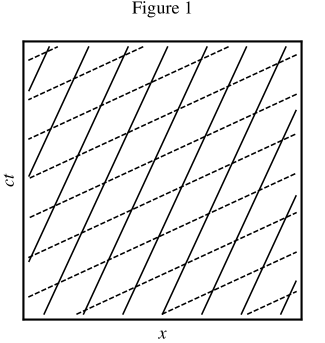
Figure 1: Contour plot of 1d inertial coordinates, $x^{\alpha^{\prime}}=(c\,t^{\prime},x^{\prime})$, as functions of the inertial coordinates, $x^{\alpha}=(c\,t,x)$, to which they are related via a Lorentz transformation [Eq. (5)]. The dashed lines are the contours of $t^{\prime}(c\,t,x)$. These represent “simultaneity submanifolds”—i.e., sets of spacetime events that occur simultaneously—for an inertial observer moving with the primed frame. The solid lines are the contours of $x^{\prime}(c\,t,x)$, any one of which could represent the trajectory of the moving inertial observer or particle, according to standard SR theory. Collectively, the solid lines constitute a relativistic quantum trajectory ensemble, describing a single relativistic particle undergoing quantum inertial motion.

More generally—i.e., for accelerated motion—the relativistic quantum trajectories and simultaneity submanifolds behave more along the lines indicated in Fig. 2. Unlike comoving frames,carroll ; weinberg ; rindler the simultaneity submanifolds of the present theory are curved. This is appropriate, given that the trajectories are also curved (albeit in the extrinsic rather than intrinsic sense). The curvature of the simultaneity submanifolds also enables them to avoid intersecting each other—thus also avoiding the problems of multiple reoccurences and incorrect time orderings that plague the comoving frame approach. Finally, the simultaneity submanifolds are everywhere orthogonal to the trajectories, and thus each submanifold consists only of spacelike separated events.

II.3 Ensemble time, and the generalized twin “paradox”

It should be noted that the ability to construct global simultaneity submanifolds is not automatic, but in fact, induces a slight constraint on the allowed form of $U^{\alpha}$. Using Frobenius’ theorem,carroll ; schutz and the fact that the $U^{\alpha}$ field is (presumed) smooth, it can be shown that only fields for which $h\,U^{\alpha}$ is four-curl-free (for some scalar field $h$) are permissible. (Technically, this is slightly more restrictive than the actual condition, but it is a sufficient condition that suits our purposes better). This condition implies that the four-velocity field is the normalized gradient of some scalar field $\lambda$:

$$U^{\alpha}=c{-\eta^{\alpha\beta}\,\partial_{\beta}\lambda\over\sqrt{-\eta^{\gamma\delta}\,\partial_{\gamma}\lambda\,\,\partial_{\delta}\lambda}},$$ (8)

where $\eta^{\alpha\beta}=\eta_{\alpha\beta}$ and $\partial_{\alpha}=\partial/\partial x^{\alpha}$ (and it is presumed that $\partial_{0}\lambda>0$).

The quantity $\lambda$ is a timelike parameter that we call an “ensemble time.” Actually, it is a full-fledged scalar field, and can therefore be interpreted as a global time coordinate. Eqs. (6) and (8) imply that the $\lambda=\rm{const}$ contours are the simultaneity submanifolds. The term “ensemble time” is therefore justified, as all members of the ensemble (i.e., all particle copies) agree that events corresponding to the same value of $\lambda$ occur simultaneously. The actual $\lambda$ value itself, however, is not uniquely defined. In general, any transformation of the form $\lambda\rightarrow{\lambda}^{\prime}={\lambda}^{\prime}(\lambda)$ yields a new ensemble time coordinate with the same contours, and which otherwise also satisfies Eq. (8). For the moment, we treat all such choices equally. Later, we will identify special candidates to serve as the “ensemble proper time,” $\lambda=\mathcal{T}$ (Secs. III.5 and V.3)—i.e., the ensemble analog of the usual single-path proper time, $\tau$.

Even for a path ensemble, it is straightforward—and often convenient—to construct a true proper time coordinate, $\tau$, as a scalar field on $M$. For each path in the ensemble, labeled by ${\bf C}$, one simply chooses a reference point $p$ at which $\tau$ is taken to be zero, and then integrates Eq. (2) along the path to find the value of $\tau$ at all other points. There is thus a freedom in the definition of the $\tau$ coordinate, associated with the particular choice of reference point $p$ for each path. This freedom corresponds to coordinate transformations of the form

$$\tau\rightarrow\tau^{\prime}=\tau^{\prime}(\tau,{\bf C})=\tau+\Delta({\bf C}),$$ (9)

where the shift, $\Delta({\bf C})$, varies across paths.

Although the $\tau$ coordinate is useful in its own right, note that any choice of $\tau$ is in general incompatible with any $\lambda$ coordinate of the form described above. In particular, for two different paths of a given ensemble, both starting at the same simultaneity submanifold ($\lambda$ contour) and ending at another, the elapsed ensemble time $\Delta\lambda$ is the same, but the elapsed proper times $\Delta\tau$ are (generally) different. Thus, $\tau$ per se cannot generally serve as a good ensemble time coordinate, $\lambda$.

The situation above is not problematic, and in fact, reflects nothing more than a generalized version of the well-known (but poorly named) twin “paradox.” The conventional twin paradox has one twin leaving the other at spacetime point $p_{0}$, only to rejoin him or her at a later point $p_{f}$, after having undergone accelerated motion. The accelerated trajectory of the second twin is necessary, in order that their paths may recross (the stay-at-home twin is presumed to undergo inertial motion). Since the starting point for both twins is in fact the same event $p_{0}$, there can be no question but that the departures occur simultaneously. Likewise, the reunion at $p_{f}$ is the same event for both twins, and must therefore also occur simultaneously. Nevertheless, we know that the elapsed proper times for the two twins are different, with the stay-at-home twin having aged (in some renditions, very significantly) more than his or her more adventurous sibling.

A similar situation characterizes our ensemble of paths—except that we now have a global definition of simultaneity, so that we can specify that two such paths begin “at the same moment” even if the initial spacetime events are different. Likewise, we can uniquely specify the simultaneous “end” of the two paths, as the points where these paths intersect a different $\lambda$ contour. The global property of the simultaneity submanifolds is indeed required, as any two paths within a given path ensemble never cross. Even though the two paths start and end simultaneously, the generalized twin paradox implies that there is no reason to expect the two elapsed $\Delta\tau$ values to be the same—and indeed they are not, in general. For the special case where all paths are moving inertially—i.e., for a “quantum inertial observer” (Fig. 1)—then the elapsed proper times for all paths are equivalent, and it is permissible in this instance to use $\tau$ as an ensemble time coordinate, $\lambda$. We thus make it a requirement of any reasonable definition for an ensemble proper time, $\mathcal{T}$, that it should reduce to the usual proper time, $\tau$, in the special case of a quantum inertial observer.

III General Coordinates and Probability

III.1 General (curvilinear) coordinates and natural coordinates

All of the equations of Sec. II have been presented in a way that is manifestly covariant, with respect to arbitrary coordinate transformations (diffeomorphisms). The general (or curvilinear) coordinate version of all such results is obtained by replacing the indices $\alpha$, $\beta$, etc. with $\mu$, $\nu$, etc., the inertial coordinates $x^{\alpha}$ with general coordinates $X^{\mu}$, and the Minkowski metric tensor with the generalized form,

$$g_{\mu\nu}=\eta_{\alpha\beta}\,{\partial x^{\alpha}\over\partial X^{\mu}}\,{\partial x^{\beta}\over\partial X^{\nu}}$$ (10)

Note also that in principle, all partial derivatives $\partial_{\alpha}$ that appear in Sec. II should be replaced with covariant derivatives,carroll ; weinberg denoted here as $\nabla_{\mu}$. However, these appear only in Eq. (8), where they are applied to a scalar invariant field ($\lambda$), for which it is well-known that $\nabla_{\mu}=\partial_{\mu}$ (in any coordinate system).

It is sometimes convenient to write Eq. (10) in matrix form,

$$\tilde{g}={\tilde{J}}^{T}\cdot\tilde{\eta}\cdot\tilde{J},$$ (11)

where ${J^{\alpha}}_{\!\mu}=\partial_{\mu}x^{\alpha}$ is the Jacobian matrix for the coordinate transformation $x^{\alpha}\rightarrow X^{\mu}$. We also define the inverse transform Jacobian matrix, $\tilde{K}$, as ${K^{\mu}}_{\!\alpha}=\partial_{\alpha}X^{\mu}$. Being true inverses of each other, ${J^{\alpha}}_{\!\mu}\,{K^{\mu}}_{\!\beta}=\delta^{\alpha}_{\beta}$, and ${K^{\mu}}_{\!\alpha}\,{J^{\alpha}}_{\!\nu}=\delta^{\mu}_{\nu}$, where in this context, $\delta$ is the Kronecker delta function.

Of all of the general coordinate systems that could be used to characterize our flat Minkowski spacetime manifold, $M$, obviously the global $x^{\alpha}$ inertial frame coordinates considered in Sec. II are a natural choice. However, for a given path ensemble, other natural choices also arise, based on quantities that we have already introduced. Let us hereby define a system of natural coordinates as the curvilinear choice,

$$X^{\mu}=(c\,\lambda,{\bf C})=(c\,\lambda,C^{i})=(c\,\lambda,C^{1},C^{2},C^{3}),$$ (12)

where $\lambda$ and $C^{i}$ are defined in Sec. II. In that section, these quantities were considered parameters; however, it is clear from the discussion therein that they can be promoted to full-fledged coordinates, forming a good coordinate system under the conditions discussed.

The physical meaning of the natural coordinates is such that the intersection of the contours of the three functions, $C^{i}(x^{\alpha})$, define the individual paths within the ensemble, whereas $\lambda$ itself describes the (ensemble) time evolution along a given path (see Figs. 2 and 3). Note that the introduction of a factor of $c$ into the definition of $X^{0}$ is consistent with the interpretation of $\lambda$ as a timelike coordinate. Likewise, the $C^{i}$ coordinates, which (as we have seen) can be used to label points on a given simultaneity submanifold, can be regarded as spacelike coordinates. That is not to say, however, that $\lambda$ must have units of time, and $C^{i}$ units of length. Rather, it is better to think of natural coordinates as being any choice that respects the natural division of $M$ into space and time that is induced by a given path ensemble (as described in Sec. II).

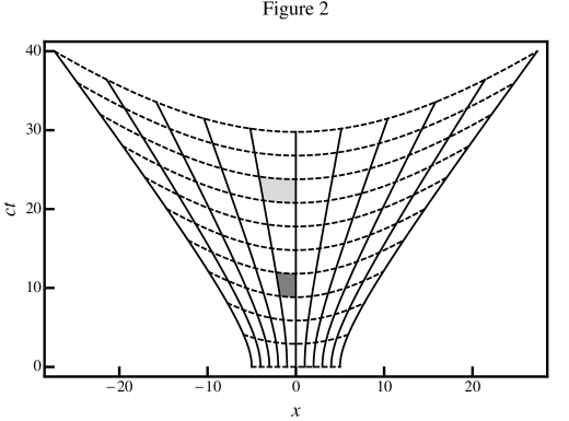
Figure 2: Quantum trajectories (solid curves) and simultaneity submanifolds (dashed curves) for the 1d $c\!\!=\!\!3$ relativistic Gaussian wavepacket of Sec. VI.3, as represented in the inertial coordinate frame, $x^{\alpha}=(c\,t,x)$. At $t\!\!=\!\!0$ (i.e., along the $x$ axis), all spacetime events occur simultaneously. The curvature of the simultaneity submanifolds at later times is an indication of relativistic dynamical effects, which are quite pronounced. The trajectories are everywhere normal (orthogonal) to the simultaneity submanifolds. The dark gray and light gray patches correspond to those in Fig. 3.

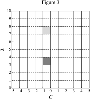
Figure 3: Quantum trajectories (solid curves) and simultaneity submanifolds (dashed curves) for the 1d $c\!\!=\!\!3$ relativistic Gaussian wavepacket of Sec. VI.3, as represented in a natural coordinate frame, $X^{\mu}=(c\,\lambda,C)$. All velocity and flux vectors point vertically (e.g., $U^{\mu}$), and all force vectors point horizontally (e.g., $f_{Q}^{\mu}$). The probability-length contained in each gray patch is identical to that of the corresponding patch in Fig. 2, and independent of the choice of $\lambda$ coordinate. This value is not the same for the light gray and dark gray patches, although these two patches do have the same value for the spatial scalar probability density, $f(C)$.

Further justification for this interpretation of the natural coordinates is provided by the fact that for any coordinate transformation of a form that respects this time/space division—i.e., the reparametrizations $\lambda\rightarrow{\lambda}^{\prime}={\lambda}^{\prime}(\lambda)$ and ${\bf C}\rightarrow{\bf C}^{\prime}={\bf C}^{\prime}({\bf C})$—the new coordinates, $X^{\mu^{\prime}}=(c\,\lambda^{\prime},{\bf C}^{\prime})$, are also seen to be natural coordinates, by the definition given above. For the moment, we treat all such choices equally. Later, however, after we have introduced suitable probabilistic structures and dynamical elements on $M$, we will find that a particular choice naturally emerges [i.e., $X^{\mu}=(c\,\mathcal{T},{\bf P})$].

An important feature of any set of natural coordinates—consistent with the above interpretation—is that the metric tensor $\tilde{g}$ be block-diagonal. Thus, $g_{0i}=g_{i0}=\eta_{\alpha\beta}{J^{\alpha}}_{\!0}{J^{\beta}}_{\!i}=0$, and so

$$\tilde{g}=\left(\matrix{g_{00}&{\bf 0}\cr{\bf 0}&\tilde{\gamma}}\right).$$ (13)

In Eq. (13) above, $\tilde{\gamma}$—the so-called “spatial metric”—represents the $3\times 3$ spatial block of the full metric tensor $\tilde{g}$. Natural coordinates are therefore orthogonal with respect to the division of space and time (although the spacelike coordinates $C^{i}$ are not necessarily orthogonal amongst themselves). This is a manifestation of the fact that the timelike and spacelike subspaces of the tangent vector spaces were constructed, by design, to be orthogonal to each other [Eq. (6)]. Note that reparametrizations of $\lambda$ do not affect $\tilde{\gamma}$, and reparametrizations of ${\bf C}$ do not affect $g_{00}$.

The block-diagonality assertion above is readily proven in terms of the inverse metric tensor,

$$g^{\mu\nu} = \eta^{\alpha\beta}{K^{\mu}}_{\!\alpha}{K^{\nu}}_{\!\beta}$$

$${\tilde{g}}^{-1} = {\tilde{K}}\cdot\tilde{\eta}\cdot{\tilde{K}}^{T}.$$ (14)

Note that ${K^{0}}_{\!\alpha}\propto\partial_{\alpha}\lambda$, whereas the contravariant vectors $\eta^{\alpha\beta}{K^{i}}_{\!\beta}$ describe displacements within the simultaneity submanifolds. Thus, from Eqs. (6) and (14), we have $g^{0i}=g^{i0}=0$, and the same must therefore be true for $\tilde{g}$ itself. Another useful set of relations to follow from the time/space orthogonality of the natural coordinates is

$$g^{00}={1\over g_{00}}=c^{2}\eta^{\alpha\beta}(\partial_{\alpha}\lambda)(\partial_{\beta}\lambda)=-\left({d\lambda\over d\tau}\right)^{2}.$$ (15)

The last equality relates the time-time component of the (inverse) metric tensor to $d\lambda/d\tau$, the local relation between ensemble and proper time (along a given trajectory/path).

Finally, we have a relation for the determinant of $\tilde{g}$, which will appear in various expressions. Following standard convention, we take

$$g=\det\tilde{g}=-(\det\tilde{J})^{2}=-J^{2}=-1/K^{2}$$ (16)

No absolute value is implied in Eq. (16) above; indeed, we see that $g$ must be negative. Equation (16) above is completely general. For natural coordinates, however, this reduces to

$$g=g_{00}\gamma,\qquad\rm{where}\quad\gamma=\det\tilde{\gamma}$$ (17)

(and $\gamma$ should not be confused with the index). It is clear from the previous definitions that $g_{00}<0$ and $\gamma>0$; thus, the -+++ signature of the inertial frame metric is retained, in keeping with our time/space interpretation of the natural coordinates.

III.2 Probability in 3d

Classical statistical mechanics, trajectory-based quantum mechanics, and relativistic hydrodynamics all include the notion of density fields that propagate through time and space.holland ; wyatt ; poirier10nowave ; poirier12nowaveJCP ; poirier12ODE ; carroll ; weinberg The densities are associated with corresponding flux vectors, that govern the local motion of fluid elements. Densities and their corresponding fluxes obey a continuity relationship, expressing the physical conservation law for a given quantity—be it energy/mass, charge, probability, or number of particles.

As we seek here to generalize the non-relativistic theory of quantum trajectory ensembles, and since the non-relativistic theory is mathematically equivalent to the TDSE, the conserved quantity in question can be taken to be probability. In the non-relativistic case, establishing the appropriate continuity equation is relatively straightforward—essentially because the time coordinate $t$ is uniquely determined. In the relativistic case, however, there are myriad probability-related quantities that can in principle be defined. One can construct both scalar and vector densities (current or flux four-vectors), as well as stress-energy-type tensors—all of which can be further subcategorized as to whether they exist on the full 4d spacetime, or only on submanifolds. In addition, whereas density quantities are generally not true invariants (i.e., with respect to general coordinate transformations),carroll ; weinberg one can often construct invariant versions of these quantities. To cut through the morass of possibilities, we apply the standard procedure of contemplating how such quantities, and the relationships among them, should transform under various coordinate transformations.

We also rely on the following assumption, borrowed from the non-relativistic theory:

• Postulate 1: Probability is conserved along quantum trajectories.

In the non-relativistic case, “probability” means the true, unitless, probability element—i.e., the (spatial) probability density times the (spatial) volume element, $\rho(t,{\bf x}(t))\,d^{3}x(t)$. Postulate 1 stipulates that along a given trajectory (i.e., for fixed $\bf C$), this quantity is independent of $t$. Under the coordinate transformation ${\bf x}\rightarrow{\bf C}$ (for fixed $t$), the probability density transforms as

$$\rho(t,{\bf x}(t))\,d^{3}x=f(t,{\bf C})\,d^{3}C,$$ (18)

because the probability element itself must be a scalar invariant. Since $\bf C$ and $d^{3}C$ are independent of $t$ along a trajectory, the probability conservation postulate therefore implies that $f(t,{\bf C})=f({\bf C})$ is itself independent of $t$. Thus, $f({\bf C})\,d^{3}C$ assigns a definite probability element to each trajectory in the ensemble, for all time.

We posit a similar situation in the relativistic case. Let $f({\bf C})$ be introduced as a probability density on $\bf C$ space—i.e., on the set of individual paths within a given ensemble. This density has units of $C^{-3}$, and is presumed to be normalized to unity:

$$\int\!f({\bf C})\,d^{3}C=1$$ (19)

The value of $f({\bf C})$ must be independent of the value of $\lambda$, in order to satisfy the probability conservation postulate—but equally importantly, it must be invariant of $\lambda$ reparametrizations, $\lambda\rightarrow\lambda^{\prime}(\lambda)$. The function $f({\bf C})$ can thus be “pulled back” to the individual simultaneity submanifolds on $M$,carroll ; weinberg but in no sense should it be regarded as a probability density on $M$ itself. We henceforth refer to $f({\bf C})$ as the “spatial scalar probability density” on ${\bf C}$.

The situation is exemplified by Fig. 3, which depicts the spacetime manifold $M$ as charted in a natural coordinate system. In this frame, individual paths appear as vertical lines, and simultaneity submanifolds (surfaces of constant $\lambda$) as horizontal lines. The evolution of ensemble time—technically, the $\lambda$-parametrized family of $M\rightarrow M$ diffeomorphisms generated by the $\lambda$ velocity vector field,

$$V^{\mu}={dX^{\mu}\over d\lambda}=(c,0,0,0)$$ (20)

—serves to advance the simultaneity submanifolds vertically through the spacetime $M$. Of course, the “rate” at which this occurs depends on the choice of ensemble time coordinate $\lambda$—which in turn affects the vertical length scale in Fig. 3, and the “thickness”, $c\,d\lambda$, of a four-volume element, $c\,d\lambda\,d^{3}C$. The changes in these quantities brought about by a reparametrization of $\lambda$ would in turn affect the values of any 4d density quantities on $M$. However, $\lambda$ reparametrization has no effect on the simultaneity submanifolds themselves, nor on the 3d quantities that live on these submanifolds, such as the spatial scalar probability density, $f({\bf C})$, and the spatial volume element, $d^{3}C$.

On the other hand, we of course demand that $f({\bf C})$ should transform as a probability density under reparametrization of the spatial coordinates, ${\bf C}\rightarrow{\bf C}^{\prime}$:

$$f^{\prime}({\bf C}^{\prime})d^{3}C^{\prime}=f({\bf C})d^{3}C\quad;\quad f^{\prime}({\bf C}^{\prime})=\sqrt{{\gamma^{\prime}\over\gamma}}f({\bf C})$$ (21)

Technically speaking, as a function of ${\bf C}$, $f({\bf C})$ is not a scalar invariant field, but a 3d scalar density of weight $W\!=\!-1$.

III.3 Probability and flux in 4d

As indicated, the 3d (spatial) $f({\bf C})$ density transforms in a well-prescribed way, under all coordinate transforms that preserve the natural coordinate structure. Our ultimate goal, however, is a fully covariant formalism, for which any choice of coordinates might in principle be used. We should therefore also consider the appropriate 4d scalar probability density (and the corresponding flux four-vector). A natural way to achieve this is through the use of the invariant form of the spatial scalar probability density—which is a true scalar invariant (weight $W\!\!=\!\!0$). We denote such invariant forms of density quantities with an asterisk superscript. The “spatial scalar invariant probability density” is thus found to be

$$f^{*}({\bf C})={f({\bf C})\over\sqrt{\gamma}},$$ (22)

as is evident from Eq. (21).

The advantage of working with true scalar invariants is that it is quite straightforward to pull back a scalar invariant function on $M$ to any submanifold of $M$, simply by restricting the domain of the function accordingly. In the present case, we would like to define a 4d scalar invariant probability density on all $M$, denoted $\rho^{*}(X^{\mu})$. What we have is a 3d spatial scalar invariant probability density $f^{*}$ defined on individual simultaneity submanifolds; but since the set of all such submanifolds foliate $M$, $f^{*}$ can be promoted to an actual scalar invariant function on $M$, i.e. $f^{*}(X^{\mu})$. It is therefore completely natural to define

$$\rho^{*}(X^{\mu})=f^{*}(X^{\mu})$$ (23)

in a generally covariant manner. The desired 4d scalar probability density (of weight $W\!=\!-1$) then becomes

$$\rho(X^{\mu})=\sqrt{|g|}\,\rho^{*}(X^{\mu})=\sqrt{{|g|\over\gamma}}\,f\left[{{\bf C}(X^{\mu})}\right]$$ (24)

Equation (24) above is the completely general covariant expression. In this context, however, it must be understood that $g$ refers to the completely general coordinates $X^{\mu}$, whereas $\gamma$ refers to the coordinates $\bf C$. In the special case where $X^{\mu}=(c\,\lambda,{\bf C})$ is taken to be the natural coordinate frame itself, then Eq. (24) reduces to

$$\rho(X^{\mu})=\sqrt{-g_{00}}\ f({\bf C})=\left({d\tau\over d\lambda}\right)f({\bf C}).$$ (25)

In any event, $\rho(X^{\mu})$ behaves as a true 4d scalar density should; the element $\rho(X^{\mu})\,d^{4}X$ is a scalar invariant. This element is not unitless, however; it has units of length, as the invariant form $\rho^{*}$ has units of length^-3.

From the scalar probability density $\rho(X^{\mu})$, we wish to construct a flux four-vector, $j^{\mu}$, such that

$$j_{\mu}\,j^{\mu}=g_{\mu\nu}\,j^{\nu}j^{\mu}=-c^{2}\rho^{2}.$$ (26)

Intuition (e.g., from electromagnetic current) suggests that $j^{\mu}$ should transform as a contravariant four-vector, which would make $\rho$ a scalar invariant. In SR, this is completely correct, in the sense that $\rho^{\prime}(x^{\alpha^{\prime}})=\rho(x^{\alpha})$ is unaltered under Lorentz transformations, because the volume element $d^{4}x^{\prime}=d^{4}x$ is unchanged. Thus, $j^{\mu}$ indeed transforms as a four-vector under Eq. (5). In the completely general context however, incorporating transformations to curvilinear coordinate frames, one finds that $\rho$ and $j^{\mu}$ should transform, respectively, as scalar and contravariant vector densities, of weight $W\!=\!-1$. This distinction is quite critical from the perspective of the covariant continuity equation (to be defined shortly).

From Eqs. (3) and (26), and the requisite transformation properties, the desired flux quantity is evidently

$$j^{\mu}=\rho(X^{\mu})\,U^{\mu}=f({\bf C})\,V^{\mu},$$ (27)

where the first equality is generally true, and the second holds [from Eqs. (20) and (25)] in a natural coordinate frame.

III.4 Covariant continuity

Next, we derive a continuity equation in a natural coordinate frame. We expect this to take the form of a vanishing four-divergence of $j^{\mu}$, i.e.

$$\partial_{\mu}\,j^{\mu}=0$$ (28)

From Eqs. (20) and (27), the flux in a natural coordinate frame is given by $j^{\mu}=(c\,f({\bf C}),0,0,0)$, for which Eq. (28) is clearly satisfied, by virtue of the probability conservation postulate.

Is Eq. (28) also true for general coordinates? Since derivatives of vector quantities are involved, ordinarily, one would have to replace the partial derivatives in Eq. (28) with covariant derivatives, in order to obtain a generally covariant expression. However, for the special case of a contravariant vector density with weight $W\!=\!-1$ (or a covariant vector density with weight $W\!\!=\!\!+1$) it turns out that the covariant four-divergence is equal to the usual (partial derivative) four-divergence. Thus, $\partial_{\mu}\,j^{\mu}=\nabla_{\mu}\,j^{\mu}$ holds in all coordinate frames, and therefore, so does Eq. (28). We take this to be the covariant continuity equation.

The four-divergence property described above can be proven as follows. Let $j^{\mu}$ be a contravariant vector density of weight $W\!=\!-1$. The standard expression for the covariant derivative is

$$\nabla_{\nu}\,j^{\mu}=\partial_{\nu}\,j^{\mu}+\Gamma^{\mu}_{\nu\kappa}\,j^{\kappa}-\Gamma^{\kappa}_{\nu\kappa}\,j^{\mu},$$ (29)

where the $\Gamma^{\mu}_{\nu\kappa}$ are the famous Christoffel symbols,carroll ; weinberg defining the (metric compatible) connection:

$$\Gamma^{\mu}_{\nu\kappa}={1\over 2}g^{\mu\sigma}(\partial_{\nu}g_{\kappa\sigma}+\partial_{\kappa}g_{\sigma\nu}-\partial_{\sigma}g_{\nu\kappa})$$ (30)

To obtain the covariant divergence from Eq. (29), $\nu$ is set equal to $\mu$, which then becomes a dummy index that is summed over (Einstein notation). By the symmetry of the Christoffel symbols with respect to their lower indices, the second and third terms in Eq. (29) then cancel, leaving the desired equality.

The covariant continuity equation is easiest to interpret in a natural coordinate frame. Here, the $j^{\mu}$ vector field is “vertical” (Fig. 3), and simply describes how probability density is carried along under the action of the $V^{\mu}$ velocity field. It is important to note that it is the spatial scalar probability density, $f({\bf C})$, that is conserved in this sense, not the scalar probability density $\rho(X^{\mu})$ per se. To within a constant factor of $c$, the former is just the zeroth component of the flux four-vector, $j^{0}$, in a natural coordinate frame. More generally, i.e. in an arbitrary coordinate system, it is $(j^{0}/c)$ that we ordinarily think of as the “probability density”. In particular, if $X^{\mu}$ is any coordinate system for which $X^{0}$ and $X^{i}$ are orthogonal, then Eq. (28) and the generalized Stokes theoremcarroll imply that

$$\int j^{0}(X^{\mu})\,dX^{1}dX^{2}dX^{3}={\rm const,}\qquad{\rm for\ all}\,\,X^{0}$$ (31)

[provided $j^{0}(X^{\mu})$ vanishes asymptotically].

Note that the orthogonal condition above is not the same as the natural coordinate condition, and is in fact far less restrictive. For instance (and in addition to any natural coordinate frame) it includes any inertial coordinate frame, $X^{\mu}=x^{\alpha}$, in which case Eqs. (28) and (31) reduce to the usual SR forms. The inertial frame forms of the density and flux quantities bear further discussion. From Eq. (24), we find that

$$\rho(x^{\alpha})=\rho^{*}(x^{\alpha})={f\!\left[{{\bf C}(x^{\alpha})}\right]\over\sqrt{\gamma}}.$$ (32)

Likewise, from Eqs. (25) and (27), we obtain

$$j^{\alpha} = {f\!\left[{{\bf C}}\right]\over\sqrt{\gamma}}\,U^{\alpha}=c\,{f\!\left[{{\bf C}}\right]\over\sqrt{-g_{00}\gamma}}\,{J^{\alpha}}_{\!0}$$

$$\quad j^{0} = c\,{f\!\left[{{\bf C}}\right]\over\sqrt{\gamma}}\,{dt\over d\tau}$$ (33)

Clearly, $\rho(x^{\alpha})$ and $(j^{\alpha}/c)$ both have units of length^-3, as they should. Note that $g_{00}$, $\gamma$, and ${J^{\alpha}}_{\!0}$ refer to the natural coordinate frame.

III.5 Uniformizing natural coordinates

Let us return to a natural coordinate frame, and consider the ensemble time evolution, as indicated in Figs. 2 and 3. Although the probability element $\rho(X^{\mu})\,d^{4}X$ is not conserved along trajectories, it is invariant. Thus, the probability-length contained within the dark gray patches in Fig. 2 and Fig. 3 is the same, and the probability-length within the light gray patches in Fig. 2 and Fig. 3 is the same, but the value for the dark gray patches is not the same as for the light gray patches. Fundamentally, this is because $\lambda$ and $\tau$ are generally incompatible, and so $d\tau/d\lambda$ must vary across $M$. Put another way, a reparametrization of $\lambda$ could expand the vertical scale of the light gray patches without necessarily changing that of the dark gray patches, which has a corresponding effect on the $\rho$ values. Clearly, $\rho$ cannot be conserved for a general choice of ensemble time, $\lambda$.

Nevertheless, it would be nice if we could define a “proper-time like” reparametrization of $\lambda$, for which $\rho(X^{\mu})$ was as close to being conserved as possible. The best we can manage along these lines is to choose a $\lambda$ such that the spatial integral of $\rho(X^{\mu})$, i.e.

$$\int\!\rho(X^{\mu})\,d^{3}C=\int{d\tau\over d\lambda}\,f({\bf C})\,d^{3}C$$ (34)

is conserved over time. We can therefore define, as an ensemble proper time, $\mathcal{T}$, that choice of ensemble time $\lambda$ for which

$$\int\!{d\tau\over d\mathcal{T}}\,f({\bf C})\,d^{3}C=1,\qquad{\rm for\ all}\,\,\mathcal{T}.$$ (35)

The interpretation of Eq. (35) is straightforward. By multiplying both sides by $d\mathcal{T}$, we see that, at any time $\mathcal{T}$, the interval $d\mathcal{T}$ is just the path ensemble average of the proper time interval $d\tau$. If the $d\tau$ intervals happen to be the same for all paths in the ensemble at a given $\mathcal{T}$, then $d\mathcal{T}=d\tau$ at that time. If this is true at all times, then $\mathcal{T}=\tau$—as describes the special case of quantum inertial observers. In general though, the $d\tau$ values differ across the ensemble, and so $d\mathcal{T}$ is obtained as the probability-weighted average of the $d\tau$ values for the individual paths. Note that for a given path ensemble, the $\mathcal{T}$ coordinate as specified here is uniquely defined, to within an overall additive constant.

As reasonable as the above prescription may appear, Eq. (35) is not the most natural choice for an ensemble proper time, $\mathcal{T}$; that choice will be introduced in Sec. V.3. For one thing, even with Eq. (35), the probability-length of the dark gray patches in Figs. 2 and 3 is still not equal to that of the light gray patches—although the spatial integrals across the simultaneity submanifolds are now equal. The ensemble proper time as defined above can be regarded as a “uniformizing coordinate,” in the sense that it does the best possible job of spreading out the scalar probability density, $\rho(X^{\mu})$, uniformly throughout (ensemble) time.

One might also consider a similar reparametrization of the (natural) spatial coordinates, ${\bf C}$. Here, it is possible to perfectly uniformize the probability distribution $f({\bf C})$, and in fact, exactly this procedure has been used in the previous non-relativistic work.poirier12nowaveJCP We hereby denote such a uniformizing choice of spatial coordinates for $\bf C$ as $\bf C\!=\!P$, defined such that

$$f({\bf P})=1.$$ (36)

For a single spatial dimension, the $P$ coordinate is uniquely determined, apart from an additive constant (which fixes the range of allowed $P$ values); it can be interpreted as the total (integrated) probability that exists to the left of a given path in the ensemble (hence the nomenclature “$P$,” often used in such contexts). In higher dimensional spaces, the $\bf P$ coordinates are also uniquely determined—apart from (spatial) volume-preserving diffeomorphisms.

With $\mathcal{T}$ taken to be any ensemble proper time [e.g., either that of Eq. (35) or of Sec. V.3], we regard $X^{\mu}=(c\,\mathcal{T},{\bf P})$ to comprise a set of “uniformizing natural coordinates,” in terms of which $\mathcal{T}$ has units of time, ${\bf P}$ is unitless, $f({\bf P})=1$ is unitless, and $\rho(X^{\mu})=(d\tau/d\mathcal{T})f/\sqrt{\gamma}$ has units of length^-3 (as for the inertial frame case).

IV Dynamical Considerations

We now have many of the elements in place that we need to develop a trajectory-based theory of relativistic quantum dynamics. However, there are still a few more issues, dynamical in nature, that must first be addressed. In the first two subsections below, we consider single-trajectory classical dynamics, both non-relativistic and relativistic. Even in this context, there are certain subtle aspects that turn out to have extremely important ramifications for the relativistic quantum case. In the third subsection below, we consider the trajectory-based non-relativistic quantum theory, presenting some key results from earlier work, and setting the stage for addressing quantum effects in the relativistic context.

IV.1 Classical dynamical considerations

Consider a single, non-relativistic classical particle. The dynamics are described by the trajectory, $x^{l}(t)$. The velocity vector is ${\dot{x}}^{l}=dx^{l}/dt$, and the non-relativistic classical equation of motion is

$$m{\ddot{x}}^{l}=-{\partial V(t,{\bf x})\over\partial x^{l}}=f^{l},$$ (37)

where $V(t,{\bf x})$ is the potential energy field, and $f^{l}$ is the force vector. Note that we are considering the general, nonconservative case where $V$ may depend on $t$ as well as ${\bf x}$. The reason is that we wish to adopt a 4d spacetime viewpoint, even in this non-relativistic context. We therefore continue to use notation such as “$x^{\alpha}$” and “$g_{\alpha\beta}$,” mostly without ambiguity. Thus, for example, the Euclidean metric, $g_{\alpha\beta}=\delta_{\alpha\beta}$ is presumed.

From this 4d vantage, a striking feature of Eq. (37) is that the force vector does not include a time component, even when $V$ depends on $t$. In other words, the dynamical equations do not make use of what would be the entire force four-vector, $f^{\alpha}=f_{\alpha}=\partial_{\alpha}V$, but only the spatial components of this vector—i.e., the projection onto the (non-relativistic) simultaneity submanifold (just 3d space itself, ${\bf x}$). If the time component were used, it would lead to an additional dynamical equation of the form

$$m{\ddot{t}}=f^{0}\propto-{\partial V\over\partial t},$$ (38)

which is manifestly incorrect for time-dependent potentials, because ${\ddot{t}}=d{\dot{t}}/dt=d(1)/dt=0$.

From a physical standpoint, the restriction to just the spatial components of the force vector is not surprising. Suppose that the partial time derivative of $V(t,{\bf x})$ were employed in the determination of the dynamical force. That would mean that this force, which drives the future time evolution of the particle, would itself depend on the future states of that particle—a highly untenable situation vis-à-vis causality, which can be reasonably dismissed. Of course, time reversibility implies that the force must also be independent of the past state of the particle, which leaves only the present. In this manner, we are led to:

• Postulate 2: All force vectors, together with the quantities used in their construction, must “live” on the simultaneity submanifolds.

The meaning of this statement will be made more precise as we go along. In any case, we take Postulate 2 as a necessary condition for any viable physical theory—at least for particles with mass, in the context of non-relativistic or relativistic classical or quantum mechanics. As shown above, it certainly holds for non-relativistic classical particles.

It also holds for relativistic classical particles, as we now demonstrate. Of course, it is not possible to define a global simultaneity submanifold from a single relativistic trajectory, $x^{\alpha}(\tau)$. All that is required for the present purpose, though, is a local specification of simultaneity, which we do in fact have. As discussed in Sec. II, this is found—for a given point $p$—in the orthogonal subspace of $T_{p}$ that is orthogonal to $U^{\alpha}$ at $p$. According to Postulate 2, the relativistic force vector $f^{\alpha}$ must belong to this orthogonal subspace. That this is the case can be shown using the relativistic classical equation of motion:

$$m{d^{2}x^{\alpha}\over d\tau^{2}}=m{dU^{\alpha}\over d\tau}=f^{\alpha}$$ (39)

(note that we are still working in an inertial frame). From Eqs. (3) and (39),

$${m\over 2}\,{d(\eta_{\alpha\beta}\,U^{\alpha}U^{\beta})\over d\tau}=\eta_{\alpha\beta}\,U^{\alpha}f^{\beta}=0.$$ (40)

Thus, indeed, $f^{\alpha}$ belongs to the orthogonal subspace, and hence points along the simultaneity submanifold.

Let us pause to consider the ramifications of Eq. (40). Since the orthogonal subspace at a given point $p$ depends on the trajectory, this implies that $f^{\beta}$ itself must also depend on the trajectory at $p$—i.e., not just on the point itself. Thus, for example, a relativistic force vector can never be simply the gradient of some scalar invariant potential: $f^{\alpha}\neq-\eta^{\alpha\beta}\partial_{\beta}\Phi$. On the other hand, one simple way that Eq. (40) can be achieved is by taking $f^{\alpha}$ to be the product of an antisymmetric tensor and $U^{\alpha}$. This is the general form for the relativistic force that ensues when the Lagrangian includes a term that is the scalar product of $U^{\alpha}$ and some four-vector field. The classic example is the vector potential, $A_{\alpha}$, of electromagnetic theory, for which the resultant antisymmetric tensor, $F_{\alpha\beta}$, is the electromagnetic field strength tensor. Thus, the “velocity-dependent” nature of a relativistic force field—well-known in the electromagnetic context—is seen to be a general requirement arising from Postulate 2.

Note that, whereas $f^{\alpha}$ does indeed belong to the orthogonal subspace of $T_{p}$, the same cannot be said for $A_{\alpha}$ and $U^{\alpha}$—despite the fact that these are clearly “elements used in the construction” of $f^{\alpha}$. Postulate 2 can still be regarded to be satisfied—albeit in a weaker sense than for $f^{\alpha}$ itself—because the $A_{\alpha}$ and $U^{\alpha}$ vectors belong to the tangent space $T_{p}$ for the point $p$ itself, and not some other point. Thus, in that sense, these vector quantities belong to the simultaneity submanifold. The main point, though, is that $f^{\alpha}$ should in no sense depend on quantities associated with the future (or past) particle states. Taking $p$ and $U^{\alpha}$ together as constituting the local state of the particle, then the determination of $f^{\alpha}$ at $p$ should not depend on future or past values for these quantities, neither explicitly nor implicitly.

Technically speaking, it is the $F_{\alpha\beta}$ tensor, rather than $A_{\alpha}$ itself, that is used in the construction of $f^{\alpha}$. As it happens, the $F_{\alpha\beta}$ tensor does depend on future particle states, because this quantity is obtained from all partial derivatives of $A_{\alpha}$. Thus, it is not only $A_{\alpha}$ at the point $p$ itself that is consulted, but also, the value of $A_{\alpha}$ at nearby points, displaced from $p$ in all four spacetime directions. This situation might appear to violate Postulate 2, but in fact, it does not. The reason is that the full $F_{\alpha\beta}$ tensor is not actually required to construct $f^{\alpha}$—only that portion of the tensor that is projected onto the local simultaneity submanifold is used. Consequently, although $A_{\alpha}$ values at points other than $p$ are required, these points occur simultaneously with $p$, lying neither in its past nor its future, and so Postulate 2 is indeed satisfied. Similar arguments will prove relevant, also, for quantum force fields, although these arise in an altogether different manner.

A more precise statement of Postulate 2 also requires a clearer specification of the dynamical “evolution coordinate,” denoted $\xi$. Under arbitrary reparametrizations, $\xi\rightarrow\xi^{\prime}(\xi)$, the forms of Eqs. (37) and (39) are not preserved, and—depending on interpretation—“time” components of the resultant force vectors do in fact arise. However, these should be properly regarded as fictitious. The fact is that the metric tensor, together with the local simultaneity submanifolds, give rise to a natural local choice for $\xi$, in terms of which Postulate 2 may be expected to hold. This choice is such that $\xi=\rm{const}$ within the simultaneity submanifold, and $d\xi/ds=\rm{const}$ for displacements perpendicular to the simultaneity submanifold (where $ds^{2}$ is the line element, defined in Sec. II.1). This specification of the evolution coordinate $\xi$ may be applied to both the non-relativistic and relativistic cases considered above—giving rise to $\xi=t$ and $\xi=\tau$, respectively (more generally, $\xi$ may also include affine transformations of the above forms). With these choices for $\xi$, we have already seen that Postulate 2 holds for both non-relativistic and relativistic classical mechanics.

IV.2 Arbitrary time reparametrizations, as applied to classical electromagnetism

As the canonical example of a relativistic classical force field with the above velocity-dependent form, we consider the case of electromagnetism in some detail. This will turn out to be of particular benefit for the development of relativistic quantum force fields, in at least two ways. First, it provides an understanding of how potential energy contributions, in general, should enter into the relativistic Lagrangian. The second benefit emerges from a reworking of the electromagnetic example in terms of an arbitrary time reparametrization, i.e. $\tau\rightarrow\lambda(\tau)$, which is not usually seen in standard treatments. In the electromagnetic context, this introduces unnecessary complexity, but it provides important insight into how to handle the relativistic quantum case—for which, as we have seen in Sec. III, ensemble time $\lambda$ and proper time $\tau$ are incompatible.

Let us start with the simplest case of a free particle. Let $x^{\alpha}(\lambda)$ denote an arbitrary timelike path, described by the arbitrary parameter $\lambda$. For fixed endpoints, the solution trajectory is that which maximizes the elapsed proper time, $\Delta\tau$—i.e., it is a geodesic. From Eq. (2), the elapsed proper time along any path is given by

$$\Delta\tau=\int\!\left({d\tau\over d\lambda}\right)d\lambda=\int\!\sqrt{-{1\over c^{2}}\,\eta_{\alpha\beta}\,{dx^{\alpha}\over d\lambda}\,{dx^{\beta}\over d\lambda}}\,d\lambda.$$ (41)

One standard choice for $\lambda$ is the proper time, $\tau$, itself. Making this choice, and multiplying Eq. (41) by the negative rest energy, $-mc^{2}$, the maximization of $\Delta\tau$ is converted into the equivalent minimization of the action,

$$S=\int\!L\!\left[{x^{\alpha}_{\tau}}\right]d\tau=\int(-mc^{2})\sqrt{-{1\over c^{2}}\,\eta_{\alpha\beta}\,x^{\alpha}_{\tau}\,x^{\beta}_{\tau}}\,d\tau,$$ (42)

where $x^{\alpha}_{\tau}$ denotes $dx^{\alpha}/d\tau=U^{\alpha}$, and $L[x^{\alpha}_{\tau}]$ is the Lagrangian for the parameter choice, $\lambda=\tau$.

Regardless of the particular choice of $\lambda$, the form on the right hand side of Eq. (41) should be used in the Lagrangian. This is because it exhibits explicit dependences on $x^{\alpha}_{\lambda}=dx^{\alpha}/d\lambda=V^{\alpha}$, and thus gives rise to an Euler-Lagrange ordinary differential equation (ODE) for the solution trajectory, $x^{\alpha}(\lambda)$, in terms of the first and second $\lambda$ derivatives. Specifically, action minimization leads to the following Euler-Lagrange form:

$${\partial L\over\partial x^{\alpha}}-{d\over d\lambda}\left({{\partial L\over\partial x^{\alpha}_{\lambda}}}\right)=0$$ (43)

For the standard choice $\lambda=\tau$, and the flat Minkowski spacetime metric presumed here, the result is Eq. (39) (with $f^{\alpha}=0$). For curved spacetime manifolds, or flat manifolds described via curvilinear coordinates, $X^{\mu}$, taking $\lambda=\tau$ leads to the standard geodesic equation,carroll ; weinberg

$$X^{\mu}_{\tau\tau}+\Gamma^{\mu}_{\nu\kappa}\,X^{\nu}_{\tau}\,X^{\kappa}_{\tau}=0.$$ (44)

To a large extent, the above procedure is straightforward because of the presumed $\lambda=\tau$ form, and the constraint that that induces. Even in this context, there are some ambiguities that can arise. Specifically, the square root quantity in Eq. (42) is necessarily equal to one. Why not simply replace this expression with $1$, or otherwise multiply or divide $L[x^{\alpha}_{\tau}]$ by as many such square root factors as we wish? Likewise, incorporating the $\lambda=\tau$ constraint explicitly into the optimization using the theory of Lagrange multipliers, one should be able to add or subtract additional terms of this form. Even for the free particle case, this can lead to trouble—e.g., to $S=\int(-mc^{2})\,d\tau$, which is useless from the point of view of generating any ODE for $x^{\alpha}(\tau)$, much less the correct one. The situation is even more delicate, however, when a potential energy contribution is introduced into the Lagrangian.

Consider, then, the standard form of the Lagrangian (in $\tau$) for a single relativistic particle with charge $q$, acted on by the electromagnetic vector potential, $A_{\alpha}$:

$$L\!\left[{x^{\alpha},x^{\alpha}_{\tau}}\right]=(-mc^{2})\sqrt{-{1\over c^{2}}\,\eta_{\alpha\beta}\,dx^{\alpha}_{\tau}\,dx^{\beta}_{\tau}}+{q\over c}\,x^{\alpha}_{\tau}\,A_{\alpha}$$ (45)

The potential energy contribution [i.e., the second term on the right hand side of Eq. (45)] introduces an explicit Lagrangian dependence on the coordinates $x^{\alpha}$, through the $A_{\alpha}$ vector field. The Lagrangian form of Eq. (45) leads via Eq. (43) to the correct electromagnetic ODE—i.e., Eq. (39), with

$$f^{\alpha}={q\over c}\,\eta^{\alpha\beta}F_{\beta\gamma}\,x^{\gamma}_{\tau}\quad{\rm and}\quad F_{\beta\gamma}=\partial_{\beta}A_{\gamma}-\partial_{\gamma}A_{\beta}.$$ (46)

The above derivation requires explicit substitution of the Eq. (2) equality—but only after the Lagrangian partial derivatives of Eq. (43) have been applied. Note that the one factor of the square root quantity in the first term of Eq. (45) is necessary to generate the kinetic energy contribution in the resultant equation of motion. The potential energy term of the Lagrangian does not include this square root factor; if it did, the resultant ODE would be incorrect. Likewise, any additional factors of the square root quantity in the first (kinetic) term of $L$ would also lead to incorrect ODEs.

We will apply these findings to relativistic quantum force fields, but first we must also consider the general $\lambda$ case explicitly. This can be regarded in terms of the coordinate transformation, $\tau\rightarrow\lambda(\tau)$. Since the action, $S$, must be a scalar invariant, $L$ must transform as a scalar density of weight $W\!=\!-1$—leading at once to the following form for the Lagrangian in $\lambda$:

$$L\!\left[{x^{\alpha},x^{\alpha}_{\lambda}}\right]=(-mc^{2})\sqrt{-{1\over c^{2}}\,\eta_{\alpha\beta}\,x^{\alpha}_{\lambda}\,x^{\beta}_{\lambda}}+{q\over c}\,x^{\alpha}_{\lambda}\,A_{\alpha}$$ (47)

At this point, we must distinguish between two possibilities: the case where the explicit relation $\lambda(\tau)$ is known a priori, vs. the case where it is not. In the former case, $\lambda(\tau)$ implies an explicit constraint, analogous to (but more complicated than) that of Eq. (2) for $\lambda=\tau$. One can therefore apply a procedure similar to that used for $\lambda=\tau$—i.e., the explicit constraint is invoked only after the Lagrangian partial derivatives have been evaluated. The resultant ODE is the general-$\lambda$ version of Eq. (39), i.e.,

$$m\,x^{\alpha}_{\lambda\lambda}=\tau_{\lambda}^{2}\,f^{\alpha}+m\,{\tau_{\lambda\lambda}\over\tau_{\lambda}}\,x^{\alpha}_{\lambda},$$ (48)

where $\tau_{\lambda}=d\tau/d\lambda$, and $f^{\alpha}$ is from Eq. (46). That this form is correct may be readily verified—e.g., for the choice $\lambda=t=x^{0}/c$, in terms of which the classical electromagnetic equations of motion are very well known.

Let us now imagine—as is the case in the quantum context—that the relation $\lambda(\tau)$ [or the inverse, $\tau(\lambda)$] is not necessarily known a priori. This situation is evidently problematic, from the perspective of the $\lambda$ evolution of Eq. (48). At the initial time, it is straightforward enough to specify initial values for $\tau_{\lambda}$ and $\tau_{\lambda\lambda}$—or equivalently, $\lambda_{\tau}$ and $\lambda_{\tau\tau}$. However, there are many functions $\lambda(\tau)$ that share the same initial conditions, any one of which might in principle be legitimately used; so how does the ODE “know” which choice to make, during the course of the propagation, if this is not already specified a priori?

To address this question, the only recourse is to use the generic relation for $\tau_{\lambda}$, as implied by Eq. (41). Substituting this form into Eq. (48)—or equivalently, deriving the Euler-Lagrange ODE from Eq. (47) without applying any explicit constraint—one obtains

$$m\,x^{\alpha}_{\lambda\lambda}=\left(-{1\over c^{2}}\,\eta_{\beta\gamma}\,x^{\beta}_{\lambda}\,x^{\gamma}_{\lambda}\right)f^{\alpha},$$ (49)

which is equivalent to Eq. (48), but without the last term. Thus, $\tau_{\lambda\lambda}=\lambda_{\tau\tau}=0$, or $\lambda(\tau)=A\tau+B$. In other words, this procedure automatically picks out an affine relation for $\lambda(\tau)$, if no relation is specified a priori. (The values of the constants $A$ and $B$ are uniquely determined from the initial values for $\lambda$ and $\lambda_{\tau}$, which are arbitrary).

All of the above is perfectly consistent—albeit unnecessarily complicated—in the context of relativistic electrodynamics. The situation does not bode so well, however, for the relativistic quantum dynamical case. Here, we know that $\lambda$ and $\tau$ do not satisfy any global functional relationship of the form $\lambda=\lambda(\tau)$—much less an affine relation. Locally—and along a single given trajectory of the ensemble—such a relation can of course be established, although it is not necessarily known a priori, even in this context. All of this suggests that, in the quantum case, we must proceed with caution.

IV.3 Non-relativistic quantum dynamical considerations

The trajectory-based formulation for non-relativistic quantum dynamics is, by this point, fairly well established.bouda03 ; holland05 ; poirier10nowave ; holland10 ; poirier11nowaveCCP6 ; poirier12nowaveJCP ; poirier12ODE Here, we review only those features that are most relevant for the relativistic generalization of Sec. V. Also, whereas our previous work has expressed the requisite quantities in terms of the Jacobian matrices, ${J^{l}}_{\!i}$ and ${K^{i}}_{\!l}$, here, we adopt a tensorial, generally covariant viewpoint, relying on the (spatial) metric tensor $\gamma_{ij}$, and its determinant, $\gamma$.

The non-relativistic formulation makes use of a spatial coordinate transformation from $x^{l}$ to $C^{i}$, for which the time coordinate, $t$, is unaffected. As in the relativistic case, the $C^{i}$ serve as trajectory labeling coordinates for a trajectory (or path) ensemble. As discussed in Sec. IV.1, the simultaneity submanifolds are defined by surfaces of constant $t$ in the 4d non-relativistic spacetime manifold, $M$. The $x^{l}\rightarrow C^{i}$ transformation is thus parametrized by $t$, with a complete solution trajectory ensemble taking the form $x^{l}(t,{\bf C})$. In the $x^{l}$ coordinate frame, the metric tensor is presumed to be the usual Euclidean one, $\delta_{lm}$, whereas in the $C^{i}$ coordinates, the metric tensor is denoted $\gamma_{ij}$. The latter is a function of both space $({\bf C})$ and time ($t$).

As in the relativistic case, Postulate 1 is presumed (or, it can be regarded as a logical consequence of Bohmian mechanicsmadelung26 ; bohm52a ; bohm52b ; holland ; wyatt ; durr92 ; berndl95 ). The scalar probability density in ${\bf C}$ space, $f({\bf C})$, is thus independent of $t$, and Eq. (19) is presumed to hold. From Eq. (18), we have

$$R(t,{\bf x})={f({\bf C})^{1/2}\over\gamma^{1/4}},$$ (50)

where $R(t,{\bf x})=\rho(t,{\bf x})^{1/2}$ is the usual wavefunction amplitude, $|\Psi|$—i.e., the square root of the usual spatial probability density, $\rho(t,{\bf x})=\Psi^{*}\Psi$. The latter is a 3d density akin to $j^{0}/c$ from Sec. III.4, but in the non-relativistic context, it can also be interpreted as the 4d scalar probability density of Sec. III.3.

We expect a scalar invariant action, $S$, of the form

$$S = \int\!\mathcal{L}[x^{l},{\dot{x}}^{l},\partial_{i}x^{l},\ldots]\,d^{3}C\,dt$$ (51)

$$= \int\!L[x^{l},{\dot{x}}^{l},\partial_{i}x^{l},\ldots]f({\bf C})\,d^{3}C\,dt,$$

where ${\dot{x}}^{l}=(\partial x^{l}/\partial t)|{\bf C}$ and $\partial_{i}=\partial/\partial C^{i}$. The quantity $\mathcal{L}$ is the Lagrangian density (a spatial scalar density of weight $W\!=\!-1$), whereas $L$ is a scalar invariant quantity (with units of energy) that we refer to simply as “the Lagrangian” (although technically, that term should be applied to the $d^{3}C$ integral of $\mathcal{L}$.) The Lagrangian is a true scalar invariant (weight $W\!=\!0$). In non-relativistic quantum mechanics, it takes the form

$$L = {1\over 2}m\,\delta_{lm}\,{\dot{x}}^{l}\,{\dot{x}}^{m}-V({\bf x})-$$

$${\hbar^{2}\over 8m}\left[{f({\bf C})\over\gamma^{1/2}}\right]^{-2}\!\!\gamma^{ij}\,\partial_{i}\!\!\left[{f({\bf C})\over\gamma^{1/2}}\right]\partial_{j}\!\!\left[{f({\bf C})\over\gamma^{1/2}}\right].$$

The metric tensor $\tilde{\gamma}$ depends explicitly on the $\partial_{i}x^{l}$; the specific Lagrangian of Eq. (IV.3) is therefore second order in the $C^{i}$ derivatives of $x^{l}$ (although an alternate, higher order choice of $L$ will also be considered).

The last term in Eq. (IV.3) above is the (scalar invariant) quantum contribution to the Lagrangian, denoted $-L_{Q}$. This term accounts for all interaction or “communication” across trajectories—and hence, for all quantum dynamical effects.holland05 ; holland10 ; poirier12nowaveJCP It can be expressed in a variety of ways, with the Eq. (IV.3) form above being particularly explicit. Note that Eqs. (22), (32), and (50) imply that the quantity in square brackets can be interpreted as the spatial scalar invariant probability density, $f^{*}$—or equivalently, as the usual $\rho(t,{\bf x})=R(t,{\bf x})^{2}$. Because $f^{*}$ is a scalar invariant, the partial derivatives $\partial_{i}$ in Eq. (IV.3) may be replaced with the corresponding covariant derivatives, $\nabla_{i}$. Also, since ($\nabla_{i}f)/f$ is a true covariant vector (weight $W\!=\!0$), $f^{*}$ may be replaced with $f$, if desired. Thus are we led to various alternate forms for $L_{Q}$, e.g.:

$$L_{Q} = {\hbar^{2}\over 8m}\,\left[{\rho(t,{\bf x})}\right]^{-2}\!\gamma^{ij}\,\partial_{i}\!\left[{\rho(t,{\bf x})}\right]\partial_{j}\!\left[{\rho(t,{\bf x})}\right]$$ (53)

$$= {\hbar^{2}\over 8m}{\left[{\nabla^{i}f({\bf C})}\right]\left[{\nabla_{i}f({\bf C})}\right]\over f({\bf C})^{2}}$$

The expressions above are all manifestly covariant with respect to arbitrary coordinate transformations of the $C^{i}$ that do not depend (even parametrically) on $t$—i.e., transformations of the form $C^{i}\rightarrow C^{i^{\prime}}=C^{i^{\prime}}({\bf C})$. Thus, for example, the uniformizing choice ${\bf C}={\bf P}$ gives rise to these same expressions, but with ${\bf C}$ replaced with ${\bf P}$, and $f({\bf C})$ replaced with $1$. It is useful, however, to extend the range of coordinate transformations to include those that do depend on $t$, at least in the parametric sense indicated above. We refer to such general coordinates as $X^{j}$, and see that they include both $C^{i}$ and $x^{l}$ as special cases. In $X^{j}$ coordinates, the generalized scalar probability density (weight $W\!=\!-1$) is denoted $\rho(t,{\bf X})=R(t,{\bf X})^{2}$. We can therefore write the general form of $L_{Q}$ as

$$L_{Q} = {\hbar^{2}\over 8m}{\left[{\nabla^{j}\rho(t,{\bf X})}\right]\left[{\nabla_{j}\rho(t,{\bf X})}\right]\over\rho(t,{\bf X})^{2}}$$ (54)

$$= {\hbar^{2}\over 2m}{\left[{\nabla^{j}R(t,{\bf X})}\right]\left[{\nabla_{j}R(t,{\bf X})}\right]\over R(t,{\bf X})^{2}}.$$

Consider the second form in Eq. (54) above, for the specific choice $X^{j}=x^{l}$. The covariant derivatives become ordinary partial derivatives (gradients), even though $R$ is a scalar density of nonzero weight ($W\!\!=\!\!-1/2$). The resultant

$$\mathcal{L}_{Q}=(\hbar^{2}/2m)[\vec{\nabla}R(t,{\bf x})]\!\cdot\![\vec{\nabla}R(t,{\bf x})]$$ (55)

closely resembles the gradient contribution to the KG Lagrangian—but with the partial derivative components restricted to the simultaneity submanifolds (Sec. V.5).

Another important dynamical quantity is the quantum potential, $Q$, which, in generally covariant form, is given as

$$Q=-{\hbar^{2}\over 2m}{\nabla^{j}\nabla_{j}R(t,{\bf X})\over R(t,{\bf X})}.$$ (56)

The quantum potential is a true scalar invariant quantity. For $X^{j}=x^{l}$, $\nabla^{j}\nabla_{j}$ becomes the usual Laplacian, and so Eq. (56) reduces to the familiar expression from Bohmian mechanics.bohm52a ; bohm52b ; holland ; wyatt In this form, $2\,R\,Q$ is the contribution to the Euler-Lagrange PDE that results from $\mathcal{L}_{Q}$, treating $R$ (rather than ${\bf x}$) as the dependent field. This matches the corresponding KG PDE contribution—but again—restricted to the simultaneity submanifolds (Sec. V.5).

There is another interesting relation between $Q$ and $L_{Q}$, that arises in a $X^{j}=C^{i}$ coordinate representation. Here, the quantity $R(t,{\bf X})$ in Eq. (56) becomes $f({\bf C})^{1/2}$. However, it is more convenient to replace $f$ with the scalar invariant $f^{*}$, as discussed above. Finally, since the covariant Laplacian $\nabla^{j}\nabla_{j}=\nabla_{j}\nabla^{j}$ is now being applied to a true scalar invariant, it can be expressed explicitly in terms of ordinary partial derivatives using the Laplace-Beltrami form. The result is:

$$Q[x^{l}_{C^{i}},x^{l}_{C^{i}C^{j}},x^{l}_{C^{i}C^{j}C^{k}}] = -{\hbar^{2}\over 2m}\left({1\over\gamma^{1/4}f^{1/2}}\right)\times\qquad\quad$$

$$\partial_{i}\!\left[{\gamma^{1/2}\gamma^{ij}\,\partial_{j}\!\left(f^{1/2}\over\gamma^{1/4}\right)}\right],$$

where $x^{l}_{C^{i}}=\partial_{i}x^{l}=\partial x^{l}/\partial C^{i}$, etc.

Equation (IV.3) is the trajectory-based form of $Q$, which is appropriate when solving for the solution trajectory ensemble, $x^{l}(t,{\bf C})$. Since $\tilde{\gamma}$ depends explicitly on $x^{l}_{C^{i}}$, as discussed, the quantity $Q$ is third order in the $C^{i}$ derivatives of $x^{l}$. The relation to $L_{Q}$ is that one may substitute the $L_{Q}$ form used in the Lagrangian of Eq. (IV.3), with $L_{Q}=Q$, without altering the resultant Euler-Lagrange PDE for $x^{l}(t,{\bf C})$. This change therefore amounts to a change of gauge—with the $L_{Q}=Q$ choice offering certain advantages, despite the higher order, as discussed in previous work.poirier10nowave ; poirier11nowaveCCP6 ; poirier12nowaveJCP In any case, it can be shown that Eq. (IV.3) is equivalent to the ${J^{l}}_{\!i}$ and ${K^{i}}_{\!l}$-based expressions for $Q$ that have been derived previously.

Whether or not $Q$ is used in the Lagrangian, it invariably plays a direct role in the resultant Euler-Lagrange PDE for $x^{l}(t,{\bf C})$. Specifically, the covariant quantum force vector is the (negative) gradient of the quantum potential—i.e.,

$$f^{Q}_{j}=-\nabla_{j}Q,$$ (58)

in generally covariant form. The quantum force enters the PDE in the manner expected:

$$m{\ddot{x}}^{l}+\delta^{lm}{\partial V({\bf x})\over\partial x^{m}} = f^{l}_{Q},\qquad{\rm where}$$ (59)

$$f^{l}_{Q} = {\hbar^{2}\over 2m}\,\delta^{lm}{K^{k}}_{\!m}\,\partial_{k}\!\left({1\over\gamma^{1/4}f^{1/2}}\times\right.$$

$$\left.\partial_{i}\!\left[{\gamma^{1/2}\gamma^{ij}\,\partial_{j}\!\left(f^{1/2}\over\gamma^{1/4}\right)}\right]\right),$$

and ${K^{k}}_{\!m}=\partial C^{k}/\partial x^{m}$.

The Euler-Lagrange PDE for $x^{l}(t,{\bf C})$—i.e., Eq. (59)—is second order in time ($t$) and fourth order in space $({\bf C})$. Note, however, that no time derivatives enter into the expressions for the quantum (and classical) forces. At a given point $p$, therefore, the $f^{l}_{Q}$ vector belongs to the orthogonal subspace of $T_{p}$, and is otherwise only constructed from quantities that also belong to the simultaneity submanifold associated with $p$. Postulate 2 is therefore satisfied, for the trajectory-based formulation of non-relativistic quantum mechanics.

V Relativistic Quantum Dynamics

V.1 Relativistic quantum dynamical equation of motion

We have taken considerable lengths to lay the groundwork for our main objective: an exact, self-contained, trajectory-ensemble-based PDE, describing the relativistic quantum dynamics of a spin-zero free particle. This foundational effort has been well spent, in that it gives rise to an essentially unique relativistic quantum formulation, requiring only the barest minimum of assumptions.

Let us start with the relativistic quantum potential, $Q$. From previous non-relativistic work, it is known that the allowed trajectory-based form for $Q$ is essentially unique.poirier10nowave ; poirier11nowaveCCP6 ; poirier12nowaveJCP The same basic form should be required in the relativistic context—although here, there might in principle be some question as to which metric tensor (i.e., 3d or 4d) and/or probability density quantity should be employed. Postulate 2, along with the broader discussion of Sec. IV.1, completely alleviates this ambiguity. In particular, since $Q$ directly gives rise to quantum forces, it must be constructed on the relativistic simultaneity submanifold, using the 3d relativistic spatial metric tensor $\tilde{\gamma}$ of Eq. (13) and Sec. III.1. (More technically—and for completely general coordinates $X^{\mu}$ and metric tensors $\tilde{g}$—the spatial metric tensor $\tilde{\gamma}$ that is used for this purpose is the induced metric tensor on the simultaneity submanifold,carroll ; weinberg i.e. the pullback of $\tilde{g}$). Likewise, the relevant probability quantity is the spatial scalar probability density, $f({\bf C})$. As discussed in Sec. IV.2, $f({\bf C})$ “lives” on the simultaneity submanifolds, and, is therefore unaffected by reparametrizations, $\lambda\rightarrow\lambda^{\prime}(\lambda)$, of the ensemble time coordinate, $\lambda$.

Without further ado, then, we posit a relativistic quantum potential of the form of Eq. (IV.3), i.e.

$$Q[x^{\alpha}_{C^{i}},x^{\alpha}_{C^{i}C^{j}},x^{\alpha}_{C^{i}C^{j}C^{k}}] = -{\hbar^{2}\over 2m}\left({1\over\gamma^{1/4}f^{1/2}}\right)\times\qquad\quad$$

$$\partial_{i}\!\left[{\gamma^{1/2}\gamma^{ij}\,\partial_{j}\!\left(f^{1/2}\over\gamma^{1/4}\right)}\right].$$

One important difference between Eqs. (IV.3) and (V.1) is that in the latter, $t=x^{0}/c$ is a coordinate, rather than a parameter. Thus, for example, $\partial x^{0}/\partial C^{i}$ appears explicitly in the expression for $\tilde{\gamma}$, in the relativistic case (along with $\partial x^{l}/\partial C^{i}$, of course). Another important difference is that the $\partial_{i}=\partial/\partial C^{i}$ partial derivatives occur at constant $\lambda$, rather than at constant $t$. We might have expected the relativistic partial derivatives to be at constant $\tau$; the fact that these occur at constant $\lambda$, instead, is very significant. In any event, the relativistic quantum potential as defined by Eq. (V.1) is invariant with respect to reparametrizations of both $\lambda$ and ${\bf C}$.

Another significant feature of Eq. (V.1) is that the explicit partial derivatives, $\partial_{i}$, extend over only the spatial, $C^{i}$ components of the natural coordinates [$X^{\mu}$ from Eq. (12)]. The lack of a timelike, $\lambda$ contribution in effect implies that the 4d Laplace-Beltrami operator has been projected onto the simultaneity submanifold—a necessary consequence of Postulate 2, of course. It is possible to develop a completely general covariant expression for $Q$, in terms of completely arbitrary spacetime coordinates. In this case, however, the relativistic analog of Eq. (56) must be substantially modified, to explicitly incorporate the requisite projection tensors associated with the pullback of $\tilde{g}$.carroll ; weinberg We do not find it profitable to do so here.

The relativistic quantum force is obtained as the (negative) covariant gradient of the quantum potential scalar invariant of Eq. (V.1). Again, Postulate 2 requires that only the gradient components corresponding to the $C^{i}$ coordinates be considered—i.e., the gradient is restricted to the simultaneity submanifold. In a completely general coordinate system, each of the gradient components of the force vector must be explicitly projected onto the submanifold, thus modifying the form of Eq. (58). In the $x^{\alpha}$ inertial coordinates, for example, this projection is effected using the twelve $\mu=i$ components of the inverse Jacobi matrix—i.e., the ${K^{i}}_{\!\alpha}=\partial C^{i}/\partial x^{\alpha}$. The inertial components of the relativistic quantum force vector, $f^{\alpha}_{Q}$, are thus given explicitly by

$$f^{\alpha}_{Q} \!=\! -\eta^{\alpha\beta}{K^{k}}_{\!\beta}\,\partial_{k}\,Q$$

$$\!=\! {\hbar^{2}\over 2m}\eta^{\alpha\beta}{K^{k}}_{\!\beta}\partial_{k}\!\left({1\over\gamma^{1/4}f^{1/2}}\partial_{i}\!\left[{\gamma^{1/2}\gamma^{ij}\,\partial_{j}\!\left(f^{1/2}\over\gamma^{1/4}\right)}\right]\right).$$

As discussed in Sec. IV.1, the time coordinate associated with the dynamical evolution is $\tau$, rather than $\lambda$. For the relativistic quantum free particle, the only dynamical force is the quantum force, defined by Eq. (V.1). We therefore expect the relativistic quantum equation of motion to be given by Eq. (39), with $f^{\alpha}=f^{\alpha}_{Q}$. This equation thus constitutes a new (to our knowledge) dynamical prediction, that can in principle be tested against experiment. It can be interpreted as a PDE, but one that is not equivalent to the KG PDE (Sec. V.5). The proposed dynamical law is unambiguous, explicit, and exact. However, in its present form, it has a “mixed” character, whereby $\lambda$ is the time coordinate used in the determination of $Q$ and $f^{\alpha}_{Q}$, but $\tau$ is what is used in the dynamical law. Later, we will derive a single, consistent form, expressed solely in terms of $\lambda$. First, however, we will demonstrate that the proposed dynamical law is in fact the Euler-Lagrange equation that results from extremizing the corresponding relativistic quantum action.

V.2 Extremization of the relativistic quantum action

The relativistic quantum dynamical law proposed in Sec. V.1 [i.e. Eqs. (39) and (V.1)] should be derivable as the Euler-Lagrange PDE obtained from the extremization of some suitable action quantity. Moreover, from a perspective of general covariance, this action should be a true scalar invariant, obtained as an integral over $d^{4}X$, for arbitrary coordinates, $X^{\mu}$. In analogy with Eq. (51), therefore, we expect

$$S = \int\!\mathcal{L}[x^{\alpha},x^{\alpha}_{X^{\mu}},\ldots]\,d^{4}X$$ (62)

$$= \int\!L[x^{\alpha},x^{\alpha}_{X^{\mu}},\ldots]\,{\rho(X^{\mu})\over c}\,d^{4}X,$$

where $\rho(X^{\mu})$ is the scalar probability density of Eq. (24), and the Lagrangian, $L$, is a true scalar invariant with units of energy.

If $X^{\mu}$ is taken to be a set of natural coordinates, then Eq. (25) implies that Eq. (62) receives an extra factor of $\sqrt{-g_{00}}=\tau_{\lambda}$ in comparison with Eq. (51), where $\tau_{\lambda}$ is defined as in Sec. IV.2. This fundamental difference from the non-relativistic case is associated with the fact that it is $\tau$ rather than $\lambda$ that is the dynamical evolution coordinate in the relativistic context. In any case, from the discussion in Sec. IV.2 [e.g., Eqs. (41) and (47)] and Sec. IV.3 [Eq. (IV.3)] the explicit form of the relativistic quantum action, in natural coordinates, is as follows:

$$S = \int\!\left[{(-mc^{2})\sqrt{-{1\over c^{2}}\,\eta_{\alpha\beta}\,x^{\alpha}_{\tau}\,x^{\beta}_{\tau}}-L_{Q}}\right]\!\tau_{\lambda}\,f({\bf C})\,d^{3}C\,d\lambda$$ (63)

$$= \int(-mc^{2})\!\left[\sqrt{-{1\over c^{2}}\,\eta_{\alpha\beta}\,x^{\alpha}_{\lambda}\,x^{\beta}_{\lambda}}\,\,+\tau_{\lambda}\,{1\over 8}\left({\hbar\over mc}\right)^{2}\times\right.$$

$$\left.\left[{f({\bf C})\over\gamma^{1/2}}\right]^{-2}\!\!\!\!\gamma^{ij}\partial_{i}\!\!\left[{f({\bf C})\over\gamma^{1/2}}\right]\!\partial_{j}\!\!\left[{f({\bf C})\over\gamma^{1/2}}\right]\right]\!\!f({\bf C})d^{3}Cd\lambda$$

Since $\tau_{\lambda}$ depends explicitly on the $x^{\alpha}_{X^{\mu}}$ and implicitly on the $X^{\mu}$, its presence in the Lagrangian density definitely complicates matters, vis-à-vis the resultant Euler-Lagrange PDE. Matters are further complicated by the fact that the $\lambda$ coordinate is not defined a priori, as discussed in Sec. IV.2. We therefore anticipate difficulties, or at least complications, in any Euler-Lagrange derivation based on natural coordinates, $X^{\mu}=(c\,\lambda,{\bf C})$. The most expedient way around this difficulty is to adopt a kind of hybrid approach, involving a change of coordinates, $X^{\mu}\rightarrow Y^{\nu}(X^{\mu})=(c\,\tau(X^{\mu}),{\bf C})$, where the time coordinate for the new frame, $Y^{\nu}$, has been changed from $\lambda$ to $\tau$.

An advantage of working in the $Y^{\nu}$ frame is that the time coordinate $\tau$ is now well determined. Overall, however, the above change of coordinates does not necessarily constitute an improvement; for example, the new metric tensor, $\tilde{g}$, is no longer block diagonal. Also, the restriction to the simultaneity submanifolds of quantities such as $L_{Q}$ and $Q$ would require explicit use of projection tensors. On the other hand, we recall Eq. (9), which allows us to redefine the proper time coordinate, $\tau$, by applying an arbitrary, path-dependent shift, $\Delta({\bf C})$. This enables us to fix the particular choice of $\tau$, such that one of its contours, at least, coincides exactly with a simultaneity submanifold.

Let us, then, hereby choose $\Delta({\bf C})$ such that $\lambda\!=\!0$ corresponds to $\tau\!=\!0$. As a consequence, for all points $p$ belonging to the specific simultaneity submanifold specified by $\lambda=\tau=0$, the partial derivatives $\partial_{i}|\lambda$ and $\partial_{i}|\tau$ are the same, and so the latter can replace the former in the expressions for $L_{Q}$, $Q$, and $f^{i}_{Q}$. Along this simultaneity submanifold, therefore, the Lagrangian in $Y^{\nu}$ becomes

$$L = (-mc^{2})\!\left[\sqrt{-{1\over c^{2}}\,\eta_{\alpha\beta}\,{dx^{\alpha}\over d\tau}\,{dx^{\beta}\over d\tau}}\,\,+\right.$$

$$\left.{1\over 8}\left({\hbar\over mc}\right)^{2}\left[{f({\bf C})\over\gamma^{1/2}}\right]^{-2}\!\!\gamma^{ij}\,\partial_{i}\!\!\left[{f({\bf C})\over\gamma^{1/2}}\right]\partial_{j}\!\!\left[{f({\bf C})\over\gamma^{1/2}}\right]\right]$$

where the $Y^{i}\!\!=\!\!C^{i}$ partial derivatives, $\partial_{i}$—explicit in Eq. (V.2) above, and implicit in the definition of the $x^{\alpha}_{Y^{\nu}}$ quantities used to construct the spatial metric tensor $\tilde{\gamma}$—are taken at constant $\tau$, rather than at constant $\lambda$.

The advantage of Eq. (V.2) is that it is now very straightforward to derive the corresponding Euler-Lagrange PDE—at least as this is restricted to the $\lambda=\tau=0$ simultaneity submanifold. The result is indeed the dynamical law of Sec. V.1—i.e., Eqs. (39) and (V.1), with $f^{\alpha}=f^{\alpha}_{Q}$. Note also that these equations have no explicit dependence on the $\tau$ coordinate itself—only on the differential, $d\tau$, which is invariant with respect to transformations of the form of Eq. (9). This is significant, because it implies that the dynamical law must hold not only for the $\lambda=\tau=0$ simultaneity submanifold, but for all simultaneity submanifolds—and therefore, across the entire spacetime manifold, $M$.

V.3 Conversion to natural coordinates, and “dynamical” ensemble proper time, $\mathcal{T}$

Our present theory encompasses a hybrid dynamical equation, wherein $\tau$ is the time evolution coordinate associated with the quantum force vector $f^{\alpha}=f^{\alpha}_{Q}$, but the latter is itself obtained at constant values of the ensemble time coordinate, $\lambda$. (We henceforth drop the $Q$ subscript on the quantum force vector, $f^{\alpha}$). In practical terms, such an equation is not so useful for actually effecting propagation of the solution trajectory ensemble, $x^{\alpha}(X^{\mu})$. We therefore seek to convert the dynamical equation to a more consistent form involving only the natural coordinates, $X^{\mu}=(c\,\lambda,{\bf C})$, that can be directly integrated with respect to $\lambda$, and without recourse to $\tau$.

Since the equation of motion is second order in time, the quantities to be propagated may be taken to be $x^{\alpha}({\bf C})$ and $U^{\alpha}({\bf C})$. We seek new time evolution equations for the derivatives of these quantities with respect to $\lambda$. From Eqs. (25) and (27), and also Eq. (39), these are found to be:

$${dx^{\alpha}\over d\lambda} = c\left.{\partial x^{\alpha}\over\partial X^{0}}\right|_{\bf C}=\tau_{\lambda}\,U^{\alpha}$$

$$\quad{dU^{\alpha}\over d\lambda} = c\left.{\partial U^{\alpha}\over\partial X^{0}}\right|_{\bf C}=\tau_{\lambda}\,{f^{\alpha}\over m}$$ (65)

We therefore have what we need in Eq. (65)—provided that an explicit expression for $\tau_{\lambda}$ can be obtained. In general, this quantity varies across spacetime, and even across a simultaneity submanifold. In addition, it will change under a reparametrization of the $\lambda\rightarrow\lambda^{\prime}(\lambda)$ form. Also, in the special case of quantum inertial motion—provisionally defined via $f^{\alpha}=0$ for all $x^{\alpha}$ (a more precise definition will soon be introduced)—an arbitrary $\lambda$ should satisfy $\tau_{\lambda}(X^{\mu})=h(\lambda)$, for some function $h(\lambda)$. In other words, for the inertial case, $\tau_{\lambda}$ should not vary across a given simultaneity submanifold. Choosing $\lambda$ to be an ensemble proper time, $\mathcal{T}$, one has $h(\mathcal{T})=1$ for the inertial case, by definition. In any case, constant $\tau_{\lambda}$ across a given simultaneity submanifold implies $f^{\alpha}=0$, and so conversely, we expect nonzero quantum forces to give rise to local variations in $\tau_{\lambda}$.

What precise relationship should one expect to see between $\tau_{\lambda}$ variations and the quantum force? Consider that a $\lambda$ reparametrization has the effect of rescaling $\tau_{\lambda}$ uniformly across a given simultaneity submanifold. As discussed, such a reparametrization has no effect on $f^{\alpha}$. Therefore, regardless of how $\lambda$ defined, it is the relative changes in $\tau_{\lambda}$—i.e., $\partial_{i}(\tau_{\lambda})/\tau_{\lambda}$—that should appear in the quantum force relation.

In any event, an explicit form for this relation may be obtained upon transforming Eq. (65) to a natural coordinate frame. Treating $\tau$ in this context as a parameter, or scalar field, we have already seen that both $x^{\alpha}$ and $U^{\alpha}$ are true four-vectors. The covariant derivative of the $U^{\alpha}$ vector field, i.e.

$${T_{\beta}}^{\alpha}=\partial_{\beta}U^{\alpha}\qquad;\qquad{T_{\nu}}^{\mu}=\nabla_{\nu}U^{\mu},$$ (66)

is also a true tensor invariant, where the second equation above is the generally covariant form. Acting on an arbitrary displacement vector, $dx^{\beta}$, this tensor yields the corresponding change in the velocity four-vector, $dU^{\alpha}$. To compute the change in $U^{\alpha}$ along the direction of motion itself, ${T_{\beta}}^{\alpha}$ should be contracted with $U^{\beta}/c$. Upon dividing both sides by $\tau_{\lambda}$, the second part of Eq. (65) thus becomes

$${d{U^{\alpha}}\over d\tau} = U^{\beta}\,{T_{\beta}}^{\alpha}={f^{\alpha}\over m}$$ (67)

$$U^{\nu}\,{T_{\nu}}^{\mu} = U^{\nu}\,\nabla_{\nu}U^{\mu}=U^{\nu}\left(\partial_{\nu}U^{\mu}+\Gamma^{\mu}_{\nu\sigma}U^{\sigma}\right)={f^{\mu}\over m},$$

where the second equation above is the generally covariant form.

From Eqs. (4) and (20), the natural coordinate form of $U^{\mu}$ is easily found to be

$$U^{\mu}=\left({c\over\tau_{\lambda}},0,0,0\right).$$ (68)

From Eq. (68), it is also easy to verify the natural coordinate generalization of the normalization condition, Eq. (3). Likewise, the orthogonality of $U^{\alpha}$ and $f^{\beta}$—i.e., Eq. (40)—must also hold in the natural coordinate frame:

$$g_{\mu\nu}\,U^{\mu}f^{\nu}=0$$ (69)

From Eqs. (68) and (69), and the block-diagonal nature of $\tilde{g}$ [Eq. (13)], it follows that

$$f^{\mu}=(0,{\bf f})=(0,f^{i})=(0,f^{1},f^{2},f^{3}),$$ (70)

in a natural coordinate representation. The fact that $f^{0}\!=\!0$ is consistent with the requirement that $f^{\mu}$ live on the simultaneity submanifold. However, the metric ensures that even though the $f^{\mu}$ vector is always “horizontal,” the $U^{\mu}$ vector is nevertheless always “vertical” (Fig. 3).

The results of the previous paragraph must be reconciled with Eq. (67). In natural coordinates,

$$\Gamma^{0}_{00}={1\over 2}\,g^{00}\,\partial_{0}g_{00}={1\over 2c}\left({1\over\tau_{\lambda}^{2}}\right){\partial\tau_{\lambda}^{2}\over\partial\lambda}.$$ (71)

Substituting Eqs. (68) and (71) into Eq. (67) thus yields $f^{0}=0$, as expected. It is the expression for the spatial components of force, however, that yields the desired $\tau_{\lambda}$ relation. Here, the result

$$\Gamma^{i}_{00}=-{1\over 2}\,\gamma^{ij}\,\partial_{j}g_{00}={1\over 2}\,\gamma^{ij}\,\partial_{j}\tau_{\lambda}^{2}$$ (72)

gives rise to

$${f^{i}\over m}=c^{2}\,\gamma^{ij}\left({\partial_{j}\tau_{\lambda}}\over\tau_{\lambda}\right),$$ (73)

which is exactly of the form desired, as discussed above.

Equation (73) above may be rewritten in more general and suggestive fashion as

$$f^{i}=mc^{2}\,\gamma^{ij}\,\partial_{j}\!\left[{\log\!\left(A(\lambda)\tau_{\lambda}\right)}\right],$$ (74)

where $A(\lambda)$ is constant across a given simultaneity submanifold, but depends arbitrarily on $\lambda$. Clearly, the function $A(\lambda)$ defines a particular $\lambda$ parametrization; it has units of $\lambda$ over time. The most natural choice is simply $A(\lambda)=1$. With this choice, $\lambda$ has units of time, and satisfies $\tau_{\lambda}=1$ in the case of inertial motion. It is therefore an ensemble proper time, $\lambda=\mathcal{T}$. We call this choice the “dynamical ensemble proper time”; henceforth, it is the only choice for $\mathcal{T}$ that will be considered.

It is necessary to demonstrate consistency of Eq. (74) across all values of $i$. This follows easily from the fact that $f^{i}$ is the (spatial) gradient of the quantum potential [Eq. (58)], thus enabling a direct comparison between $\tau_{\lambda}$ and $Q$. Choosing $\lambda=\mathcal{T}$, this leads to the fundamental result,

$${d\tau\over d\mathcal{T}}=\tau_{\mathcal{T}}=\exp\!\left[{-{Q\over mc^{2}}}\right].$$ (75)

The importance of Eq. (75) cannot be overstated. In addition to providing exactly the $\tau_{\lambda}=\tau_{\mathcal{T}}$ form needed to propagate Eq. (65), this expression is imbued with fundamental physical significance. Specifically, it states that the quantum potential induces a time dilation or contraction for individual trajectories, much like gravitational time dilation. Also like the case of gravity—but unlike most other physical forces—the absolute quantum potential matters. Thus, under the transformation, $Q\rightarrow Q+{\rm const}$, there is a corresponding change in $\mathcal{T}$—a constant rescaling, in fact—even though the quantum forces and accelerations are unaltered. Put another way, Eq. (75) requires that quantum inertial motion satisfy a more restrictive condition than stated above; specifically, we must have $Q\!=\!0$ everywhere, rather than just $f^{i}\!=\!0$.

An important difference from the case of gravity is that the quantum potential $Q$ may be either positive or negative. In other words, the passage of proper time for a given quantum trajectory may be slower or faster than that for the whole ensemble, depending on the sign of $Q$. There is also a curious inverse behavior, whereby lower (i.e. more negative) values of the quantum potential lead to faster evolution of $\tau$ (relative to $\mathcal{T}$)—exactly the opposite of the gravitational case. More specifically, in the weak field limit, one has

$$-\left(1+2{m\Phi\over mc^{2}}\right)\approx g_{00}\approx-\left(1-2{Q\over mc^{2}}\right),$$ (76)

where the left hand side of Eq. (76) is for GR, and the right hand side is for the present quantum theory. Thus, it is $-Q$, rather than $Q$ itself, that plays the role of the gravitational potential energy, $m\Phi$.

On the other hand, the above behavior makes perfect sense, from another perspective. In standard Bohmian mechanics, regions of space where $Q$ is positive may be (loosely) identified as classically allowed regions, whereas negative $Q$ generally denotes classically forbidden regions into which quantum tunneling can occur.holland ; wyatt In the classically allowed regions, therefore, the proper time for a given trajectory is dilated—as would be predicted by classical relativity theory. Quantum tunneling, on the other hand, speeds up the passage of proper time—a phenomenon with no classical relativistic analog. Although the present work focuses on the flat spacetime manifolds of SR, the features of relativistic quantum dynamics discussed above suggest an extremely interesting interplay between gravitational and quantum forces, in the context of quantum gravity.

In any event, substitution of Eq. (75) into Eq. (65) provides us with our goal for this subsection—a set of dynamical equations, consistently expressed in terms of any choice of natural coordinates, $X^{\mu}=(c\,\lambda,{\bf C})$, that can be directly integrated over $\lambda$. [To obtain the general-$\lambda$ form from the $\lambda\!=\!\mathcal{T}$ form, one simply introduces a factor of $A(\lambda)$ into the exponent of Eq. (75).] These equations, for $dx^{\alpha}/d\lambda$ and $dU^{\alpha}/d\lambda$, are first order in $\lambda$ and fourth order in ${\bf C}$, with all quantities on the right hand sides of Eq. (65) obtained from a single simultaneity submanifold [i.e., from $f({\bf C})$, $x^{\alpha}({\bf C})$, and various $\partial_{i}$ partial derivatives, all at fixed $\lambda$]. We also find it convenient to express this dynamical law as a second order (in time) PDE, using the specific choice of natural coordinates, $X^{\mu}=(c\,\mathcal{T},{\bf P})$, where $\mathcal{T}$ is the dynamical ensemble proper time, and ${\bf P}$ are the uniformizing coordinates of Sec. III.5. The result is:

$${\partial^{2}x^{\alpha}\over\partial{\mathcal{T}}^{2}} = \exp\!\left[{-{2Q\over mc^{2}}}\right]{f^{\alpha}\over m}-\left({1\over mc^{2}}\right){\partial Q\over\partial\mathcal{T}}\,{\partial x^{\alpha}\over\partial\mathcal{T}}$$

$${\rm where}\quad Q = -{\hbar^{2}\over 2m}\,\gamma^{-1/4}\,\partial_{i}\!\left[{\gamma^{1/2}\,\gamma^{ij}\,\partial_{j}\gamma^{-1/4}}\right]$$

$${\rm and}\quad f^{\alpha} = -\eta^{\alpha\beta}\,{\partial C^{i}\over\partial x^{\beta}}\,\partial_{i}Q=-{\partial x^{\alpha}\over\partial C^{i}}\,\gamma^{ij}\,\partial_{j}Q$$ (77)

In practice, the last form of the last line above may be more convenient than the middle form, because it involves explicit partial derivatives of the $x^{\alpha}$ rather than of the $X^{\mu}$ (i.e., the elements of the Jacobian matrix ${J^{\alpha}}_{\!\mu}$, rather than the inverse Jacobian ${K^{\mu}}_{\!\alpha}$). It can be easily derived, simply by raising the index of the force vector prior to transforming from natural to inertial coordinates [e.g., via Eq. (73)], and exploiting Eqs. (13) and (70). It can also be shown that the various constraints imposed on $U^{\alpha}$, $f^{\alpha}$, etc., as discussed previously in this document, are all preserved under the evolution of Eq. (77).

V.4 Classical, inertial, and non-relativistic limits

As a necessary check on the viability of our candidate relativistic quantum dynamical law, as presented in Secs. V.1 and V.3, we must consider various asymptotic limits for which the correct behavior is known. Two obvious limits that must be considered are the relativistic classical limit, and the non-relativistic quantum limit. Fortunately, the trajectory-based formulation adopted here renders both of these comparisons very straightforward. In addition to these two limits, one should also consider the limit of quantum inertial motion, alluded to several times previously in this document.

The relativistic classical limit is the most straightforward. Consider the full, relativistic quantum action, as presented in Eq. (63). We define the “relativistic classical limit” of this action as what ensues by setting $\hbar=0$. Of course, the second, $L_{Q}$ term vanishes completely in this case. One is indeed left with the relativistic classical action of Eq. (42), except that it is integrated by $f({\bf C})\,d^{3}C$. This integration is immaterial, however, because the relativistic classical Lagrangian density—being truly classical—does not depend explicitly or implicitly on the $x^{\alpha}_{C^{i}}$. Thus, in the relativistic classical limit, each trajectory of the solution ensemble propagates completely independently of the others, and in accord with the relativistic classical equation of motion, Eq. (39). This behavior is completely as expected—being analogous, e.g., to the Hamilton-Jacobi trajectory ensemble in the non-relativistic classical theory.

Note that in both relativistic and non-relativistic contexts, individual trajectories may cross each other, in the classical limit. For semiclassical and related approximations to non-relativistic quantum mechanics that operate in the classical limit, trajectory crossings lead to well-known headaches such as caustics, divergent probability densities, multivalued field functions, etc. For such approximations, also, it is well-known that “as $\hbar$ goes to zero” is a rather imprecise phrase, whose specific mathematical interpretation must be handled very delicately. In the trajectory-based formulation of non-relativistic quantum mechanics, for example, setting $\hbar=0$ leads to the semiclassical or Hamilton-Jacobi behavior described above (e.g., with crossing trajectories)—whereas setting $\hbar$ to any finite value, no matter how small, leads to a qualitatively very different ensemble with no trajectory crossings.holland ; wyatt

The same is true for the present relativistic quantum formulation. Thus, it is necessary to distinguish the case where $\hbar\!=\!0$ identically (considered above) from that where $\hbar$ approaches zero (in a certain well-defined sense given below). Simply put, in the latter case, there is still correlation across the trajectories in the ensemble, even though quantum dynamical effects become arbitrarily small. It is easy to show that this limit corresponds to the special case of quantum inertial motion, for which $X^{\mu}=(c\mathcal{T},{\bf P^{\prime}})\rightarrow x^{\alpha^{\prime}}$—with ${\bf P^{\prime}}$ a rescaled version of ${\bf P}$, and $x^{\alpha^{\prime}}$ some inertial coordinate frame [see Eq. (5)].

More precisely, quantum inertial motion is defined via the limit,

$${L_{Q}\over mc^{2}}={1\over 8}\left({\hbar\over mc}\right)^{2}\left[{{\partial^{i}\rho(t,{\bf x})\over\rho(t,{\bf x})}}\right]\left[{{\partial_{i}\rho(t,{\bf x})\over\rho(t,{\bf x})}}\right]\rightarrow 0$$ (78)

The physical significance of Eq. (78) is clear; it says that quantum inertial behavior emerges when the length scale of the probability distribution is extremely large compared to the Compton wavelength, $\hbar/mc$. Thus, $\rho(t,{\bf x})$ approaches “infinite broadness,” or effectively uniform behavior. There is an obvious analogy with the Einstein Equivalence Principle, except that in the relativistic quantum context, “sufficiently small regions of spacetime” must still be larger than the Compton wavelength.

One can equally well define the quantum inertial limit via $(Q/mc^{2})\rightarrow 0$, from which Eq. (75) leads to $\tau_{\mathcal{T}}\rightarrow 1$ or $\mathcal{T}\rightarrow\tau$—a necessary condition for quantum inertial motion. Because the quantum potential approaches zero, the same must be true of the quantum force vector, $f^{i}_{Q}$, implying that the quantum trajectories follow nearly perfect straight-line orbits, as in the classical limit case. However, unlike the classical limit case, the trajectories within a given ensemble are all parallel, in accord with Eq. (7). This assertion is easy to prove by contradiction. Suppose that two trajectories in the ensemble are not parallel; they must cross at some point $p$ in $M$. This violates the presumed ensemble conditions of Sec. II, but according to Postulate 1, the probability density $\rho$ must diverge at $p$, which also violates Eq. (78). Thus, in a global sense at least (i.e., across all $M$), quantum inertial motion implies Eq. (7).

Finally, we consider the non-relativistic quantum limit. Here, we may expect that Eqs. (63) and (77) will reduce to the corresponding expressions for the non-relativistic trajectory-based formulation presented in Sec. IV.3—but with $V({\bf x})=0$, as is appropriate for a free particle. First, we define the relativistic parameter $\beta$ (not to be confused with the index $\beta$) in the usual fashion, as the speed of the particle in units of $c$:

$$\beta={\sqrt{U^{l}\,U_{l}}\over U^{0}}=\sqrt{{{\dot{x}}^{l}\over c}\,{{\dot{x}}_{l}\over c}}$$ (79)

where $U^{\alpha}=(U^{0},U^{l})$ and ${\dot{x}}^{l}=dx^{l}/dt$. By definition, $0\leq\beta<1$, with $\beta\rightarrow 0$ taken to be the non-relativistic limit.

To address this limit, it is therefore appropriate to expand all quantities in Eq. (63) in powers of $\beta$, in which context it is convenient to consider the classical (first term) and quantum (second term) contributions separately. The classical contribution has no explicit dependence on ${\bf C}$, nor on its partial derivatives; we may therefore take $\lambda$ to be any trajectory parametrization, with the choice $\lambda=t$ a particularly convenient one. This yields

$$\int(-mc^{2})\sqrt{1-{{\dot{x}}^{l}\over c}\,{{\dot{x}}_{l}\over c}}\,f({\bf C})\,d^{3}C\,dt\,\,\,\approx\qquad\qquad\qquad$$ (80)

$$\qquad\qquad\qquad\int\!\left(-mc^{2}+{1\over 2}m\,{\dot{x}}^{l}\,{\dot{x}}_{l}\right)f({\bf C})\,d^{3}C\,dt,$$

where the right hand side above is the expansion of the left hand side, to second order in $\beta$. The zeroth order contribution is the usual rest energy, which—being a constant—has no effect on the dynamics, and can be ignored. There is no first order contribution. The second order contribution is the expected non-relativistic classical kinetic energy, i.e., the first term in Eq. (IV.3).

To maintain $\beta$ order consistency, we should expand the quantum contribution to Eq. (63) to second order in $\beta$ as well. Let $\Delta t$ and $\Delta x$ denote roughly the range of variation of these respective quantities, for a given trajectory. In the relativistic limit of small $\beta$, we have $\Delta t\approx\Delta\tau$, and so the quantum force $f^{\alpha}$ is on the order of $m\,{\ddot{x}}^{\alpha}$. This leads to

$${Q\over\Delta x}\approx m\,{\Delta x\over{\Delta t}^{2}}\qquad;\qquad{Q\over mc^{2}}\approx{{\dot{x}}^{l}\over c}\,{{\dot{x}}_{l}\over c}=\beta^{2},$$ (81)

where “$\approx$” is to be interpreted here as meaning “on the order of.” Similar arguments may be used to show that $Q\approx L_{Q}$. Thus, the quantum contribution to Eq. (63) is (implicitly) second order in $\beta$. We need therefore only consider the lowest order contribution in the explicit $\beta$ expansion of this quantity, which simplifies matters considerably.

To zeroth order in $\beta$, the trajectory is at rest, and so $t\approx\tau$, $U^{0}\approx c$ and $U^{l}\approx 0$. The $\mathcal{T}$ and $t$ contours are identical to zeroth order; likewise, the intersections of the $C^{i}$ contours (which define the trajectory) and the $x^{l}$ contours are identical. As a consequence, $(\partial/\partial C^{i})|_{\mathcal{T}}\approx(\partial/\partial C^{i})|_{t}$. To lowest order, the ${J^{\alpha}}_{\!\mu}$ tensor thus becomes

$${J^{0}}_{\!0}\approx\tau_{\mathcal{T}}\quad \quad{J^{0}}_{\!i}\approx 0$$ ;

$${J^{l}}_{\!0}\approx 0\quad \quad\left.{J^{l}}_{\!i}\approx{\partial x^{l}\over\partial C^{i}}\right|_{t}$$ ; (82)

From Eqs. (10) and (82), and the discussion in Sec. V.1, the spatial metric tensor becomes

$$\gamma_{ij}=\eta_{\alpha\beta}\,{J^{\alpha}}_{\!i}{J^{\beta}}_{\!j}\approx\delta_{lm}\,\left.{\partial x^{l}\over\partial C^{i}}\right|_{t}\left.{\partial x^{m}\over\partial C^{j}}\right|_{t},$$ (83)

where the final expression above is the lowest order approximation. But this is identical to the non-relativistic $\gamma_{ij}$ tensor of Eq. (51). Finally, from Eqs. (75) and (81), we have $\tau_{\mathcal{T}}\approx 1$ at lowest order. Thus, $d\mathcal{T}\approx d\tau\approx dt$, and we can replace $d\lambda$ in the integration of the second term in Eq. (63) with $dt$. Combining this with the second order result for the first term as derived above, one obtains exactly the non-relativistic Lagrangian of Eq. (51) [with $V({\bf x})=0$].

In principle, the above Lagrangian should lead, via the usual Euler-Lagrange procedure, to a set of dynamical PDEs that are consistent with the $\beta\rightarrow 0$ limit of the relativistic quantum equation of motion. Moreover, since the zeroth order (rest energy) contribution to the relativistic quantum Lagrangian is a constant, and since there is no first order contribution, we should need only consider the lowest order contribution to the relativistic quantum PDE, Eq. (77) (with $\alpha=l$). To lowest order, the last term in this equation is zero, because $\partial x^{l}/\partial\mathcal{T}\approx c\,{J^{l}}_{\!0}\approx 0$. Likewise, the exponential factor is unity, to lowest order, and the partial derivatives with respect to $\mathcal{T}$ on the left hand side may be replaced with $t$ derivatives. The result, therefore, is indeed identical to Eq. (59) [again with $V({\bf x})=0$].

V.5 Comparison with Klein-Gordon equation

The standard description for a massive, spin-zero, relativistic quantum particle is, of course, that of the famous Klein-Gordon (KG) equation.bohm ; messiah ; holland ; debroglie56 ; feshbach58 ; carroll ; aharonov69 ; blokhintsev ; ranada80 ; kyprianidis85 This is a wave PDE, for which the independent variables are $x^{\alpha}$, and the dependent quantity is the real- or complex-valued wave field, $\Phi(x^{\alpha})$. The KG PDE takes the form

$$\mu^{2}\Phi-\partial^{\alpha}\partial_{\alpha}\Phi=0,$$ (84)

where $\mu$ is a positive real constant (not to be confused with the index). The KG PDE is linear, and second order, in both the spatial coordinates, $x^{l}$, and the time coordinate, $x^{0}$. It can be derived from a simple KG Lagrangian density, involving only the first order derivative quantities, $\partial_{\alpha}\Phi=\Phi_{x^{\alpha}}$, as well as the wave field, $\Phi$, itself:

$$\mathcal{L}[\Phi,\partial_{\alpha}\Phi]={1\over 2}\left[{\mu^{2}\Phi^{2}+(\partial^{\alpha}\Phi)(\partial_{\alpha}\Phi)}\right]$$ (85)

The solution wave field—i.e., a $\Phi(x^{\alpha})$ that satisfies Eq. (84)—extremizes the integral of Eq. (85) over $d^{4}x$ (or equivalently, over $d^{3}x\,dt)$. Because the KG PDE is linear, the units and magnitude of $\Phi$ are immaterial.

In non-relativistic quantum mechanics, one can establish an equivalence between the trajectory-based nonlinear PDE of Eq. (59), describing the solution trajectory ensemble $x^{l}(t,{\bf C})$, and the linear TDSE PDE, describing the complex-valued wavefunction field, $\Psi(t,{\bf x})$. It is therefore natural to consider whether or not a similar equivalence can be established in the relativistic quantum case—perhaps leading to the KG PDE, or perhaps to a different wave PDE. To this end, we seek to convert the trajectory-based relativistic quantum action of Eq. (63) into a form involving only density fields, rather than explicit $x^{\alpha}_{X^{\mu}}$ quantities.

Using the constraint of Eq. (2), we first replace the square root quantity in the first line of Eq. (63) with a factor of unity. Such a modification is necessary in order to remove the explicit $x^{\alpha}_{X^{\mu}}$ dependences; however, from the discussion in Sec. IV.2, this change may lead to a fundamentally different Euler-Lagrange PDE. Next, Eq. (25) is used to replace $\tau_{\lambda}\,f({\bf C})$ with $\rho(X^{\mu})=R(X^{\mu})^{2}$, and Eqs. (22), (23), (24), and (54) are applied in order to rewrite $L_{Q}$ in terms of $R(X^{\mu})$. The result is:

$$S = \int(-mc^{2})\!\left[R(X^{\mu})^{2}+{1\over 2}\left({\hbar\over mc}\right)^{2}\times\right.$$ (86)

$$\left.\left[{\nabla^{i}R(X^{\mu})}\right]\left[{\nabla_{i}R(X^{\mu})}\right]\right]d^{3}C\,d\lambda$$

As a technicality, it should be noted that the covariant derivatives in Eq. (86) refer to the full 4d space, rather than the 3d spatial subspace (as is consistent with the fact that $R$ is a 4d scalar density quantity)—despite the fact only the spatial components are summed over.

We now have, in Eq. (86), an expression for the action, in terms of $R(X^{\mu})$ and its spatial ($C^{i}$) derivatives, which is valid for any set of natural coordinates, $X^{\mu}$. Note that the time ($\lambda$) derivatives, $\partial_{0}R$, do not appear in Eq. (86)—as a result of which, the corresponding Euler-Lagrange PDE involves spatial derivatives only, and the solution $R(X^{\mu})$ for a given fixed $\lambda$ value is completely independent from that for any other $\lambda$ value. The solution $R(X^{\mu})$ therefore exhibits a constraint in $C^{i}$ but no constraint in $\lambda$—exactly the opposite behavior from that presumed in Sec. III, and which underlies Postulate 1. Thus—and despite being linear (in a covariant sense), and expressible solely in terms of the $R(X^{\mu})$ field as desired—the new PDE is likely meaningless, and in any event, is not at all equivalent to Eq. (77).

A more meaningful result is obtained by introducing a slight modification to Eq. (86)—namely, extending the summation to include the time component:

$$S = \int(-mc^{2})\!\left[R(X^{\mu})^{2}+{1\over 2}\left({\hbar\over mc}\right)^{2}\times\right.$$ (87)

$$\left[{\nabla^{\nu}R(X^{\mu})}\right]\left[{\nabla_{\nu}R(X^{\mu})}\right]\left]\!\left({1\over c}\right)\right.d^{4}X$$

In natural coordinates, Eq. (87) now gives rise to an Euler-Lagrange PDE with both space and time derivatives. The solution $R(X^{\mu})$ field is now sensibly behaved—at least in most instances. However, even if Postulate 1 is now satisfied, Postulate 2 definitely is not; the new $\lambda$ derivatives enter into the determination of the quantum force components, which thus now depend on the future states of the system. Moreover, the PDE is no longer second order in $\lambda$, as there are higher order mixed derivative terms that now make an appearance.

The primary significance of Eq. (87) is that it can be interpreted as a completely general covariant expression, with $X^{\mu}$ an arbitrary set of coordinates. Indeed, comparison with Eq. (85) shows it to be the generally covariant KG action—apart from an immaterial multiplicative constant. This requires that $R$ be identified with $\Phi$ (to within a multiplicative constant, as discussed), and also that the KG constant $\mu$ take the value

$$\mu=\sqrt{2}\left({mc\over\hbar}\right),$$ (88)

(which is $\sqrt{2}$ times larger than the usual assignment). The corresponding Euler-Lagrange PDE is the generally covariant version of Eq. (84); however, henceforth, we will find it convenient to work directly in a $X^{\mu}=x^{\alpha}$ inertial coordinate frame.

The major lesson learned from this exercise is simply that the KG PDE fails to satisfy Postulate 2. In accord with the discussion in Sec. IV.1, it would appear that we can therefore dismiss the KG theory, as being unable to provide a viable physical description for individual massive particles. In retrospect, various KG difficulties, including those associated with causality,holland ; aharonov69 ; ranada80 have been known in the single-particle context for many years—despite which, it is still used as a basis for many-particle QFT. In any event, we will discuss some of those drawbacks here, particularly as they relate to the trajectory formulation.

With $\rho(x^{\alpha})=\Phi(x^{\alpha})^{2}$ as presumed above, $\Phi(x^{\alpha})$ must be real valued, and so the KG PDE in question refers to electrically neutral particles. This case admits travelling wave solutions of the form

$$\Phi(x^{\alpha}) = \cos\left[{{\bf k}\cdot{\bf x}-\omega t}\right],$$ (89)

$${\rm where}\quad\hbar^{2}\omega^{2}-\hbar^{2}c^{2}\,{\bf k}\cdot{\bf k} = m^{2}c^{4}.$$

For the $\Phi(x^{\alpha})$ solutions of Eq. (89), the wave velocity is well known to be superluminal. If probability is conserved as per Postulate 1, and $\rho(x^{\alpha})=\Phi(x^{\alpha})^{2}$, this in turn implies quantum trajectories that must also be superluminal—an untenable situation that should not be supported in a relativistic theory of massive particles.

On the other hand, KG theory adopts a different definition for the probability density. Specifically, the KG flux four-vector is defined as follows:

$$j_{\alpha}={i\hbar\over 2m}\left[{\Phi\,\partial_{\alpha}\Phi^{*}-\Phi^{*}\,\partial_{\alpha}\Phi}\right]$$ (90)

In Eq. (90) above, ‘$*$’ refers to complex conjugation—e.g., $\Phi^{*}=\Phi$ for the present, neutral particle case. In general, the KG $j^{\alpha}$ satisfies the continuity relation, Eq. (28). It leads to a scalar probability density, $\rho(x^{\alpha})^{2}=-j^{\alpha}j_{\alpha}/c^{2}$, and also a spatial probability density, $j^{0}/c$, both of which are (in general) different than $\Phi^{*}\Phi$. Indeed, for neutral particles, the KG $j^{\alpha}=0$, in keeping with its interpretation as an electrical current flux. Thus, for neutral particles, the KG flux adds nothing to our understanding of quantum trajectories.

The KG flux continuity condition becomes non-trivial in the context of charged particles, for which $\Phi(x^{\alpha})$ is complex-valued. In this context, one would like to associate the trajectory-based $R(x^{\alpha})$ quantity with $|\Phi(x^{\alpha})|$, as is done in the non-relativistic case. However, this association does not lead to a KG scalar or spatial probability density that is equal to $R^{2}=\Phi^{*}\Phi$, as discussed. On the other hand, the KG forms by themselves do lead to their own relativistic quantum trajectory ensemble—defined via $U^{\alpha}\propto j^{\alpha}$, and propagating under the influence of a quantum potential, $Q$, that turns out to be proportional to the 4d Laplacian (d’Alembertian) of $R(x^{\alpha})$.

As sensible as the KG approach to relativistic quantum trajectories—as described above—may seem, it is quite problematic.holland This is true even if one restricts consideration to the positive energy solutions only—thus avoiding Problem (1), as discussed in Sec. I. To begin with, the d’Alembertian form of the KG $Q$ clearly violates Postulate 2, as discussed. Second, the KG flux four-vector $j^{\alpha}$ (and hence $U^{\alpha}$) may switch from being timelike to spacelike—thus implying quantum trajectories that pass through a light cone, which is unphysical. Third, and even more egregious: the sign of $j^{0}$ may change, during the course of the evolution—thus implying a trajectory that turns a corner in time, or a particle that dynamically changes the sign of its charge. Finally, the interpretation of the spatial probability density in the two theories—i.e., the KG $j^{0}$ vs. the TDSE $\Psi^{*}\Psi$—is fundamentally different, with the KG $\Phi$ alone insufficient to specify a relativistic quantum state (the time derivative is also needed).

It is perhaps remarkable that all of these difficulties of the KG approach appear to be remedied though what amounts to a fairly simple fix: restrict the derivatives used to construct the quantum potential so that these act only on the 3d spatial simultaneity submanifolds, rather than the full 4d spacetime. Because, in the relativistic context, the quantum trajectories themselves define the simultaneity submanifolds, this restriction also seems to imply that a trajectory-based formulation must be used in the relativistic context—or at least, is more fundamental than a wavefunction-based approach. Though we have not yet succeeded in developing a linear relativistic quantum wave equation, it remains an open question whether or not this is in fact possible. In addition to the reason stated above, another important reason why it may not be possible has to do with the variation of $\tau_{\mathcal{T}}$ across a simultaneity submanifold, and the fact that relativistic quantum trajectories evolve at different rates across the ensemble. Adopting a KG quantum trajectory approach, it is exactly this effect that causes $j^{0}/c\neq\Phi^{*}\Phi$, as well as the other undesirable properties of the KG $j^{\alpha}$ that have been discussed. Alternatively, adopting the present approach, the resultant relativistic quantum trajectories are evidently well-behaved—but likely at the expense of the existence of an equivalent linear wave equation. In any case, in the non-relativistic limit—where both the wave and trajectory approaches are certainly viable—the variability across the ensemble of $\tau_{\mathcal{T}}$, and the associated trajectory evolution rates, disappears.

VI Examples

In this section, we present explicit analytical forms for solutions of Eqs. (65) and (77)—i.e., relativistic quantum solution trajectory ensembles, $x^{\alpha}(X^{\mu})$, expressed in natural coordinates, $X^{\mu}=(c\,\mathcal{T},{\bf C})$—for several special cases for which such solutions have been obtained.

VI.1 Quantum inertial motion

The simplest and most obvious example is that of quantum inertial motion. In part to justify some of the claims made previously within this document (e.g., in Secs. II.2, II.3, III.5, V.3, and V.4), we here work out this example in some detail.

We have claimed that $X^{\mu}=x^{\alpha^{\prime}}$ comprise a quantum inertial solution, where $X^{\mu}$ is a set of uniformizing natural coordinates, and $x^{\alpha^{\prime}}$ is any inertial coordinate frame, related to $x^{\alpha}$ via a Lorentz transformation [Eq. (5)]. Clearly, $g_{\mu\nu}=\eta_{\mu\nu}$, $\gamma^{ij}=\delta^{ij}$, and $\gamma=1$. From the second and third lines of Eq. (77), respectively, we find $Q=f^{\alpha}=0$. From Eq. (75), $\tau_{\mathcal{T}}\!=\!1$, so $\tau\!=\!\mathcal{T}$.

The equation of motion, as expressed by the first line of Eq. (77), then becomes $x^{\alpha}_{\mathcal{T}\mathcal{T}}=U^{\alpha}_{\mathcal{T}}=0$. It remains only to verify that this equation is indeed correct, for our solution ansatz. From Eq. (5),

$$x^{\alpha}_{\mathcal{T}}=U^{\alpha}=c\,{\Lambda^{\alpha}}_{0^{\prime}},$$ (91)

where ${\Lambda^{\alpha}}_{\alpha^{\prime}}$ is the inverse of ${\Lambda^{\alpha^{\prime}}}_{\alpha}$. The components of the inverse Lorentz transform tensor, ${\Lambda^{\alpha}}_{\alpha^{\prime}}$, are constants that do not depend on the spacetime manifold point, $p$. Therefore, $U^{\alpha}_{\mathcal{T}}=0$, as required.

VI.2 Exponentially decaying probability density

The case where the probability density decays exponentially is an interesting example—primarily, because it leads to $Q\neq 0$, but $f_{i}=0$. The vanishing quantum force means that the quantum trajectories experience unaccelerated straight-line motion—as in the analogous, non-relativistic case. However (and quite unlike the non-relativistic case), $Q\neq 0$ implies a time dilation or contraction (in this case, contraction) that is also experienced by the relativistic quantum trajectories. This example thus embodies a clean separation of the two distinct dynamical effects that arise from the relativistic $Q$, as discussed in Sec. V.3

Insofar as the quantum trajectory orbits are concerned, these should conform to parallel straight lines, as in the case of quantum inertial motion. Without loss of generality, therefore, we may take those trajectories to be at rest, i.e.,

$$x^{l}(\mathcal{T},C^{i})=\delta^{l}_{i}C^{i}.$$ (92)

Since $\mathcal{T}$ must be orthogonal to the $C^{i}$, Eq. (92) implies

$$t(\mathcal{T},C^{i})=t(\mathcal{T}).$$ (93)

Also from Eq. (92), we can take $\tau=t$.

With the $x^{\alpha}(\mathcal{T},C^{i})$ ansatz above, we find:

$$g_{00}=-\tau_{\mathcal{T}}\quad \quad g_{0j}=0$$ ;

$$g_{i0}=0\quad \quad g_{ij}=\gamma_{ij}=\gamma^{ij}=\delta_{ij}$$ ; (94)

This also leads to $\gamma\!\!=\!\!1$. We adopt, for the exponentially decaying density, the explicit form

$$f({\bf C})=\exp[-2\,{\bf\kappa}\cdot{\bf C}],$$ (95)

where $\kappa$ is a constant wavevector quantity, with inverse length units. From Eq. (V.1), the relativistic quantum potential is then found to be

$$Q={-\hbar^{2}\over 2m}\,{\bf\kappa}\cdot{\bf\kappa}={\rm const}$$ (96)

Note that $Q<0$ everywhere—implying time contraction, rather than dilation, as indicated above. This behavior is reasonable, considering that exponentially decaying probability density is associated with quantum tunneling and classically forbidden regions.

The time contraction effect gives rise, via Eq. (75), to a constant value of $\tau_{\mathcal{T}}$ that is larger than one. This implies that the proper time $\tau$ (also equal to $t$) progresses more quickly than the ensemble proper time, $\mathcal{T}$. In any case, we now have an explicit form for Eq. (93), i.e.,

$$t(\mathcal{T})=\exp\left[{{1\over 2}\left({\hbar\over mc}\right)^{2}{\bf\kappa}\cdot{\bf\kappa}}\right]\mathcal{T}.$$ (97)

We are now ready to confirm whether Eqs. (92) and (97) satisfy Eq. (65). The first part of this equation of motion yields

$${dx^{\alpha}\over d\mathcal{T}}=c\,\exp\left[{{1\over 2}\left({\hbar\over mc}\right)^{2}{\bf\kappa}\cdot{\bf\kappa}}\right]\delta^{\alpha}_{0},$$ (98)

which is correct, given that $U^{\alpha}=(c,0,0,0)$. The second part of this equation, i.e. $U^{\alpha}_{\mathcal{T}}=0$, is also true, given that $f^{\alpha}=0$ because $Q={\rm const}$.

The relativistic quantum trajectory orbits described above are exactly the same as for the corresponding non-relativistic application. Indeed, these trajectory orbits are also identical to those for quantum inertial motion—which may now be regarded as the limiting case of exponential decay in which the $\kappa^{i}\rightarrow 0$. However, the new and interesting feature of the relativistic trajectory-based theory is the time contraction constant, $\tau_{\mathcal{T}}$. In principle, the value of this constant enables one to distinguish between different exponential decay applications (including the inertial motion case, corresponding to $\tau_{\mathcal{T}}\rightarrow 1$) solely from the trajectory ensemble itself—i.e., without direct recourse to the probability density function, $f({\bf C})$. Such a distinction is impossible in the non-relativistic quantum trajectory theory.

As an interesting exercise, we consider a sinusoidal, rather than exponential, form for $f({\bf C})$—even though such a form does not yield a legitimate solution, because the probability density $f({\bf C})$ becomes negative. This form also gives rise to $f_{i}=0$ and $Q={\rm const}$—but now, $Q$ is positive, rather than negative. The relativistic quantum trajectories are still parallel, unaccelerated straight lines, but they experience (identical) time dilation, rather than contraction. Interestingly, the resultant $R(t,{\bf x})$ field is very similar to the KG form of Eq. (89), except that the wave velocity is less than the speed of light.

VI.3 Relativistic Gaussian wavepacket

In the study of the non-relativistic quantum mechanics of free particles, the time evolution of the 1d Gaussian wavepacket is the canonical example. We define this to be a TDSE solution for which the probability density has Gaussian form at all times:

$$\rho(t,x)\propto\exp\!\left[{-a(t)[x-x_{c}(t)]^{2}}\right]$$ (99)

Ideally, an analogous relativistic generalization could be derived—giving rise to a nice, well-behaved, nontrivial, benchmark analytical solution for the new relativistic quantum PDEs of Sec. V. As it happens, though, this is not possible.

To begin with, one is forced to make a choice, based on the following simple question: what is the most singular characteristic of the non-relativistic Gaussian wavepacket? Specifically, is this the fact that the initial density is of Gaussian form? Or alternatively, is it that the initial functional form—whatever that happens to be—is preserved over time? In the relativistic case, we can satisfy one or the other of these two properties, but not both simultaneously.

In this subsection, we mostly presume that the first consideration is most important—i.e., that we are working with a relativistic wavepacket that is initially of Gaussian form (specifically, a coherent state or minimum-uncertainty Gaussian). As we shall see, such a wavepacket disperses over time—as may be expected, based on the well-known analogous non-relativistic behavior. However, in no sense is the Gaussian form retained over time. This would appear to render analytical solution of the relativistic Gaussian wavepacket intractible—although a curious result discussed at the end of this subsection hints that an analytical approach may indeed be possible. In any event, we shall, in the meanwhile, obtain the solution numerically. Later, in Sec. VI.4, we will then ask the other relevant question, i.e., what functional form is preserved over time (if any), in relativistic quantum mechanics? It turns out that such solutions do in fact exist, and moreover, that analytical expressions for these can be provided. However, these solutions are singular.

Before addressing either of the above questions directly, it is worthwhile to consider exactly why it is that the Gaussian form—and only that form—is preserved over time in the non-relativistic context. Fortunately, the trajectory ensemble approach provides a very straightforward answer. Because of Postulate 1, preservation of the probability density form requires that initially uniformly spaced trajectories [i.e., $C=x_{0}=x(t\!\!=\!\!0,C)$] remain uniformly spaced over time. From a dynamical perspective, this in turn requires that the initial velocity and acceleration fields, $\dot{x}_{0}(C)$ and $\ddot{x}_{0}(C)$, be linear in $C$. The $\dot{x}_{0}(C)$ condition is satisfied automatically if $\Psi_{0}(x)=\Psi(t\!=\!0,x)$ is itself a Gaussian [as opposed to just $\rho_{0}(x)$]. In the overwhelming majority of applications, the initial $\Psi_{0}(x)$ is taken to be a coherent state Gaussian, for which $\dot{x}_{0}(C)={\rm const}$ is independent of $C$ (i.e., all trajectories are instantaneously moving in unison). The $\ddot{x}_{0}(C)$ condition is satisfied if and only if the initial force field is linear in $C$. For a free particle, only quantum forces are present, and so a linear force field requires that $Q_{0}(C)=Q(t\!\!=\!0,C)$ exhibit a quadratic dependence on $C$. The only $\rho_{0}(x)$ functional form that can give rise to such a $Q_{0}(C)$ is the Gaussian.

From Eq. (50), an initially Gaussian $\rho_{0}(x)$ implies a Gaussian $f(C)$, because $\gamma=1$ at $t=0$ (since $C=x_{0}$ is presumed, and $\gamma=\gamma_{11}$ because the application is 1d). Of course, $f(C)$ is preserved over time—but this property is not unique to the Gaussian alone; it is always true, due to Postulate 1. Rather, the fact that both sides of Eq. (50) maintain a Gaussian form for all $t$ implies something special about $\gamma$—namely, that $\gamma(t,C)=\gamma(t)$ is independent of $C$. The value of $\gamma(t)$ indicates the extent of Gaussian dispersion or broadening present at time $t$. Thus, if the initial Gaussian is taken to be a coherent state, $\gamma(t)\geq 1$ for all $t$, with the equality holding only at $t=0$.

Let us now apply a similar analysis to the relativistic free particle problem. Without substantive loss of generality, we presume an initially stationary coherent state Gaussian wavepacket of the following form:

$$f(C) \propto \exp[-aC^{2}],$$ (100)

$${\rm with}\quad t_{0}(C)=t(\mathcal{T}\!\!=\!0,C) = 0$$

$$x_{0}(C)=x(\mathcal{T}\!\!=\!0,C) = C$$

$$t_{\mathcal{T},0}(C)=\left.{\partial t\over\partial\mathcal{T}}\right|_{\mathcal{T}\!\!=\!0} = \exp\left[{-{Q_{0}(C)\over mc^{2}}}\right]$$

$$x_{\mathcal{T},0}(C)=\left.{\partial x\over\partial\mathcal{T}}\right|_{\mathcal{T}\!\!=\!0} = 0$$

$${\rm and}\quad Q_{0}(C)=Q(\mathcal{T}\!\!=\!0,C) = -{\hbar^{2}\over 2m}(a^{2}\,C^{2}-a)$$

Again, the fact that $f(C)$ per se remains Gaussian over time is not special, as this property would be true for any relativistic quantum wavepacket, by virtue of Postulate 2. In what sense, then, should the question of the preservation of the Gaussian form be addressed?

To this end, it is natural to consider the usual spatial probability density, $j^{0}(t,x)/c$. However, for fixed $t>0$, this function cannot be Gaussian. The reason is that the linear (with respect to $x$) velocity field, $\dot{x}(t,x)$, that this would entail would require the exterior trajectories in the ensemble to travel superluminally. The one exception would be the case of parallel trajectories; but in this case, the probability density would be uniform or exponential, rather than Gaussian (see Secs. VI.1 and VI.2). Alternatively, it is more natural in the relativistic context to adopt the simultaneity submanifolds—i.e., the contours of constant $\mathcal{T}$ rather than $t$—as the subspaces over which the Gaussian form might be preserved. The relevant probability density quantity is thus $\rho^{*}(X^{\mu})$. The a priori reason why this approach might have a chance of being successful is because the simultaneity submanifolds fan outwards away from the $x$ axis, so that the interior trajectories are evaluated at earlier $t$ relative to the the exterior trajectories (see Fig. 2). The latter are thus afforded more time to spread themselves out.

The condition that the trajectories be distributed uniformly across a given simultaneity submanifold, labelled by $\mathcal{T}$, is that $\gamma(\mathcal{T},C)=\gamma(\mathcal{T})$ be independent of $C$—in exact analogy with the non-relativistic case. In order that this condition be preserved over time, one must have, in addition to the linear initial conditions of Eq. (100), a linear acceleration field, where the acceleration is taken with respect to $\mathcal{T}$—i.e.,

$${\partial^{2}x^{\alpha}\over\partial{\mathcal{T}}^{2}}=A^{\alpha}+B^{\alpha}\,C,$$ (101)

where the vectors $A^{\alpha}$ and $B^{\alpha}$ are $C$-independent constants. In contrast, the Gaussian form of Eq. (100) provides a linear initial acceleration field, but with respect to the proper time $\tau$, rather than the ensemble time $\mathcal{T}$. The two time derivatives are related to each other by a factor of $\tau_{\mathcal{T}}$, which depends on $Q$ via Eq. (75), and thus on $C$ in nonlinear fashion. The initial Gaussian wavepacket therefore does not satisfy Eq. (101), and so the initially Gaussian form of $\rho^{*}(X^{\mu})$ is not preserved over time.

Once again, we see in this example a manifestation of the principal difference between the non-relativistic and relativistic quantum theories—i.e., the distinction that exists in the latter case between $\tau$ and $\mathcal{T}$, both of which are dynamically relevant. As discussed in Sec. V.3 and VI.2, this essentially corresponds to the distinct dynamical roles played by the quantum force, $f^{\alpha}$, and the quantum potential, $Q$. This distinction can give rise to some quite interesting and competing dynamical effects, even for the simple case of the wavepacket dynamics corresponding to the initially Gaussian form of Eq. (100). For simplicity, we continue to refer to this example as the “relativistic Gaussian wavepacket,” even though it is understood that the Gaussian form is not preserved over time. As stated previously, the relativistic Gaussian wavepacket propagation can be computed numerically. Accordingly, we now describe the procedure that we have used to do so.

Since the problem is “1d” in the sense that there is only one spatial coordinate, the $\tilde{\gamma}$ spatial metric “tensor” is really just a single number—i.e., $\tilde{\gamma}=\gamma=\gamma_{11}$. Using this fact, together with Eqs. (10), (V.1), (75), (77), and (100), one can express the dynamical PDEs explicitly in terms of the $\mathcal{T}$ and $C$ partial derivatives of the $x^{\alpha}=(c\,t,x)$, as follows:

$$-{1\over m}\,{t_{C}\over\gamma}\,{\partial Q\over\partial C} = e^{Q\over mc^{2}}\,{\partial\over\partial\mathcal{T}}\!\left[{e^{Q\over mc^{2}}\,t_{\mathcal{T}}}\right]$$ (102)

$$-{1\over m}\,{x_{C}\over\gamma}\,{\partial Q\over\partial C} = e^{Q\over mc^{2}}{\partial\over\partial\mathcal{T}}\!\left[{e^{Q\over mc^{2}}\,x_{\mathcal{T}}}\right],$$

$${\rm where}\quad Q = {-\hbar^{2}\over 2m}\left[{{e^{{aC^{2}\over 2}}\over\gamma^{1/4}}}\right]{\partial\over\partial C}\!\left[{{1\over\gamma^{1/2}}\,{\partial\over\partial C}\!\left[{{e^{-{aC^{2}\over 2}}\over\gamma^{1/4}}}\right]}\right]$$

$${\rm and}\quad\gamma = x_{C}^{2}-c^{2}\,t_{C}^{2}$$

We have applied Eq. (102) to a specific Gaussian wavepacket that has already been considered previously, in the non-relativistic quantum trajectory context.poirier10nowave For this example, the relevant parameters are as follows: $m=\hbar=1$; $a=1/2$. We have also chosen coordinate ranges that are essentially identical to those of the previous non-relativistic calculation—i.e., $0\leq\mathcal{T}\leq 10$, and $-5\leq C\leq 5$. The $C$ range encompasses almost all of the total probability of the ensemble, whereas the $\mathcal{T}$ range is sufficiently extensive to incorporate a very substantial amount of wavepacket broadening. As for the speed of light, $c$, this is here taken to be an adjustable parameter, so as to enable consideration of a range of behaviors, from the non-relativistic limit ($c\!=\!100$) to the ultra-relativistic limit ($c\!=\!1$). We will mainly focus on the $c=3$ case, as a specific example that manifests very substantial relativistic behavior.

The PDEs of Eq. (102) were solved using Mathematica’s NDSolve routine, using the method of lines with 25 spatial grid points, but without any explicit specification of boundary conditions. For $c\!=\!3$, the entire calculation took 2.14 s on a 2.7 GHz Intel Core i7 CPU. Of course, we have no analytical solution for comparison; however, the numerical solution so obtained satisfies the PDEs for both $c\,t$ and $x$ to an absolute accuracy of 1.4 $10^{-6}$ or better, throughout the coordinate ranges indicated above. For the $c\!=\!100$ calculation, the computed quantum trajectories are virtually indistinguishable from those of the previous non-relativistic calculation, and the simultaneity submanifolds are likewise nearly perfectly horizontal (constant-$t$) lines. The relativistic solution therefore does indeed reduce to the non-relativistic solution in this limit, as predicted in Sec. V.4. For the ultra-relativistic case, $c\!=\!1$, the relativistic quantum trajectories very quickly begin to fan out, after which they also approach their terminal velocities quickly. In certain respects, this limiting behavior is the same as that of an infinitely narrow relativistic Gaussian, as discussed in Sec. V.4. Numerical solutions for various other $c$ values in the $1\leq c\leq 100$ range have also been computed, but these will not be reported on here.

The $c\!=\!3$ relativistic quantum trajectories, and associated simultaneity submanifolds, are those presented in Fig. 2. This example exhibits very marked relativistic effects—as manifest, e.g., in the curvature of the simultaneity submanifolds, as well as in the extensive distortion present in the upper corners of the figure, where the trajectories are starting to approach the speed of light. For this example, the trajectories remain vertical and parallel for a little while at the start of the propagation, before fanning outward from each other. On the other hand, the simultaneity submanifolds begin curving outward immediately, as soon as $\mathcal{T}\!>\!0$. This is a clear manifestation of the two distinct dynamical effects, as discussed above, and in Sec. V.3. Specifically, the curvature of the simultaneously submanifolds is due to the $C$ variation of $\tau_{\mathcal{T}}$—which, due to the latter’s dependence on $Q$, is in play even at $\mathcal{T}\!=\!0$. In contrast, the fanning out of the trajectories is due to $f^{\alpha}_{Q}$, which influences the trajectory dynamics via the second, rather than the first, derivative in $\mathcal{T}$. [Note that we have returned to using a $Q$ subscript when referring to the quantum force, to avoid confusion with the spatial scalar probability density, $f({\bf C})$.]

The center-most, $C\!=\!0$ trajectory in Fig. 2—which is the one with the greatest probability density—also represents a striking demonstration of the dynamical distinction described above. Specifically, this trajectory experiences no quantum forces—and therefore no “acceleration,” in the usual sense involving $\tau$. As a consequence, this trajectory is straight, rather than curved like all of the others in the ensemble. On the other hand, this trajectory does experience pronounced time dilation—more so than any other trajectory, in fact, because the value of $Q$ is largest there. Moreover, there is a marked variation in the magnitude of the time dilation experienced, over the course of this trajectory’s evolution. This variation is associated with a corresponding variation in $Q(\mathcal{T},C\!\!=\!0)$, that comes about due to wavepacket broadening (see the discussion below pertaining to Fig. 5).

Further dynamical insight into the relativistic Gaussian wavepacket dynamics may be gained from Fig. 4. This is a plot of $\gamma$ as a function of $C$, for various fixed values of $\mathcal{T}$, for the $c\!=\!3$ example. The primary feature of this figure is that the $\gamma(C)$ curves increase in magnitude with increasing $\mathcal{T}$—thus indicating the expected wavepacket broadening, with respect to the simultaneity submanifolds. Note, however, that this increase is not uniform across $C$—i.e., the curves are not horizontal lines. If they were, this would imply preservation of the Gaussian form over time, which as discussed, does not occur (except in the non-relativistic limit). Conversely, the curvature or bowing of these curves—which for this example, is seen to be rather pronounced—is an indication of relativistic quantum dynamical effects.

Regarding the bowing of the $\gamma(C)$ curves, a curious feature may be observed in Fig. 4, which is that the direction changes over time. The early curves bow upward, whereas at later times, the curves bow downward. This can be explained, yet again, as a competition between between $Q$ and $f^{\alpha}_{Q}$ dynamical effects. At early times, all trajectories are moving (really at rest) in unison; their acceleration has not yet had a chance to manifest as a fanning out of velocities. However, even at $\mathcal{T}\!\!=\!0$, the local proper time evolves at a higher rate towards the exterior fringes of the ensemble (i.e., towards larger $|C|$). The early simultaneity submanifolds thus curve away from the $x$ axis, resulting in larger intervals between nearby trajectories that that lie further from $C\!\!=\!0$—and thus, in upward-bowing $\gamma(C)$ curves. Over time, acceleration gives rise to trajectory fanout, as discussed. However, as the velocities of the exterior trajectories reach the order of the speed of light, further broadening of the wavepacket is relativistically hindered, and so the resultant $\gamma(C)$ curves bow downward, rather than upward.

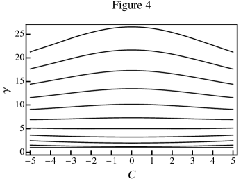
Figure 4: Spatial metric tensor, $\gamma=\gamma_{11}=g_{11}$, for the 1d $c\!\!=\!\!3$ relativistic Gaussian wavepacket of Sec. VI.3, as represented in the natural coordinate frame, $X^{\mu}=(c\,\mathcal{T},C)$. Each curve represents $\gamma$ as a function of $C$ for fixed $\mathcal{T}=\{0,1,2\ldots,10\}$, with increasing $\mathcal{T}$ values corresponding to increasing $\gamma$. At early times, $\mathcal{T}\!>\!0$, the curves bow upward, but at later times they bow downward.

The dynamical behavior of the quantum potential, $Q(\mathcal{T},C)$, is also worthy of discussion. In Fig. 5 are presented curves of $Q$ as a function of $C$, for various fixed values of $\mathcal{T}$ (the same values as in Fig. 4), for the $c\!=\!3$ relativistic Gaussian wavepacket. At $\mathcal{T}\!\!=\!0$, $Q\!\!=\!Q_{0}(C)$ exhibits the usual negative quadratic pattern [Eq. (100)], well known in the context of non-relativistic Gaussian wavepackets. The $Q_{0}(C)$ curve is positive in the interior of the ensemble and negative in the exterior, with the turnover, $Q_{0}(C_{\rm ref})=0$, occurring at $C_{\rm ref}=\pm\sqrt{1/a}=\pm\sqrt{2}$. These points thus serve as the instantaneous demarcation between “classically allowed” and “classically forbidden” regions. A remarkable feature to emerge from Fig. 5 is that these demarcation points are the same for all values of $\mathcal{T}$. In other words, the boundary between allowed and forbidden regions is marked by two special trajectories, $C_{\rm ref}=\pm\sqrt{2}$. We refer to these as “reference trajectories,” because of the fact that $Q\!=\!0$ everywhere along these trajectories, implying from Eq. (75) that $d\tau=d\mathcal{T}$. The proper time, $\tau$, as measured along a reference trajectory, may therefore be used as the dynamical ensemble proper time, $\mathcal{T}$, for the entire trajectory ensemble.

It should be emphasized that the existence of reference trajectories for a given trajectory ensemble is not to be generally expected. We have no general existence proof—nor, indeed, has their existence been mathematically proven even for the relativistic Gaussian wavepacket (although for the $c\!=\!3$ case explicitly considered here, $Q(\mathcal{T},\pm\sqrt{2})=0$ has been established numerically across all $\mathcal{T}$, i.e. not just for the eleven $\mathcal{T}$ values indicated in Fig. 5). That reference trajectories do seem to exist in the relativistic Gaussian case is therefore quite special—perhaps indicating that in some sense, the Gaussian form is preserved, after all. This important property may also provide insight that ultimately makes it possible to arrive at an analytical solution, although to date such efforts have not borne fruit.

Figure 5 also provides—via Eq. (75)—information pertaining to the local time dilation and contraction across the ensemble. We see that these effects are greatest at the initial time, $\mathcal{T}\!\!=\!0$—perhaps counterintuitively, given that the simultaneity submanifold (i.e., the $x$ axis) is least distorted there. Over the course of time, wavepacket broadenening leads to a reduction in the magnitude of $Q(C)$ across all of the trajectories, $C$, and thereby, to a reduction in the time dilation/contraction effect. As discussed, the trajectories in the classically allowed region between the reference trajectories experience time dilation (with the $C\!=\!0$ trajectory experiencing this to the greatest extent), whereas trajectories in the forbidden region experience time contraction.

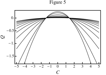
Figure 5: Quantum potential, $Q$, for the 1d $c\!=\!3$ relativistic Gaussian wavepacket of Sec. VI.3, as represented in the natural coordinate frame, $X^{\mu}=(c\,\mathcal{T},C)$. Each curve represents $Q$ as a function of $C$ for fixed $\mathcal{T}=\{0,1,2\ldots,10\}$, with increasing $\mathcal{T}$ values corresponding to flatter curves. $Q\!>\!0$ and $Q\!<\!0$ represent, respectively, the classically allowed and forbidden regions of spacetime. These are demarcated by two special “reference” trajectories, $C_{{\rm ref}}=\pm\sqrt{2}$, along which $Q\!=\!0$ for all time.

VI.4 Hyperbolic wavepacket solutions

In Sec. VI.3, we have seen that the relativistic “Gaussian” wavepacket does not preserve its Gaussian form over time, in the sense that $\rho^{*}(\mathcal{T},C)$ is not Gaussian and $\gamma(\mathcal{T},C)$ depends on $C$, for fixed $\mathcal{T}\!\neq\!0$. This situation begs the question: is there some other choice of $f(C)$, for which the analogous properties do hold? We show in this subsection that such solutions do indeed exist, and moreover, that they can be obtained analytically. It should be stated at the outset, however, that these solutions contain singularities. The solution ensembles also contain trajectories that move along a light cone. Since every simultaneity submanifold includes at least one such trajectory moving at the speed of light, any choice for the initial $\mathcal{T}$ value will lead to initial conditions that necessarily violate the requirements for a viable solution, as laid out in Sec. II. This situation by itself provides sufficient a priori cause to discard these ensembles; hence in that sense, it does not matter that these solutions develop singularities at later or earlier times, because they do not technically belong to our theory. Nevertheless, these solutions are still worth considering because they are simple and analytical, and because they serve as asymptotic limits for other solution ensembles that are in fact viable. For this reason, it will prove instructive to work through them in some detail.

As per the discussion in Sec. VI.3, our starting point will be the condition that $\gamma(\mathcal{T},C)=\gamma(\mathcal{T})$ be independent of $C$. Actually, it will prove beneficial to first consider the special case where

$$\gamma(\mathcal{T})={\rm const}=1\qquad{\rm for}\,\,{\rm all}\,\,\mathcal{T}.$$ (103)

This corresponds to no wavepacket broadening at all, in the sense of the simultaneity submanifolds. However, such solutions—should they prove to exist—will still manifest broadening in $(t,x)$ space, due to the increasing curvature of the simultaneity submanifolds with increasing $\mathcal{T}$ (Sec. VI.3). In any case, the fact that $\gamma\!=\!1$ for all $\mathcal{T}$ and $C$, together with Eq. (V.1), implies that the quantum potential exhibits no $\mathcal{T}$ dependence—i.e., $Q(\mathcal{T},C)=Q_{0}(C)$ for all $\mathcal{T}$. The same must be true for $f^{\mu=1}_{Q}=f^{Q}_{\mu=1}=f_{Q}=-\partial Q/\partial C=-Q_{C}$.

The fact that the force, $f_{Q}(C)$, depends only on $C$ implies that all trajectories in the solution ensemble undergo constant acceleration, in the usual proper time sense. In standard relativity theory, the general form for a trajectory undergoing constant acceleration is well known;rindler ; dolby03 such trajectories trace out hyperbolic orbits. Adopting the initial conditions from the second and third lines of Eq. (100), the solution ensemble must thus be of the following form:

$$t(\tau,C) = {mc\over f_{Q}(C)}\,\sinh\!\left[{{f_{Q}(C)\,\tau\over mc}}\right]$$ (104)

$$x(\tau,C) = {mc\over f_{Q}(C)}\left(\cosh\!\left[{{f_{Q}(C)\,\tau\over mc}}\right]-1\right)+C$$

Next, we convert proper time to ensemble time, using Eq. (75) and the fact that $t=\tau=\mathcal{T}=0$. The result is

$$t(\mathcal{T},C) = {mc\over Q_{C}}\,\sinh\!\left[{{Q_{C}\over mc}\,\exp\!\left({-Q\over mc^{2}}\right)\mathcal{T}}\right],$$ (105)

$$x(\mathcal{T},C) = -{mc\over Q_{C}}\left(\cosh\!\left[{{Q_{C}\over mc}\,\exp\!\left({-Q\over mc^{2}}\right)\mathcal{T}}\right]-1\right)+C.$$

It remains only to find a $Q(C)$ such that Eqs. (13) and (103) are both satisfied. It can be shown that any such $Q(C)$ satisfies

$$f_{Q}(C)^{2}=-mc^{2}f_{Q}^{\prime}(C).$$ (106)

The trivial solution, $f_{Q}(C)=0$, gives rise to the uniform and exponential cases considered in Secs. VI.1 and VI.2, respectively. Otherwise, the most general solution is

$$f_{Q}(C)={mc^{2}\over C},$$ (107)

apart from an immaterial shift in $C$. This leads to

$$Q(C)=-mc^{2}\log[B\,C]\quad;\quad\tau_{\mathcal{T}}(C)=B\,C,$$ (108)

with $B$ an arbitrary constant. Note that $Q(C)$ is singular at the origin.

Finally, substitution of Eqs. (107) and (108) into Eq. (105) leads to remarkably simple explicit forms for the resultant $\gamma\!=\!1$ solutions:

$$t(\mathcal{T},C) = {1\over c}\,C\sinh\!\left[{c\,B\,\mathcal{T}}\right]$$ (109)

$$x(\mathcal{T},C) = C\cosh\!\left[{c\,B\,\mathcal{T}}\right]$$

The simultaneity submanifolds associated with these solutions are straight lines—all intersecting at the origin, which is therefore a singular point. This situation, and Eq. (109) itself, are familiar, in the context of constructing comoving frames for relativistic particles undergoing constant acceleration. As discussed in Sec. I, this leads to multiple reoccurences of the same spacetime events (the origin in this case), and to simultaneous forward ($C>0$) and backward ($C<0$) time propagation.

Of course, it is exactly this type of situation that we sought to avoid with the present formulation. Again, though, we emphasize that the Eq. (109) solution is strictly speaking not a part of our theory, as it can be dismissed based on initial condition considerations alone. More specifically, for the $\mathcal{T}=0$ simultaneity submanifold, the initial conditions are not well-defined at the origin. In effect, there are two trajectories emanating from this point, forming a light cone, and thus moving at the speed of light. In any case, $\mathcal{T}\!\!=\!0$ is ruled out as a viable initial submanifold. At other $\mathcal{T}$ values, the situation is even worse, because Eq. (109) is only defined outside of the light cone—thus leaving gaps where there is no solution at all. As a result, any $\mathcal{T}\neq 0$ also fails to serve as a legitimate initial submanifold, in the sense of Sec. II.

Having obtained a solution to the $\gamma\!=\!1$ problem—albeit a singular one—we next consider the case where $\gamma\!=\!\gamma(\mathcal{T})$. One obvious solution of this type can be easily obtained from Eq. (109), upon realizing that $g_{00}\!=\!g_{00}(C)\!=\!-B^{2}C^{2}$ is independent of $\mathcal{T}$. This is relevant when one considers that simultaneous exchange of $(c\,t,x)$ and $(c\,\mathcal{T},C)$ will flip the roles of $g_{00}$ and $g_{11}$—thus leading to a new dynamical solution undergoing constant (and in fact, zero) acceleration, but for which $g_{11}=\gamma=\gamma(\mathcal{T})$. The analytical form of the new solution is:

$$t(\mathcal{T},C) = \mathcal{T}\!\cosh\!\left[{A\,C}\right]$$ (110)

$$x(\mathcal{T},C) = c\,\mathcal{T}\!\sinh\!\left[{A\,C}\right]$$

Now it is the trajectories of Eq. (110) that are the straight lines intersecting at the origin, with the simultaneity submanifolds the associated hyperbolae. Also, it is now the region inside rather than outside the light cone, that is accessible to the system. In any case, this solution has the same sorts of difficulties as Eq. (109), and can be similarly dismissed. Since the two solutions, Eqs. (109) and (110) explore complementary regions of space, one might consider combining them together. Such an approach would “almost” work, from the perspective of providing reasonable results throughout most of spacetime. However, the origin, and the light cone itself, would still be problematic—thus again making it impossible to find a suitable set of initial conditions for any choice of $\mathcal{T}$.

As we have seen, the solution ensembles developed in this section are not globally viable. Locally, however, they may still serve a useful purpose, particularly as asymptotically limiting forms. For example, a relativistic Gaussian wavepacket in the ultrarelativistic limit of small $c$ or large $a$, is characterized by trajectories that are observed to originate from a small region in space, and to approach their asymptotic straight line forms very quickly. The extreme limit of this behavior would thus correspond to an initially “Dirac delta function” wavepacket, i.e. to Eq. (110).

VII SUMMARY AND CONCLUSIONS

In a series of previous articles, the trajectory-based formulation of non-relativistic quantum mechanics was developed in some detail.bouda03 ; holland05 ; poirier10nowave ; holland10 ; poirier11nowaveCCP6 ; poirier12nowaveJCP ; poirier12ODE What that work offers, in effect, is an alternative—to the usual non-relativistic theory based on the wavefunction, $\Psi$, and the TDSE PDE governing its time evolution. Of course, there are other alternate formulations—and interpretations—of non-relativistic quantum theory,styer02 ; madelung26 ; bohm52a ; bohm52b ; holland ; wyatt ; durr92 ; berndl95 ; einstein35 ; ballentine70 ; home92 ; everett57 ; dewitt70 ; wheeler some of which have been around for a very long time. Almost all of these make use of $\Psi$, or of quantities derived directly from it. The trajectory-based approach stands somewhat apart from these others, because it is formulated independently of $\Psi$ and of the TDSE. Instead, the starting point is the path ensemble ${\bf x}(t,{\bf C})$, from which the solution ensemble is singled out (via the standard Euler-Lagrange prescription) as that which extremizes the non-relativistic quantum action. This leads to the trajectory-based non-relativistic quantum PDE, which happens to be formally equivalent to the TDSE. Thus, even though the resultant quantum trajectories turn out to be identical to those of Bohmian mechanics, the theoretical formulation is completely different—as Bohm’s approach still requires an external $\Psi$ field, to serve as the “pilot wave” governing the quantum trajectory dynamics.

As intriguing as a wavefunction-free formulation of non-relativistic quantum mechanics may be, the fact that the trajectory-based PDE is mathematically equivalent to the TDSE—and to all other non-relativistic quantum formulations, for that matter—suggests that there may be no empirical means available that can distinguish one such theory from another. They may be all equally “correct,” insofar as experiment is concerned. This statement is not meant to diminish the value of the various competing approaches; each has proven to have its own peculiar advantages and disadvantages, vis-à-vis the interpretation, computation, and formulation of the non-relativistic quantum theory.

On the other hand, the approach presented in this document represents a very significant departure from all of these previous efforts. To the author’s best knowledge, the present work represents the only (evidently) viable relativistic quantum formulation for a single spin-zero particle with mass. In this context, the Klein-Gordon (KG) theory is the first and best known competing formalism, although its problems as a single-particle theory are profound (Sec. V.5, and citations therein). More to the present point, however, the KG theory and the present theory make different empirical predictions; they are not mathematically equivalent, and so it should be possible to distinguish between them experimentally. Therefore, regardless of numerical convenience or interpretational elegance, the issue of which theory is “right” is one that can in principle be settled in the laboratory.

No experiment will confirm all of the predictions of KG theory—since these include certain unphysical phenomena such as scattering probabilities that are greater than one.bohm ; holland ; aharonov69 Likewise, the validity of relativity is beyond reproach, and so no experiment performed in the relativistic limit will confirm the predictions of non-relativistic quantum theory—regardless of the particular formulation that is adopted. Such experiments may, however, be able to validate the present relativistic quantum theory, or something similar to it. If this were to happen, then apart from the obvious direct value, it could also shed light on matters of quantum interpretation and ontology that might otherwise linger in the realm of metaphysics rather than science.

This prospect bears some further discussion. Working from the assumption of experimental validation of the sort posited above, one must consider the possibility that there might exist other theoretical formulations, not yet devised, that would lead to formally identical predictions as the present theory—as indeed, we have seen to be the case in the non-relativistic limit. For example, one might well attempt to relativize the other non-relativistic formulations, in analogy with what we have done here for the trajectory-based approach. Such a strategy is likely to fail, however—because the other formulations rely explicitly or implicitly on the TDSE for $\Psi$, whose relativistic generalization is presumably the KG equation. Although the prospect of a viable single-particle relativistic linear wave equation is not entirely ruled out, it seems quite unlikely (Sec. V.5, and discussion below); in any case, no such equation has materialized after more than eighty years. Without such an equation, however, it is not clear how the other, $\Psi$-based non-relativistic formulations are to be relativized, as the linear superposition postulate is not satisfied.bohm ; messiah

Under such hypothetical circumstances, the present formulation—and any associated ontological interpretation—would become the only viable single-particle theory able to explain experimental observation, as opposed to one amongst several equivalent competing theories. As discussed in Sec. II.2, the present approach indeed suggests its own natural “many worlds” interpretation—wherein each trajectory in the ensemble constitutes a distinct world, or universe. This is very different from “conventional” many worlds theory,everett57 ; dewitt70 ; wheeler however. For one thing, the trajectory worlds do interact with each other (which is, indeed, the source of all quantum behavior); for another, the worlds do not branch over time (new trajectories are not “born,” e.g., as a result of measurement, but exist for all time). A further discussion would be out of place in this document, but can be found in our previous work,poirier10nowave ; poirier11nowaveCCP6 ; poirier12nowaveJCP and in future work specifically addressing the quantum measurement ramifications of the trajectory-based approach.

After the above, admittedly speculative discussion, it now behooves us to provide a summary of what has actually been achieved here thus far. The key ideas, in rough order of logical dependence, are listed below:

• General covariance

• Trajectory ensembles

• Simultaneity submanifolds

• Postulate 1: probability conservation along trajectories

• Postulate 2: dynamical forces do not depend on future system states

• Universality of the quantum potential

• Principle of least (or extremal) action

These are the most essential elements, leading to a nearly unambiguous theory of relativistic quantum mechanics, as presented in this work.

Of course, the Einstein Equivalence Principle,carroll ; weinberg or more broadly, the principle of general covariance, pervades everything that we do here—restricting possibilities, and otherwise guiding towards the relativistically proper forms for all quantities. The idea of ensembles of trajectories that foliate spacetime is borrowed from the non-relativistic theory, but is equally natural in the relativistic context, where it is arguably even more important. The reason is that it leads directly to the construction of simultaneity submanifolds for accelerating particles—a central idea of this work, crucial to all of the subsequent development presented here.

A rigorous, global definition of simultaneity is problematic for classical relativistic theory, because a single trajectory can explore only a small portion of spacetime. It is not clear that any such viable notion existed previously—despite certain clever prior developments in this direction, involving intersecting light cones emanating from the worldline, and the like.dolby03 In a trajectory ensemble approach, however, the construction of simultaneity submanifolds is extremely natural and unambiguous. In this respect, the quantum mechanical generalization of relativistic theory actually makes things much easier.

Postulates 1 and 2 provide important insight into the kinematics and dynamics associated with the trajectory ensemble time evolution. One of the most surprising conclusions (at least for the author) to come out of this work is the idea that the KG equation does not satisfy Postulate 2—as reasonable as both the equation and the postulate might seem. The latter is, after all, satisfied by relativistic and non-relativistic classical mechanics, as well as by non-relativistic quantum mechanics; it really should be expected to hold in the relativistic quantum context as well. A quantum application of the Postulate 2 condition logically requires a global notion of simultaneity. Such a structure already exists a priori for the non-relativistic case, but for relativistic applications, seems to require a trajectory ensemble or related approach. In any case, KG theory does not provide a simultaneity structure, leading to an evident causality paradox.

In previous work,poirier11nowaveCCP6 ; poirier12nowaveJCP it has been argued that the quantum potential should adhere to a universal form—which is quite independent of the particular dynamical law (e.g., non-relativistic vs. relativistic). This form can be derived without reference to the TDSE—although the resultant trajectory-based non-relativistic PDE turns out to be equivalent to it, as has been mentioned several times. In the relativistic context, for which there is no previously existing PDE with which to compare, the a priori universality of the $Q$ form obviously plays a central role in the development of the formulation. Finally, of course, the notion of action extremization—so central to classical mechanics, relativity theory and the trajectory-based non-relativistic quantum theory—is also applied to the present relativistic quantum application, placing all of these theories within a single, unified framework.

It is also to be hoped that we may have helped to set the stage for a possible integration with GR, and with quantum gravity. Certainly, our use of general coordinates even in the SR context, lends itself to this purpose—as does the inherent use of density fields. We have, in any case, already uncovered some quite intriguing similarities—and differences—between the gravitational and quantum potentials, as discussed in detail in Sec. V.3. Not least of these is the fact that the value of $Q$ itself—and not just its spatial gradient—plays a dynamical role in its own right, as seen explicitly in the nontrivial example of Sec. VI.3. Also quite relevant (in the non-relativistic context too) is the fact that very narrow wavepackets experience strongly dispersive quantum forces, causing very rapid broadening via trajectory fanout. Thus, on small length scales—i.e., on the order of the Compton wavelength, but still larger than the Planck length—quantum trajectory effects may prevent relativistic singularities from occurring, or may otherwise play an important dynamical role, e.g. in inflation.

There are a number of additional areas for future development that might be considered. Some are straightforward, such as the incorporation of external force fields (e.g., the electromagnetic field for charged particles), and a recasting of the various density and flux quantities into a stress-energy tensor form (together with the development of energy and momentum conservation laws). Less obvious will be determining how to generalize the present theory for multiple particles of fixed number—i.e., the relativistic analog of the many-particle trajectory-based non-relativistic quantum theory already in place. Here, the biggest and most important challenge will be to define simultaneity submanifolds for multiple particles. This is not so straightforward, and may well prove to be the “Achilles’ heel” of the present approach—most likely related to the oft-quoted claim that relativistic theories involving interaction energies comparable to particle rest masses must encompass the creation/annihilation of particles.bohm ; messiah Of course, one might also attempt to apply some of the current ideas in a varying-particle-number, QFT context. Given the difficulties of the KG equation, one wonders whether it is correct to use this as a basis for QFT, as is currently accepted practice. How would things change if the present approach were adopted instead? What impact might this have, e.g., on theoretical predictions pertaining to the Higgs boson or pi meson?

Of course, the basic ideas developed here need not be limited to massive spin-zero bosons. It is only natural that one might consider revisiting the Dirac field for spin 1/2 particles, as well as the quantized electromagnetic field describing photons, armed with the weapons developed in the present arsenal. It is not yet clear what such investigations might turn up—i.e., whether they would lead to new theoretical predictions, as they seem to have done in the present case for spin-zero particles, or to predictions in substantive agreement with currently accepted theories. In the photon context, of course, the simultaneity submanifold concept per se would have to be discarded—presumably, to be replaced with an analogous family of null hypersurfaces. It is not yet clear whether this would even be possible.

Even for the specific relativistic quantum PDEs developed here, there is still much work that remains to be done, in terms of characterizing these fully. Can an analytical solution for the relativistic Gaussian (or other nontrival) wavepacket be derived? Are the solution ensembles always well-behaved (subject to the conditions of Sec. II), or is it possible that singularities can somehow develop? Are the PDEs inherently nonlinear, or can they be recast into an equivalent linear wave equation? Under what conditions is numerical solution of the PDEs unstable, and what sorts of algorithms can be used or should be developed?

One very basic property of particular interest has already been established. This is simply that the PDE order in the spatial coordinates $({\bf C})$ is twice that in the time coordinate ($\mathcal{T}$)—even though these equations are perfectly invariant with respect to Lorentz transformations. This is not surprising in one sense—i.e., in light of the theoretical developments presented in this document (notably pertaining to Postulate 2). In the context of the history of relativistic wave equations, on the other hand, it is highly unusual—if not borderline heretical. Traditional treatments virtually always presume that the space and time orders must be identical, in order to treat these coordinates on an equal footing. The present theory, in contrast, suggests that there is indeed a fundamental difference between space and time—at least when these notions are interpreted in an appropriate manner, and linked to a single particle/observer.

In any case, it should be mentioned that the two-to-one ratio of space-to-time orders that characterizes the present relativistic quantum PDEs as described above, also characterizes the non-relativistic quantum PDEs—both the trajectory-based PDE, and the TDSE itself. This is, in large measure, why the present theory reduces so seamlessly to these others in the non-relativistic limit. One might also do well to recall that it is precisely the lack of such an asymmetry in the KG equation—i.e., the fact that this equation is second-order in both space and time—that is known to lead to the difficulties described in Sec. V.5, especially that of defining a suitable probability density quantity. These problems were well understood in the early days of the quantum theory—but what is perhaps quite startling is that the same can be said of all of the theoretical tools used here to develop the present fix (though of course, the trajectory-based formulation itself is new). In principle, Einstein or Dirac, or one of their contemporaries, could have hit upon this very same approach. One (at least the author) has to wonder how things might have progressed differently, had this idea been born in say, 1932, or even 1952,bohm52a ; bohm52b rather than in 2012.

References

- (1) J. von Neumann, in Mathematical Foundations of Quantum Mechanics (Princeton University Press, New Jersey, 1932).
- (2) C. Cohen-Tannoudji, Quantum Mechanics (Wiley, New York, 1977).
- (3) D. Bohm, Quantum Theory (Dover, New York, 1979).
- (4) D. M. McQuarrie, Quantum Chemistry (University Science Books, Mill Valley, CA, 1983).
- (5) A. Messiah, Quantum Mechanics (Dover, New York, 1999).
- (6) D. Styer, Am. J. Phys. 70, 288 (2002).
- (7) E. Madelung, Z. Phys. 40, 322 (1926).
- (8) D. Bohm, Phys. Rev. 85, 166 (1952).
- (9) D. Bohm, Phys. Rev. 85, 180 (1952).
- (10) P. R. Holland, The Quantum Theory of Motion (Cambridge University Press, Cambridge, 1993).
- (11) R. E. Wyatt, Quantum Dynamics with Trajectories: Introduction to Quantum Hydrodynamics (Springer, New York, 2005).
- (12) D. Dürr, S. Goldstein, and N. Zanghì, J. Stat. Phys. 67, 843 (1992).
- (13) K. Berndl, M. Daumer, D. Dürr, S. Golstein, and N. Zanghì, Il Nuovo Cimento 110B, 737 (1995).
- (14) A. Einstein, B. Podolsky, and N. Rosen, Phys. Rev. 47, 777 (1935).
- (15) L. E. Ballentine, Rev. Mod. Phys. 42, 358 (1970).
- (16) D. Home and M. A. B. Whittaker, Phys. Rep. 210, 223 (1992).
- (17) H. Everett III, Rev. Mod. Phys. 29, 454 (1957).
- (18) B. S. Dewitt, Physics Today 23, 30 (1970).
- (19) Quantum Theory of Measurement, edited by J. A. Wheeler and W. H. Zurek (Princeton University Press, Princeton, 1983).
- (20) A. Bouda, Int. J. Mod. Phys. A 18, 3347 (2003).
- (21) P. Holland, Ann. Phys. 315, 505 (2005).
- (22) B. Poirier, Chem. Phys. 370, 4 (2010).
- (23) P. Holland, in Quantum Trajectories, edited by P. Chattaraj (Taylor and Francis/CRC Press, Boca Raton, 2010), Chap. 5, pp. 73–85.
- (24) B. Poirier, in Quantum Trajectories, edited by K. H. Hughes and G. Parlant (CCP6, Daresbury Laboratory, 2011), Chap. Trajectory-Based Derivation of Classical and Quantum Mechanics, p. 6.
- (25) J. Schiff and B. Poirier, J. Chem. Phys. 136, 031102 (2012).
- (26) G. Parlant, Y.-C. Ou, K. Park, and B. Poirier, Comput. Theoret. Chem. 990, 3 (2012).
- (27) http://press.web.cern.ch/press/PressReleases/Releases 2012/PR17.12E.html.
- (28) I. Bialynicki-Birula, Acta Phys. Polonica A 86, 97 (1994).
- (29) J. E. Sipe, Phys. Rev. A 52, 1875 (1995).
- (30) P. Rosenau and Z. Schuss, Phys. Lett. A 375, 891 (2011).
- (31) L. de Broglie, Nonlinear Wave Mechanics (Gauthier-Villars, Paris, 1956).
- (32) H. Feshbach and F. Villars, Rev. Mod. Phys. 30, 24 (1958).
- (33) S. M. Carroll, An Introduction to General Relativity Spacetime and Geometry (Addison-Wesley, San Francisco, 2004).
- (34) Y. Aharonov, A. Komar, and L. Susskind, Phys. Rev. 182, 1400 (1969).
- (35) D. I. Blokhintsev, Space and Time in the Microworld (D. Reidel, Dordrecht, 1973).
- (36) A. F. Rañada and G. S. Rodero, Phys. Rev. D 22, 385 (1980).
- (37) A. Kyprianidis, Phys. Lett. 111, 111 (1985).
- (38) P. A. M. Dirac, Proc. Roy. Soc. London A 117, 610 (1928).
- (39) P. A. M. Dirac, Proc. Roy. Soc. London A 118, 351 (1928).
- (40) W. E. Thirring, Principles of Quantum Electrodynamics (Academic Press, New York, 1958).
- (41) N. N. Bogoliubov and D. V. Shirkov, Introduction to the Theory of Quantized Fields (Interscience Publishers, Inc., New York, 1959).
- (42) S. S. Schweber, An Introduction to Relativistic Quantum Field Theory (Row, Peterson and Company, New York, 1961).
- (43) S. Weinberg, Gravitation and Cosmology (Wiley, New York, 1972).
- (44) W. Rindler, Relativity (Oxford University Press, UK, 2006).
- (45) C. E. Dolby, arXiv:gr-qc/0305097 (2003).
- (46) B. Schutz, Geometrical Methods of Mathematical Physics (Cambridge University Press, Cambridge, UK, 1980).