The distribution function of the distance between two random points in a right-angled triangle

Abstract

In this paper we obtain the density function and the distribution function of the distance between two uniformly and independently distributed random points in any right-angled triangle. The density function is derived from the chord length distribution function using Piefke’s formula. We conclude results for random distances between two congruent right-angled triangles together forming a rectangle.
2010 Mathematics Subject Classification: 60D05, 52A22
Keywords: Geometric probability, random sets, integral geometry, chord length distribution function, random distances, distance distribution function, right-angled triangles, right triangle, Piefke formula

1 Introduction

A random line $g$ intersecting a convex set $\mathcal{K}$ in the plane produces a chord of $\mathcal{K}$. The length $s$ of this chord is a random variable. The chord length distribution function of a regular triangle was calculated by Sulanke [14, p. 57]. Harutyunyan and Ohanyan [8] calculated the chord length distribution function for regular polygons (see also Bäsel [2, pp. 2-9]).

The distance $t$ between two points chosen independently and uniformly at random from $\mathcal{K}$ is also a random variable. Borel [3] considered random distances in elementary geometric figures such as triangles, squares and so on (see [11, p. 163]). The expectations of the distance between two random points for an equilateral triangle and a rectangle are to be found in [13, p. 49]. Ghosh [6] derived the distance density function for a rectangle. Bäsel [2, pp. 10-16] derived the density function and the distribution function of the distance for regular polygons from its chord length distribution function using Piefke’s formula [12, p. 130]. There are a lot of results concerning the distance $t$ within a convex set or in two convex sets, see Chapter 2 in [10].

For practical applications in physics, material sciences, operations research, communication networks and other fields see [7], [9] and [15].

The first aim of the present paper is to derive the chord length distribution function for any right-angled triangle. The second aim is to conclude the distribution function of the distance between two points chosen independently and uniformly from a right-angled triangle.

$A=(0,b)$, $B=(a,0)$ and $C=(0,0)$ are the vertices of the right-angled triangle (see Fig. 1b). We assume $|\overline{AC}|=b\geq a=|\overline{BC}|$ and denote this triangle by $\mathcal{T}_{a,\;\!b}$. Clearly, it is possible to bring every right-angled triangle in such a position by use of Euclidean motions (translations and rotations) and, if necessary, a reflection. These operations do not influence the chord length distribution and the point distance distribution. $c=|\overline{AB}|$ is the length of the hypotenuse and $\alpha=\arctan(a/b)$ the inner angle between $\overline{AB}$ and $\overline{AC}$. $u=a+b+c$ is the length of the perimeter of $\mathcal{T}_{a,\;\!b}$, $\tilde{A}=ab/2$ its area and $h=a\cos\alpha$ the height over $\overline{AB}$. The hypotenuse $\overline{AB}$ of the triangle $\mathcal{T}_{a,\;\!b}$ is the diameter of its circumcircle (converse of Thales’ theorem).

2 Chord length distribution function

A straight line $g$ in the plane is determined by the angle $\psi$, $0\leq\psi<2\pi$, that the direction perpendicular to $g$ makes with a fixed direction (e.g. the $x$-axis) and by its distance $p$, $0\leq p<\infty$, from the origin $O$:

$$g=g(p,\psi)=\{(x,y)\in\mathbb{R}^{2}:\,x\cos\psi+y\sin\psi=p\}\,.$$

The measure $\mu$ of a set of lines $g(p,\psi)$ is defined by the integral, over the set, of the differential form $\mathrm{d}g=\mathrm{d}p\>\mathrm{d}\psi$. Up to a constant factor, this measure is the only one that is invariant under motions in the Euclidean plane [13, p. 28].

We use the chord length distribution function of $\mathcal{T}_{a,\;\!b}$ in the form

$$F(s)=\frac{1}{u}\>\mu(\{g:\,g\cap\mathcal{T}_{a,\;\!b}\not=\emptyset,\,|\chi(g)|\leq s\})\,,$$

where $\chi(g)=g\cap\mathcal{T}_{a,\;\!b}$ is the chord of $\mathcal{T}_{a,\;\!b}$, produced by the line $g$, and $|\chi(g)|$ the length of $\chi(g)$ (see [5, p. 863] and [1, p. 161]). (The measure of all lines $g$ that intersect a convex set is equal to its perimeter [13, p. 30].) So it remains to calculate the measure of all lines that produce a chord of length $|\chi(g)|\leq s$ . Using the abbreviation

$$\mathcal{S}(g,\>\!s):=\{g:\,g\cap\mathcal{T}_{a,\;\!b}\not=\emptyset,\,|\chi(g)|\leq s\}\,,$$

we have

$$\mu(\mathcal{S}(g,\>\!s))=\int_{\mathcal{S}(g,\>\!s)}\,\mathrm{d}g=\int_{\mathcal{S}(g,\>\!s)}\,\mathrm{d}p\>\mathrm{d}\psi\,.$$

Instead of the angle $\psi$ it is possible to use the angle $\phi$ that a line makes with the positive $x$-axis, hence

$$\mu(\mathcal{S}(g,\>\!s))=\int_{\mathcal{S}(g,\>\!s)}\,\mathrm{d}p\>\mathrm{d}\phi\,.$$

Theorem 1.

The chord length distribution function $F$ of $\mathcal{T}_{a,\;\!b}$ is given by

$$F(s)=\left\{\begin{array}[]{lcl}0&\mbox{if}&s<0\,,\\[2.84544pt] H_{1}(s)/u&\mbox{if}&0\leq s<h\,,\\[2.84544pt] H_{2}(s)/u&\mbox{if}&h\leq s<a\,,\\[2.84544pt] H_{3}(s)/u&\mbox{if}&a\leq s<b\,,\\[2.84544pt] H_{4}(s)/u&\mbox{if}&b\leq s<c\,,\\[2.84544pt] 1&\mbox{if}&s\geq c\,,\end{array}\right.$$

where

$$H_{1}(s)={} \frac{\Theta_{1}\,s}{4}\,,$$

$$H_{2}(s)={} \frac{\Theta_{2}\,s}{4}+\Theta_{3}\,L_{1}(s,h)+c\,L_{2}(s,h)\,,$$

$$H_{3}(s)={} a+\Theta_{4}\,s+\frac{\Theta_{3}}{2}\,L_{1}(s,h)+\frac{c}{2}\,L_{2}(s,h)+\frac{b}{2a}\,L_{1}(s,a)+\frac{b}{2}\,L_{2}(s,a)\,,$$

$$H_{4}(s)={} \Theta_{5}+\frac{\Theta_{6}\,s}{4}+\frac{b}{2a}\,L_{1}(s,a)+\frac{b}{2}\,L_{2}(s,a)+\frac{a}{2b}\,L_{1}(s,b)+\frac{a}{2}\,L_{2}(s,b)$$

with

$$\Theta_{1}={} \frac{a}{b}\,(2\alpha+\pi)+\frac{2b}{a}\,(\pi-\alpha)+6\;,\;\;\Theta_{2}=\frac{a}{b}\,(2\alpha-\pi)-\frac{2b}{a}\,\alpha+6\,,$$

$$\Theta_{3}={} \frac{a}{b}+\frac{b}{a}\;,\;\;\Theta_{4}=1-\frac{b}{a}\,\alpha\;,\;\;\Theta_{5}=a+b\;,\;\;\Theta_{6}=\frac{a}{b}\,(2\alpha-\pi)-\frac{2b}{a}\,\alpha+2$$

and

$$L_{1}(s,a)=s\arcsin\frac{a}{s}\;,\quad L_{2}(s,a)=\sqrt{1-\left(\frac{a}{s}\right)^{2}}\;.$$

Proof.

In the following we need the width $w$ of $\mathcal{T}_{a,\;\!b}$ in the direction perpendicular to the angle $\phi$ that is given by:

$$w(\phi)=\left\{\begin{array}[]{lcl}w_{1}(\phi)&\mbox{if}&0\leq\phi<\pi/2\,,\\[2.84544pt] w_{2}(\phi)&\mbox{if}&\pi/2\leq\phi<\pi/2+\alpha\,,\\[2.84544pt] w_{3}(\phi)&\mbox{if}&\pi/2+\alpha\leq\phi\leq\pi\,,\end{array}\right.$$

where

$$w_{1}(\phi)=a\,\frac{\cos(\phi-\alpha)}{\sin\alpha}\;,\quad w_{2}(\phi)=a\sin\phi\;,\quad w_{3}(\phi)=-a\,\frac{\cos\phi}{\tan\alpha}\;.$$

We have to distinguish the cases $0\leq s<h$, $h\leq s<a$, $a\leq s<b$ and $b\leq s<c$, and put

$$\begin{array}[]{llc@{\;,\quad}llc}H_{1}(s)=\mu(\mathcal{S}(g,\>\!s))&\mbox{if}&0\leq s<h&H_{2}(s)=\mu(\mathcal{S}(g,\>\!s))&\mbox{if}&h\leq s<a\;,\\[2.84544pt] H_{3}(s)=\mu(\mathcal{S}(g,\>\!s))&\mbox{if}&a\leq s<b&H_{4}(s)=\mu(\mathcal{S}(g,\>\!s))&\mbox{if}&b\leq s<c\;.\end{array}$$

We demonstrate the calculation of $H_{2}$. Here it is necessary to distinguish the following intervals of $\phi$ (see Fig. 1) :

• $0\leq\phi<\phi_{1}=\alpha-\arccos\left((a/s)\cos\alpha\right)$ : All lines $g$ with fixed angle $\phi$ produce a chord $\chi$ of length $|\chi(g)|\leq s$ if they are lying in one of the two strips of breadth

  $$b_{1}(s,\phi)=\frac{s}{2}\,\frac{\sin(2\phi-\alpha)+\sin\alpha}{\cos\alpha}\;\;\mbox{and}\;\;b_{2}(s,\phi)=\frac{s}{2}\,\frac{\cos(2\phi-\alpha)+\cos\alpha}{\sin\alpha}$$

  respectively.

• $\phi_{1}\leq\phi<\phi_{2}=\alpha+\arccos\left((a/s)\cos\alpha\right)$ : All lines $g$ with fixed angle $\phi$ and $g\cap\mathcal{T}_{a,\;\!b}\not=\emptyset$ produce a chord of length $|\chi(g)|\leq s$. These lines are lying in a strip of breadth $w_{1}(\phi)$.

• $\phi_{2}\leq\phi<\pi/2$ : See $0\leq\phi<\phi_{1}$.

• $\pi/2\leq\phi<\pi/2+\alpha$ : All lines $g$ with fixed angle $\phi$ produce a chord of $\mbox{length}\leq s$ if they are lying in one of the two strips of breadth $b_{1}(s,\phi)$ and

  $$b_{3}(s,\phi)=-\frac{s}{2}\,\sin 2\phi$$

  respectively.

• $\pi/2+\alpha\leq\phi<\pi$ : All lines $g$ with fixed angle $\phi$, lying in one of the two strips of breadth $b_{2}(s,\phi)$ and $b_{3}(s,\phi)$ repectively, produce a chord of length $\leq s$.

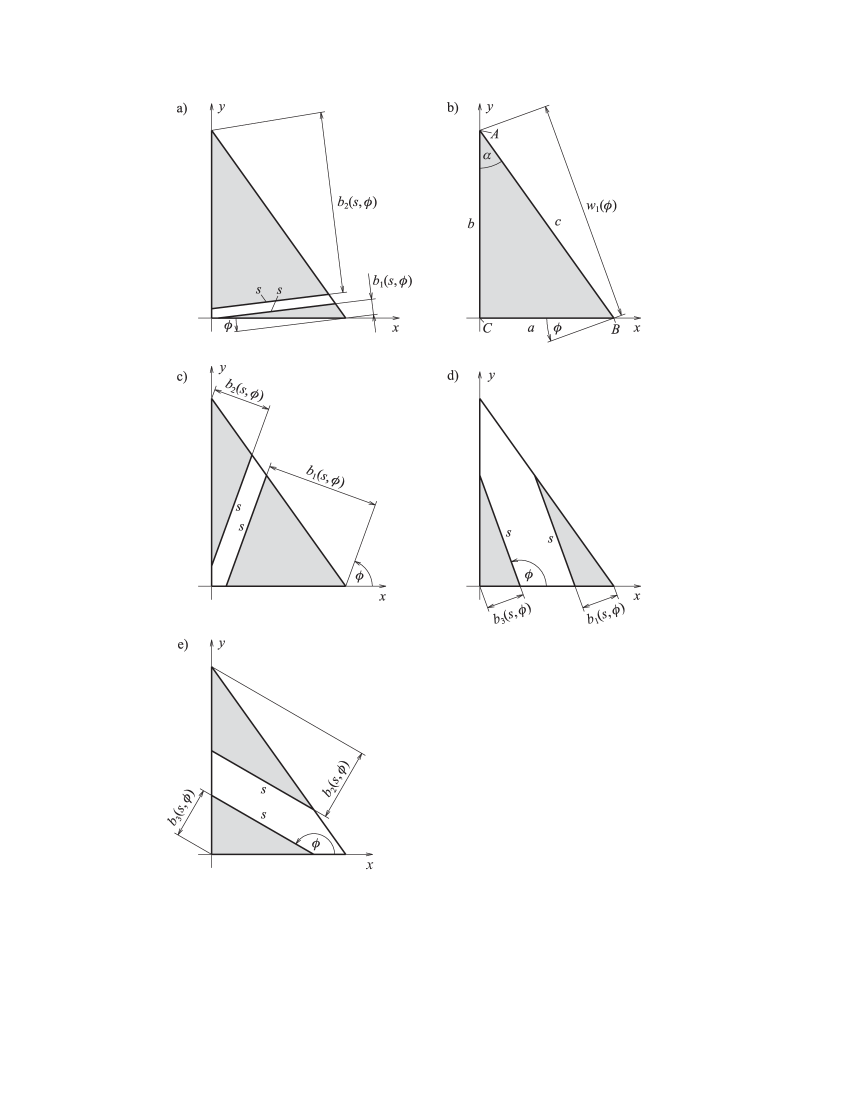
Figure 1: Calculation of $H_{2}$

Therefore, using the abbreviations $b_{i}$ and $w_{i}$ for $b_{i}(s,\phi)$ and $w_{i}(\phi)$ respectively,

$$H_{2}(s)=\int_{\mathcal{S}(g,\>\!s)}\,\mathrm{d}p\>\mathrm{d}\phi={} \int_{0}^{\phi_{1}}(b_{1}+b_{2})\,\mathrm{d}\phi+\int_{\phi_{1}}^{\phi_{2}}w_{1}\,\mathrm{d}\phi+\int_{\phi_{2}}^{\pi/2}(b_{1}+b_{2})\,\mathrm{d}\phi$$

$$+\int_{\pi/2}^{\pi/2+\alpha}(b_{1}+b_{3})\,\mathrm{d}\phi+\int_{\pi/2+\alpha}^{\pi}(b_{2}+b_{3})\,\mathrm{d}\phi\,.$$

With the angles

$$\phi_{3}=\pi-\arccos\dfrac{a}{s}\quad\mbox{and}\quad\phi_{4}=\pi-\arcsin\left(\dfrac{a}{s}\,\cot\alpha\right)$$

we analogously get

$$H_{1}(s)={} \int_{0}^{\pi/2}(b_{1}+b_{2})\,\mathrm{d}\phi+\int_{\pi/2}^{\pi/2+\alpha}(b_{1}+b_{3})\,\mathrm{d}\phi+\int_{\pi/2+\alpha}^{\pi}(b_{2}+b_{3})\,\mathrm{d}\phi\,,$$

$$H_{3}(s)={} \int_{0}^{\phi_{2}}w_{1}\,\mathrm{d}\phi+\int_{\phi_{2}}^{\pi/2}(b_{1}+b_{2})\,\mathrm{d}\phi+\int_{\pi/2}^{\pi/2+\alpha}(b_{1}+b_{3})\,\mathrm{d}\phi$$

$$+\int_{\pi/2+\alpha}^{\phi_{3}}(b_{2}+b_{3})\,\mathrm{d}\phi+\int_{\phi_{3}}^{\pi}w_{3}\,\mathrm{d}\phi\,,$$

$$H_{4}(s)={} \int_{0}^{\pi/2}w_{1}\,\mathrm{d}\phi+\int_{\pi/2}^{\phi_{4}}w_{2}\,\mathrm{d}\phi+\int_{\phi_{4}}^{\pi/2+\alpha}(b_{1}+b_{3})\,\mathrm{d}\phi$$

$$+\int_{\pi/2+\alpha}^{\phi_{3}}(b_{2}+b_{3})\,\mathrm{d}\phi+\int_{\phi_{3}}^{\pi}w_{3}\,\mathrm{d}\phi\,.$$

Using the indefinite integrals

$$\int b_{1}(s,\phi)\,\mathrm{d}\phi={} \frac{s}{4}\,\frac{2\phi\sin\alpha-\cos(2\phi-\alpha)}{\cos\alpha}\,,$$

$$\int b_{2}(s,\phi)\,\mathrm{d}\phi={} \frac{s}{4}\,\frac{2\phi\cos\alpha+\sin(2\phi-\alpha)}{\sin\alpha}\,,$$

$$\int b_{3}(s,\phi)\,\mathrm{d}\phi={} \frac{s}{2}\,\cos^{2}\phi\,,$$

$$\int w_{1}(\phi)\,\mathrm{d}\phi\>\,={} \frac{a\sin(\phi-\alpha)}{\sin\alpha}=a(\cot\alpha\sin\phi-\cos\phi)\,,$$

$$\int w_{2}(\phi)\,\mathrm{d}\phi\>\,={} -a\cos\phi\;,\quad\int w_{3}(\phi)\,\mathrm{d}\phi=-\frac{a\sin\phi}{\tan\alpha}\,,$$

one finds the result of Theorem 1. ∎

Remark.

It is easy to derive the chord length density function from Theorem 1.

3 Point distances

Theorem 2.

The density function $g$ of the distance $t$ between two random points in $\mathcal{T}_{a,\;\!b}$ is given by

$$g(t)=\left\{\begin{array}[]{ll}\dfrac{2t}{\tilde{A}}\left[\pi+\dfrac{1}{\tilde{A}}\,(J^{*}(t)-ut)\right]&\mbox{if}\quad 0\leq t\leq c\,,\\[11.38092pt] 0&\mbox{else}\,,\end{array}\right.$$

where

$$J^{*}(t)=\left\{\begin{array}[]{lcl}J_{1}^{*}(0,t)&\mbox{if}&0\leq t<h\,,\\[2.84544pt] J_{1}^{*}(0,h)+J_{2}^{*}(h,t)&\mbox{if}&h\leq t<a\,,\\[2.84544pt] J_{1}^{*}(0,h)+J_{2}^{*}(h,a)+J_{3}^{*}(a,t)&\mbox{if}&a\leq t<b\,,\\[2.84544pt] J_{1}^{*}(0,h)+J_{2}^{*}(h,a)+J_{3}^{*}(a,b)+J_{4}^{*}(b,t)&\mbox{if}&b\leq t\leq c\end{array}\right.$$

with

$$J_{k}^{*}(s,t)=H_{k}^{*}(t)-H_{k}^{*}(s)\,,$$

where

$$H_{1}^{*}(t)={} \frac{\Theta_{1}\,t^{2}}{8}\,,$$

$$H_{2}^{*}(t)={} \frac{\Theta_{2}\,t^{2}}{8}+\Theta_{3}\,L_{1}^{*}(t,h)+c\,L_{2}^{*}(t,h)\,,$$

$$H_{3}^{*}(t)={} at+\frac{\Theta_{4}\,t^{2}}{2}+\frac{\Theta_{3}}{2}\,L_{1}^{*}(t,h)+\frac{c}{2}\,L_{2}^{*}(t,h)+\frac{b}{2a}\,L_{1}^{*}(t,a)+\frac{b}{2}\,L_{2}^{*}(t,a)\,,$$

$$H_{4}^{*}(t)={} \Theta_{5}\,t+\frac{\Theta_{6}\,t^{2}}{8}+\frac{b}{2a}\,L_{1}^{*}(t,a)+\frac{b}{2}\,L_{2}^{*}(t,a)+\frac{a}{2b}\,L_{1}^{*}(t,b)+\frac{a}{2}\,L_{2}^{*}(t,b)$$

with

$$L_{1}^{*}(t,a)={} \frac{1}{2}\left(a\sqrt{t^{2}-a^{2}}+t^{2}\arcsin\frac{a}{t}\right)\,,\;\;L_{2}^{*}(t,a)=\sqrt{t^{2}-a^{2}}+a\arcsin\frac{a}{t}\,.$$

Proof.

According to a theorem of Piefke [12, p. 130], the density function of the distance between two random points is given by

$$g(t)=\frac{2ut}{\tilde{A}^{2}}\int_{t}^{c}(s-t)f(s)\,\mathrm{d}s\,,$$

where $f$ is the density function of the chord length. Following [2, pp. 11/12], we obtain

$$g(t)=\frac{2t}{\tilde{A}}\left[\pi-\frac{u}{\tilde{A}}\left(t-\int_{0}^{t}F(s)\,\mathrm{d}s\right)\right]=\frac{2t}{\tilde{A}}\left[\pi+\frac{1}{\tilde{A}}\,(J^{*}(t)-ut)\right]$$

with

$$J^{*}(t):=u\int_{0}^{t}F(s)\,\mathrm{d}s\,.$$

This yields for $0\leq t<h$

$$J^{*}(t)=\int_{0}^{t}H_{1}(s)\,\mathrm{d}s=H_{1}^{*}(t)-H_{1}^{*}(0)=J_{1}^{*}(0,t)\,,$$

and for $h\leq t<a$

$$J^{*}(t)={} u\int_{0}^{t}F(s)\,\mathrm{d}s=\int_{0}^{h}H_{1}(s)\,\mathrm{d}s+\int_{h}^{t}H_{2}(s)\,\mathrm{d}s$$

$$={} H_{1}^{*}(h)-H_{1}^{*}(0)+H_{2}^{*}(t)-H_{2}^{*}(h)=J_{1}^{*}(0,h)+J_{2}^{*}(h,t)\,.$$

The calculations of $J^{*}(t)$ for the intervals $a\leq t<b$ and $b\leq t<c$ can be carried out in the same manner.

Now we determine the indefinite integrals of $L_{1}(t,a)$ and $L_{2}(t,a)$. Using integration by parts, we find

$$L_{1}^{*}(t,a)={} \int L_{1}(t,a)\,\mathrm{d}t=\int t\arcsin\frac{a}{t}\;\mathrm{d}t$$

$$={} \frac{1}{2}\left(t^{2}\arcsin\frac{a}{t}+a\int\frac{t}{\sqrt{t^{2}-a^{2}}}\;\mathrm{d}t\right).$$

Clearly,

$$\int\frac{t}{\sqrt{t^{2}-a^{2}}}\;\mathrm{d}t=\sqrt{t^{2}-a^{2}}$$

and therefore

$$L_{1}^{*}(t,a)=\frac{1}{2}\left(a\sqrt{t^{2}-a^{2}}+t^{2}\arcsin\frac{a}{t}\right).$$

Since $t\geq a>0$ in the present cases,

$$L_{2}^{*}(t,a)={} \int L_{2}(t,a)\,\mathrm{d}t=\int\sqrt{1-\left(\frac{a}{t}\right)^{2}}\;\mathrm{d}t=\int\frac{\sqrt{t^{2}-a^{2}}}{t}\;\mathrm{d}t\,,$$

and (cf. [4, p. 48, Eq. 217])

$$L_{2}^{*}(t,a)=\sqrt{t^{2}-a^{2}}+a\arcsin\frac{a}{t}\,.\qed$$

Corollary 1.

The distribution function $G$ of the distance $t$ between two random points in $\mathcal{T}_{a,\;\!b}$ is given by

$$G(t)=\left\{\begin{array}[]{lcl}0&\mbox{if}&t<0\,,\\[5.69046pt] \dfrac{1}{\tilde{A}}\left[t^{2}\left(\pi-\dfrac{2u}{3\tilde{A}}\,t\right)+\dfrac{2}{\tilde{A}}\,J^{\natural}(t)\right]&\mbox{if}&0\leq t<c\,,\\[11.38092pt] 1&\mbox{if}&t\geq c\end{array}\right.$$

with

$$J^{\natural}(t)=\left\{\begin{array}[]{lcl}K_{1}(t)&\mbox{if}&0\leq t<h\,,\\[2.84544pt] K_{1}(h)+K_{2}(t)&\mbox{if}&h\leq t<a\,,\\[2.84544pt] K_{1}(h)+K_{2}(a)+K_{3}(t)&\mbox{if}&a\leq t<b\,,\\[2.84544pt] K_{1}(h)+K_{2}(a)+K_{3}(b)+K_{4}(t)&\mbox{if}&b\leq t<c\,,\end{array}\right.$$

where

$$K_{1}(t)={} J_{1}^{\natural}(0,t)\,,$$

$$K_{2}(t)={} \frac{1}{2}\left(t^{2}-h^{2}\right)[J_{1}^{*}(0,h)-H_{2}^{*}(h)]+J_{2}^{\natural}(h,t)\,,$$

$$K_{3}(t)={} \frac{1}{2}\left(t^{2}-a^{2}\right)[J_{1}^{*}(0,h)+J_{2}^{*}(h,a)-H_{3}^{*}(a)]+J_{3}^{\natural}(a,t)\,,$$

$$K_{4}(t)={} \frac{1}{2}\left(t^{2}-b^{2}\right)[J_{1}^{*}(0,h)+J_{2}^{*}(h,a)+J_{3}^{*}(a,b)-H_{4}^{*}(b)]+J_{4}^{\natural}(b,t)$$

with $J_{k}^{*}$ and $H_{k}^{*}$ according to Theorem 2 and

$$J_{k}^{\natural}(s,t)=H_{k}^{\natural}(t)-H_{k}^{\natural}(s)\,,$$

where

$$H_{1}^{\natural}(t)={} \frac{\Theta_{1}\,t^{4}}{32}\,,$$

$$H_{2}^{\natural}(t)={} \frac{\Theta_{2}\,t^{4}}{32}+\Theta_{3}\,L_{1}^{\natural}(t,h)+c\,L_{2}^{\natural}(t,h)\,,$$

$$H_{3}^{\natural}(t)={} \frac{at^{3}}{3}+\frac{\Theta_{4}\,t^{4}}{8}+\frac{\Theta_{3}}{2}\,L_{1}^{\natural}(t,h)+\frac{c}{2}\,L_{2}^{\natural}(t,h)+\frac{b}{2a}\,L_{1}^{\natural}(t,a)+\frac{b}{2}\,L_{2}^{\natural}(t,a)\,,$$

$$H_{4}^{\natural}(t)={} \frac{\Theta_{5}\,t^{3}}{3}+\frac{\Theta_{6}\,t^{4}}{32}+\frac{b}{2a}\,L_{1}^{\natural}(t,a)+\frac{b}{2}\,L_{2}^{\natural}(t,a)+\frac{a}{2b}\,L_{1}^{\natural}(t,b)+\frac{a}{2}\,L_{2}^{\natural}(t,b)$$

with

$$L_{1}^{\natural}(t,a)={} \frac{1}{8}\left[\frac{5a}{3}\left(t^{2}-a^{2}\right)^{3/2}+a^{3}\,\sqrt{t^{2}-a^{2}}+t^{4}\arcsin\frac{a}{t}\right]\,,$$

$$L_{2}^{\natural}(t,a)={} \frac{1}{3}\left(t^{2}-a^{2}\right)^{3/2}+\frac{a}{2}\left(a\sqrt{t^{2}-a^{2}}+t^{2}\,\arcsin\frac{a}{t}\right)\,.$$

Proof.

For $0\leq t<c$ one gets

$$G(t)={} \int_{0}^{t}g(\tau)\,\mathrm{d}\tau=\int_{0}^{t}\left(\frac{2\pi\tau}{\tilde{A}}-\frac{2u\tau^{2}}{\tilde{A}^{2}}+\frac{2u\tau}{\tilde{A}^{2}}\int_{0}^{\tau}F(s)\,\mathrm{d}s\right)\mathrm{d}\tau$$

$$={} \frac{\pi t^{2}}{\tilde{A}}-\frac{2ut^{3}}{3\tilde{A}^{2}}+\frac{2u}{\tilde{A}^{2}}\int_{0}^{t}\tau\left(\int_{0}^{\tau}F(s)\,\mathrm{d}s\right)\mathrm{d}\tau$$

$$={} \frac{\pi t^{2}}{\tilde{A}}-\frac{2ut^{3}}{3\tilde{A}^{2}}+\frac{2}{\tilde{A}^{2}}\int_{0}^{t}\tau J^{*}(\tau)\,\mathrm{d}\tau=\frac{1}{\tilde{A}}\left[t^{2}\left(\pi-\dfrac{2u}{3\tilde{A}}\,t\right)+\dfrac{2}{\tilde{A}}\,J^{\natural}(t)\right]$$

with

$$J^{\natural}(t):=\int_{0}^{t}sJ^{*}(s)\,\mathrm{d}s\,.$$

It remains to calculate $J^{\natural}(t)$. For $0\leq t<h$ we have

$$J^{\natural}(t)={} \int_{0}^{t}sJ_{1}^{*}(0,s)\,\mathrm{d}s=\int_{0}^{t}s\,[H_{1}^{*}(s)-H_{1}^{*}(0)]\,\mathrm{d}s$$

$$={} H_{1}^{\natural}(t)-H_{1}^{\natural}(0)-\frac{1}{2}\,t^{2}H_{1}^{*}(0)=H_{1}^{\natural}(t)-H_{1}^{\natural}(0)-0=J_{1}^{\natural}(0,t)=K_{1}(t)\,.$$

For $h\leq t<a$ we find

$$J^{\natural}(t)={} K_{1}(h)+\int_{h}^{t}s\,[J_{1}^{*}(0,h)+J_{2}^{*}(h,s)]\,\mathrm{d}s$$

$$={} K_{1}(h)+\frac{1}{2}\left(t^{2}-h^{2}\right)J_{1}^{*}(0,h)+\int_{h}^{t}sJ_{2}^{*}(h,s)\,\mathrm{d}s\,.$$

With

$$\int_{h}^{t}sJ_{2}^{*}(h,s)\,\mathrm{d}s={} \int_{h}^{t}s\,[H_{2}^{*}(s)-H_{2}^{*}(h)]\,\mathrm{d}s=\int_{h}^{t}sH_{2}^{*}(s)\,\mathrm{d}s-H_{2}^{*}(h)\int_{h}^{t}s\,\mathrm{d}s$$

$$={} H_{2}^{\natural}(t)-H_{2}^{\natural}(h)-\frac{1}{2}\left(t^{2}-h^{2}\right)H_{2}^{*}(h)$$

$$={} J_{2}^{\natural}(h,t)-\frac{1}{2}\left(t^{2}-h^{2}\right)H_{2}^{*}(h)$$

it follows that

$$J^{\natural}(t)=K_{1}(h)+\frac{1}{2}\left(t^{2}-h^{2}\right)[J_{1}^{*}(0,h)-H_{2}^{*}(h)]+J_{2}^{\natural}(h,t)=K_{1}(h)+K_{2}(t)\,.$$

The calculation applies analogously to the intervals $a\leq t<b$ and $b\leq t<~{}\!\!c$.

Now we calculate the indefinite integrals of $L_{1}^{*}(t,a)$ and $L_{2}^{*}(t,a)$. We have

$$L_{1}^{\natural}(t,a)={} \int tL_{1}^{*}(t,a)\,\mathrm{d}t=\frac{1}{2}\int t\left(a\sqrt{t^{2}-a^{2}}+t^{2}\arcsin\frac{a}{t}\right)\mathrm{d}t$$

$$={} \frac{1}{2}\left(a\int t\,\sqrt{t^{2}-a^{2}}\;\mathrm{d}t+\int t^{3}\arcsin\frac{a}{t}\;\mathrm{d}t\right)$$

with

$$\int t\,\sqrt{t^{2}-a^{2}}\;\mathrm{d}t=\frac{1}{3}\left(t^{2}-a^{2}\right)^{3/2}\quad\mbox{\cite[cite]{[\@@bibref{}{Bronstein}{}{}, p.\ 47, Eq.\ 214]}}\,.$$

Using integration by parts, we find

$$\int t^{3}\arcsin\frac{a}{t}\;\mathrm{d}t=\frac{1}{4}\left(t^{4}\arcsin\frac{a}{t}+a\int\frac{t^{2}}{\sqrt{1-(a/t)^{2}}}\;\mathrm{d}t\right).$$

Since $t\geq a>0$ in the present cases,

$$\int\frac{t^{2}}{\sqrt{1-(a/t)^{2}}}\;\mathrm{d}t=\int\frac{t^{3}}{\sqrt{t^{2}-a^{2}}}\;\mathrm{d}t\,,$$

and

$$\int\frac{t^{3}}{\sqrt{t^{2}-a^{2}}}\;\mathrm{d}t=\frac{1}{3}\left(t^{2}-a^{2}\right)^{3/2}+a^{2}\,\sqrt{t^{2}-a^{2}}\quad\mbox{\cite[cite]{[\@@bibref{}{Bronstein}{}{}, p.\ 48, Eq.\ 223]}}\,.$$

This yields

$$L_{1}^{\natural}(t,a)=\frac{1}{8}\left[\frac{5a}{3}\left(t^{2}-a^{2}\right)^{3/2}+a^{3}\,\sqrt{t^{2}-a^{2}}+t^{4}\arcsin\frac{a}{t}\right].$$

Further,

$$L_{2}^{\natural}(t,a)={} \int tL_{2}^{*}(t,a)\,\mathrm{d}t=\int t\sqrt{t^{2}-a^{2}}\;\mathrm{d}t+a\int t\arcsin\frac{a}{t}\;\mathrm{d}t$$

$$={} \frac{1}{3}\left(t^{2}-a^{2}\right)^{3/2}+\frac{a}{2}\left(a\sqrt{t^{2}-a^{2}}+t^{2}\,\arcsin\frac{a}{t}\right)$$

(see the calculations of $L_{1}^{\natural}(t,a)$ and $L_{1}^{*}(t,a)$). ∎

4 Two triangles

Now considering a rectangle $\mathcal{R}_{a,\;\!b}$ of side lengths $a$ and $b$ ($a\leq b$) as made up of two congruent copies of the triangle $\mathcal{T}_{a,\;\!b}$ with different orientation and sharing their hypotenuses. Let $g_{2}$ and $G_{2}$ denote respectively the density function and the distribution function of the distance between two uniformly and independently distributed points $P_{1}$ and $P_{2}$, one in each of the triangles.

Using the indirect method (see Ghosh  [6, pp. 22/23]), it is possible to calculate $g_{2}$ from the density function $g_{\mathcal{R}}$ of the distance between two random points inside $\mathcal{R}_{a,\;\!b}$ and the density function $g$ of $\mathcal{T}_{a,\;\!b}$ (according to Theorem 2). The probability of $P_{1}$ and $P_{2}$ belonging to the same triangle is equal to the probability of $P_{1}$ and $P_{2}$ belonging to different triangles, each probability being $1/2$. Therefore,

$$\vspace{-0.01cm}g_{\mathcal{R}}=\frac{1}{2}\,(g+g_{2})\,,\quad\mbox{whence}\quad g_{2}=2\,g_{\mathcal{R}}-g\quad\mbox{and}\quad G_{2}=2\,G_{\mathcal{R}}-G\,,\vspace{-0.01cm}$$

where $G_{\mathcal{R}}$ denotes the corresponding distribution function of $g_{\mathcal{R}}$. As already mentioned, $g_{\mathcal{R}}$ was found by Ghosh [6] (Theorem 2, pp. 18/19). Denoting by $A_{\mathcal{R}}=ab$ the area of $\mathcal{R}_{a,\;\!b}$ and by $u_{\mathcal{R}}=2(a+b)$ its perimeter, we can write Ghosh’s result as

$$g_{\mathcal{R}}(t)=\left\{\begin{array}[]{ll}\dfrac{2t}{A_{\mathcal{R}}^{2}}\,J_{\mathcal{R}}^{*}(t)&\mbox{if}\quad 0\leq t\leq c=\sqrt{a^{2}+b^{2}}\,,\\[11.38092pt] 0&\mbox{else}\,,\end{array}\right.$$

where

$$J_{\mathcal{R}}^{*}(t)=\left\{\begin{array}[]{lcl}H_{\mathcal{R},\;\!1}^{*}(t)&\mbox{if}&0\leq t<a\,,\\[2.84544pt] H_{\mathcal{R},\;\!2}^{*}(t)&\mbox{if}&a\leq t<b\,,\\[2.84544pt] H_{\mathcal{R},\;\!3}^{*}(t)&\mbox{if}&b\leq t\leq c\end{array}\right.$$

with

$$H_{\mathcal{R},\;\!1}^{*}(t)={} \pi A_{\mathcal{R}}-u_{\mathcal{R}}t+t^{2}\,,$$

$$H_{\mathcal{R},\;\!2}^{*}(t)={} \!-\!a^{2}-2bt+2bL_{2}^{*}(t,a)\,,$$

$$H_{\mathcal{R},\;\!3}^{*}(t)={} \!-\!(\pi A_{\mathcal{R}}+c^{2})-t^{2}+2bL_{2}^{*}(t,a)+2aL_{2}^{*}(t,b)$$

($L_{2}^{*}$ as in our Theorem 2). From this, one easily concludes the distribution function

$$G_{\mathcal{R}}(t)=\int_{-\infty}^{t}g_{\mathcal{R}}(\tau)\,\mathrm{d}\tau=\left\{\begin{array}[]{lcl}0&\mbox{if}&t<0\,,\\[2.84544pt] \dfrac{2}{A_{\mathcal{R}}^{2}}\,J_{\mathcal{R}}^{\natural}(t)&\mbox{if}&0\leq t<c\,,\\[9.95863pt] 1&\mbox{if}&t\geq c\,,\end{array}\right.$$

where

$$J_{\mathcal{R}}^{\natural}(t)=\left\{\begin{array}[]{lcl}J_{\mathcal{R},\;\!1}^{\natural}(0,t)&\mbox{if}&0\leq t<a\,,\\[2.84544pt] J_{\mathcal{R},\;\!1}^{\natural}(0,a)+J_{\mathcal{R},\;\!2}^{\natural}(a,t)&\mbox{if}&a\leq t<b\,,\\[2.84544pt] J_{\mathcal{R},\;\!1}^{\natural}(0,a)+J_{\mathcal{R},\;\!2}^{\natural}(a,b)+J_{\mathcal{R},\;\!3}^{\natural}(b,t)&\mbox{if}&b\leq t<c\end{array}\right.$$

with

$$J_{\mathcal{R},\;\!k}^{\natural}(s,t)=H_{\mathcal{R},\;\!k}^{\natural}(t)-H_{\mathcal{R},\;\!k}^{\natural}(s)\,,$$

where

$$\begin{array}[]{l@{\;=\;}l@{\;=\;}l}H_{\mathcal{R},\;\!1}^{\natural}(t)&\displaystyle{\int tH_{\mathcal{R},\;\!1}^{*}(t)\,\mathrm{d}t}&\dfrac{\pi A_{\mathcal{R}}t^{2}}{2}-\dfrac{u_{\mathcal{R}}t^{3}}{3}+\dfrac{t^{4}}{4}\,,\\[8.5359pt] H_{\mathcal{R},\;\!2}^{\natural}(t)&\displaystyle{\int tH_{\mathcal{R},\;\!2}^{*}(t)\,\mathrm{d}t}&-\dfrac{a^{2}t^{2}}{2}-\dfrac{2bt^{3}}{3}+2bL_{2}^{\natural}(t,a)\,,\\[8.5359pt] H_{\mathcal{R},\;\!3}^{\natural}(t)&\displaystyle{\int tH_{\mathcal{R},\;\!3}^{*}(t)\,\mathrm{d}t}&-\dfrac{(\pi A_{\mathcal{R}}+c^{2})t^{2}}{2}-\dfrac{t^{4}}{4}+2bL_{2}^{\natural}(t,a)+2aL_{2}^{\natural}(t,b)\end{array}$$

with $L_{2}^{\natural}$ as in Corollary 1. Now it is easy to calculate the density function $g_{2}$ and the distribution function $G_{2}$. Examples are to be found in subsection 5.2.

5 Examples and simulation

5.1 One triangle

Fig. 2 shows some density functions $cg$. The representation in this diagram has the advantage that $cg$ is independent from the maximum distance $c$, it depends only on the ratio $a/b$. Fig. 3 shows the comparison between distribution functions $G$ and corresponding simulation results (plot markers) with $c=1$ and $10^{7}$ pairs of random points.

Figure 2: $\mathcal{T}_{a,\;\!a}$ (thick), $\mathcal{T}_{a,\;\!2a}$ (thick and dashed), $\mathcal{T}_{a,\;\!5a}$ (thin and dashed) and $\mathcal{T}_{a,\;\!20a}$ (thin)

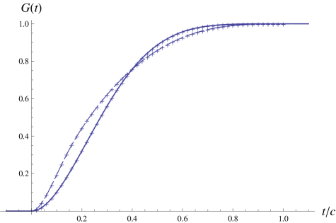
Figure 3: $\mathcal{T}_{a,\;\!a}$ (thick) and $\mathcal{T}_{a,\;\!5a}$ (thin and dashed)

5.2 Two triangles

Fig. 4 shows the density function $cg_{2}$ for $b=5a$, and the corresponding functions $cg_{\mathcal{R}}$ and $cg$. Fig. 5 shows the distribution function $G_{2}$ for $b=5a$, and the corresponding functions $G_{\mathcal{R}}$ and $G$. The plot markers result from a simulation with $c=1$ and $10^{7}$ pairs of random points.

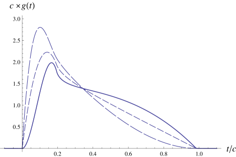
Figure 4: $cg_{\mathcal{R}}$ (short-dashed), $cg$ (long-dashed) and $cg_{2}$ for $b=5a$

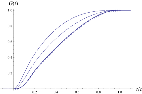
Figure 5: $G_{\mathcal{R}}$ (short-dashed), $G$ (long-dashed) and $G_{2}$ for $b=5a$

References

- [1] Ambartzumjan, R. V.; Mecke, J.; Stoyan, D.: Geometrische Wahrscheinlichkeiten und Stochastische Geometrie, Akademie Verlag, Berlin, 1993.
- [2] Bäsel, U.: Random chords and point distances in regular polygons, arXiv: 1204.2707v2 [math.PR] 5 Sep 2012.
- [3] Borel, E.: Principes et Formules Classiques du Calcul des Probabilités, Gauthier-Villars, Paris, 1925.
- [4] Bronstein, I. N.; Semendjajew, K. A.: Taschenbuch der Mathematik, Verlag Nauka, Moskau und BSB B. G. Teubner Verlagsgesellschaft, Leipzig, 1989.
- [5] Gates, J.: Some properties of chord length distributions, J. Appl. Prob., 24 (1987), 863-874.
- [6] Ghosh, B.: Random distances within a rectangle and between two rectangles, Bull. Calcutta Math. Soc., 43 (1951), 17-24.
- [7] Gille, W.: The chord length distribution of parallelepipeds with their limiting cases, Exp. Techn. Phys., 36 (1988), 197-208.
- [8] Harutyunyan, H. S.; Ohanyan, V. K.: The chord length distribution function for regular polygons, Adv. Appl. Prob. (SGSA), 41 (2009), 358-366.
- [9] Marsaglia, G.; Narasimhan, B. G.; Zaman, A.: The distance between random points in rectangles, Commun. Statist. - Theory Meth., 19(11) (1990), 4199-4212.
- [10] Mathai, A. M.: An Introduction to Geometrical Probability, Gordon and Breach, Australia, 1999.
- [11] Mathai, A. M.; Moschopoulos, P.; Pederzoli, G.: Random points associated with rectangles, Rend. Circ. Mat. Palermo, Serie II, Tomo XLVIII (1999), 163-190.
- [12] Piefke, F.: Beziehungen zwischen der Sehnenlängenverteilung und der Verteilung des Abstandes zweier zufälliger Punkte im Eikörper, Z. Wahrscheinlichkeitstheorie verw. Gebiete, 43 (1978), 129-134.
- [13] Santaló, L. A.: Integral Geometry and Geometric Probability, Addison-Wesley, London, 1976.
- [14] Sulanke, R.: Die Verteilung der Sehnenlängen an ebenen und räumlichen Figuren, Math. Nachr., 23 (1961), 51-74.
- [15] Zhuang, Y.; Pan, J.: A geometrical probability approach to location-critical network performance metrics, INFOCOM, Proceedings IEEE, (2012), 1817-1825.
Uwe Bäsel
HTWK Leipzig, University of Applied Sciences,
Faculty of Mechanical and Energy Engineering,
PF 30 11 66, 04251 Leipzig, Germany,