Modelling the formation of structured deposits at receding contact lines of evaporating solutions and suspensions^†

Ľubor Fraštia,^a Andrew J. Archer,^a and Uwe Thiele ^∗a

Received Xth XXXXXXXXXX 20XX, Accepted Xth XXXXXXXXX 20XX
First published on the web Xth XXXXXXXXXX 200X

DOI: 10.1039/b000000x

When a film of a liquid suspension of nanoparticles or a polymer solution is deposited on a surface, it may dewet from the surface and as the solvent evaporates the solute particles/polymer can be deposited on the surface in regular line patterns. In this paper we explore a hydrodynamic model for the process that is based on a long-wave approximation that predicts the deposition of irregular and regular line patterns. This is due to a self-organised pinning-depinning cycle that resembles a stick-slip motion of the contact line. We present a detailed analysis of how the line pattern properties depend on quantities such as the evaporation rate, the solute concentration, the Péclet number, the chemical potential of the ambient vapour, the disjoining pressure, and the intrinsic viscosity. The results are related to several experiments and to depinning transitions in other soft matter systems.

1 Introduction

Many production processes employed in the chemical, pharmaceutical and other industries, involve a wet phase where films or drops of a solution or suspension are applied to a solid or liquid surface with the aim of producing a homogeneous or structured layer of the solute on the surface. Prominent examples are printing, painting and coating processes where a wet ink or paint is used. The carrier fluid (solvent) then evaporates and leaves all the originally dissolved non-volatile material behind in various deposition patterns on the substrate.

If the aim of these processes is to produce a large-scale homogeneous layer, ideally one would instantaneously produce an extended stable homogenous film of solution that then evaporates slowly and homogeneously. Although, this may be achieved to some extent, e.g. by spin coating, this situation is rather exceptional. In practice, what generally happens is that even while the wet film is still being deposited onto one part of the substrate, it is already dry on other parts. Many techniques exist for applying such films, that are relevant for different surface types and surface geometries, such as painting, blade coating, deposition of individual drops, spray coating, and processes involving liquid menisci.

Historically, the main aim of these processes was to produce homogeneous coatings, so defects like holes or patterned areas would not have been desirable. However, this has changed as nowadays wet deposition may also be used to produce patterned functional layers via the self-organisation of the solute. Although a large variety of different apparatus geometries exists, the basic physical question always is What types of deposition patterns exist and how can the self-organisation processes involved in forming the patterns be controlled? A close inspection of the individual systems shows that in most of them, the formation of deposition patterns occurs in a localised zone at receding contact lines that move under the coupled influence of solvent evaporation, convective motion of the solution, capillarity and wettability.

In this paper we present a long-wave hydrodynamic thin film model that focuses on such a moving contact line. Some of the main features of our model were briefly presented by Frastia et al. ¹. However, before we discuss the model and the wide range of detailed results that we have obtained, we first briefly review some of the relevant experimental systems and theoretical approaches that exist in the literature.

Interest in deposition patterns has markedly increased over the last decade, since Deegan and co-workers’ detailed investigations of the “coffee-stain effect”, i.e., the solute deposition patterns that are left behind by a receding three-phase contact line of an evaporating drop of a suspension upon a smooth solid substrate.^{2, 3, 4} In particular Deegan ³ describes and analyses a wide range of patterns: cellular and lamellar structures, single and multiple rings, and Sierpinski gaskets. The creation of multiple rings through a stick-slip front motion of colloidal liquids was also observed.^{5, 6} Since then, interest widened and now encompasses all phenomena that accompany evaporative and convective dewetting of colloidal suspensions and polymer or macromolecular solutions in a number of different geometries. Other early examples are the investigation by Parisse and Allain of the shape changes that drops of colloidal suspension undergo when they dry ^{7, 8} and the creation of semiconductor nanoparticle rings through a similar deposition process.⁹ Other observed drying structures include crack patterns,¹⁰ chevron patterns,¹¹ and branched patterns.^{12, 13} In fact, crack patterns in sol-gel processes had already been studied somewhat earlier,^{14, 15} however, we do not consider them here. The related concept of using evaporation at contact lines to assemble colloidal particles or proteins into crystals actually has a longer history – see for example the discussions and reviews by Davies et al. ¹⁶, Denkov et al. ¹⁷, Adachi and Nagayama ¹⁸, Maenosono et al. ¹⁹, Kinge et al. ²⁰.

Generally, the evaporation of a macroscopic drop does not usually result in the deposition of regular concentric ring patterns that could potentially be employed to fabricate devices, but rather results in irregular patterns of rugged rings and lines (see, e.g., Adachi et al. ⁵, Deegan ³). This changes when the experiments are performed in a controlled way on smaller scales: Recently, both polymer solutions ^{21, 22, 23} and (nano)particle suspensions ^{24, 25, 26} have been employed in various small-scale geometries where one is able to exercise greater control over the contact line as it recedes due to evaporation. As a result, strikingly regular line patterns are created, where the deposited structures show typical distances ranging from 10–100$\mu$m. Line patterns can be parallel or perpendicular to the receding contact line and are produced in a robust repeatable manner in extended regions of parameter space. Besides the lines, a variety of other patterns may also be found, including undulated stripes, interconnected stripes;²⁵ ladder structures, i.e. superpositions of perpendicular and parallel stripes;²¹ regular arrays of drops;^{27, 21} and irregularly branched structures.^{28, 12, 29, 13} The occurrence of these more complicated patterns is highly sensitive to the particular experimental setup and the system parameters.

Several groups employ this type of wet evaporative deposition as a non-lithographic technique for covering large areas with regular arrays of small-scale structures, such as, e.g., concentric gold rings with potential uses as resonators in advanced optical communications systems ³⁰ or ordered arrays of cyanine dye complex micro-domes employed in photo-functional surfaces.³¹ Often the patterns are robust and can be post-processed, e.g., to create double-mesh structures by crossing and stacking two ladder films.²¹ A number of investigations focus on deposition patterns resulting from more complex fluids, such as phase separating polymer mixtures;³² solutions of DNA,^{33, 34} collagen, ³⁵ liquid crystals,³⁶ dye molecules,^{16, 37, 31} dendrimers,³⁸ carbon nanotubes,^{39, 40} and graphene;⁴¹ and biofluids like blood.^{42, 43} The latter has medical implications as it is thought that one may learn how to detect some illnesses by simple evaporation experiments on small samples.⁴⁴

Surveying the literature, one finds that deposition patterns consisting of regular stripes are a rather generic phenomenon. They occur for many different combinations of substances ⁴⁵ and in a range of different experimental setups that allow for slow evaporation. To better control the contact line motion, various techniques are employed. One may distinguish between passive and active experimental set-ups. In the passive set-up, the solution or suspension is brought onto the substrate and left to evaporate. Examples include (i) the so-called “meniscus technique” (where a meniscus with a contact line is created), e.g., in a sphere-on-flat ^{22, 25, 23} or ring-on-flat ^{17, 46} geometry, (ii) the deposition of a single large drop onto a substrate ^{5, 3} and (iii) the deposition of flat films onto a substrate using spin-coating.^{47, 48} These ‘passive’ set-ups are mainly controlled via the temperature, the partial pressure of the solvent, and the solute concentration.

The active set-ups involve an additional control parameter that can often be better adjusted than those in the passive set-ups. An example is a set-up similar to blade coating where a controlled continuous supply of solution is provided between two glass plates. The upper plate slides backwards with a controlled velocity and in this way maintains a meniscus-like liquid surface where the evaporation takes place and the patterns are deposited.²¹ The deposition patterns are found to depend on the plate velocity. Other examples are a receding meniscus between two glass plates whose receding velocity is controlled by an imposed pressure gradient,²⁶ an evaporating drop that is pushed over a substrate at controlled velocity,²⁴ or a solution that is spread on a substrate by a roller that moves at a defined speed.³¹

Up to this point, we have only mentioned experiments involving evaporating solutions or suspensions on solid substrates. There are two systems that are closely related: On the one hand there exist studies of evaporating films on a fluid substrate, in particular, films of a nanocrystal dispersion in alkanes that spread and evaporate simultaneously on the free surface of a polar organic fluid that is immiscible with the alkane.⁴⁹ The defect-free liquid substrate allows for highly regular periodic stripe patterns that persists over a large area. On the other hand there are many experiments related to the transfer of Langmuir-Blodgett monolayers, i.e., high density surfactant layers, from a trough filled with water onto a solid plate that is withdrawn with a controlled velocity from the bath. Depending, e.g., on the velocity of the plate and the monolayer density on the trough, the transferred monolayer may exhibit stripe patterns parallel or perpendicular to the direction of withdrawal.^{50, 51, 52} We will return to these experiments in the conclusion and discuss in which way our results may be related to these rather different systems.

Despite the large variety of experiments that produce regular line patterns from polymer solutions and colloidal suspensions, a theoretical description of their formation has been rather elusive. Most authors agree that the patterns result from a stick-slip motion of the contact line that is caused by pinning/depinning events.^{3, 30, 22, 53} Various reduced models have been developed that: relate the interaction between the contact line and the deposit that is formed, in terms of a pinning force and derive how this force depends on and scales with the experimental parameters;^{22, 26} develop evolution equations for the shape of an individual deposited ring;³ study the time evolution assuming a permanently pinned contact line.^{54, 55, 56, 57} Hu and Larson ⁵⁸ analytically obtain a flow field that is combined with Brownian dynamics simulations to study particle deposition. Warner et al. ⁵⁹ employs a thin film model similar to the one we present below to describe the dewetting of a film of a nanoparticle suspension. They study the regime where drop arrays form via directed convective dewetting of the solvent before they subsequently dry out. A thin film model that produces rings is presented by Kaya et al. ⁶⁰, however, there the contact line is shifted ‘by hand’ if a certain condition is met. A thin film description of an evaporating drop of a suspension may also be coupled to a full description of the diffusion of vapour in the gas phase.⁶¹ This model is used to predict the dependence of the mean deposit thickness on the substrate velocity, but is not used to describe the formation of deposition patterns.

In another approach, the system is described using a complex non-isothermal Navier–Stokes model, i.e., with the complete set of transport equations for momentum, energy, and solute and vapour concentration, thereby incorporating evaporation, thermal Marangoni forces and rules for contact line motion.⁵³ Bhardwaj et al. ⁶² further incorporate Derjaguin–Landau–Verwey–Overbeek (DLVO) interactions between solute particles and the solid substrate in the form of effective forces in the advection-diffusion equation for the solute concentration. Simulations show the formation of and depinning from a single deposit line, but for the parameter values used in this study, they do not observe periodic deposits.⁵³

To our knowledge, there exists no efficient model that is able to capture the dynamics of the periodic deposition process, i.e., the stick-slip character of the process. By ‘efficient’ we mean a model that allows for a numerical exploration of the parameter space. The full transport equations contain all or most of the physics, however, they are tedious to use and tricky when it comes to incorporating details like the wettability and contact line motion. Models that assume a pinned contact line are only able to describe how a deposit forms for a fixed drop base, even if they are fully dynamic thin film models. For instance, the model by Okuzono et al. ⁵⁵ distinguishes a fluid and a gel-like part of the drop and allows one to follow the time evolution of the drop and concentration profiles. It can distinguish between final deposits of basin-, crater-, and mound-type. The crater-type deposits might be seen as resulting from the deposition of a single ring. However, models like this one that fix the drop base are not able to capture the deposition of multiple rings or of a regular line pattern in planar geometry. Note also that a first fully dynamic model exists for the related phenomenon of the transfer of Langmuir–Blodgett surfactant monolayers from a bath onto a solid substrate.⁶³ There, the stripe formation is related to a phase transition in the surfactant layer that results from a substrate-mediated condensation effect. We discuss similarities and differences of the model by Köpf et al. ⁶³ and our thin film model for a receding contact line of an evaporating solution in section 2.

The aim of the present work is to analyse in detail the results from a dynamic close-to-equilibrium thin film model that allows for a generic description of a receding contact line of a solution in the passive geometry, i.e., without an externally imposed velocity. We show that the model is able to capture the dynamics of the stick-slip motion of the receding three-phase contact line of a colloidal suspension or polymer solution on a solid substrate. For a range of parameter values, as the solvent evaporates, the model predicts the deposition of regular and irregular patterns of lines that are parallel to the receding contact line. The model allows us to elucidate generic mechanisms that play an important role in many of the experimental systems that are studied. Furthermore, we are able to determine the influence of varying the basic model parameters on the deposition patterns, in particular, on the spatial period, amplitude, and morphology of the deposited lines. In the present work we restrict our attention to one-dimensional deposition patterns, i.e., regular and irregular line patterns. The limitations of this approach are discussed in the conclusion.

This paper is laid out as follows: In Section 2 the thin film model is introduced in the form of evolution equations for the film thickness and concentration profile, that are obtained from making a long-wave approximation. The model is discussed in the context of related models in the literature. In Section 3, results from time simulations are presented. It is shown that solely having a viscosity that diverges at a critical solute concentration is sufficient to trigger a self-organised periodic pinning-depinning process that results in the deposition of regular line patterns in a well defined region of the parameter space spanned by our non-dimensional control parameters, i.e., evaporation rate, mean solute concentration, Péclet number, parameters related to wettability, solvent vapour chemical potential, and the intrinsic viscosity. The final Section 4 gives our conclusions and an outlook on future work. Two appendices discuss details of our numerical scheme (Appendix A) and the measures we use to quantify the obtained line patterns (Appendix B), respectively.

2 The thin film model

Fig.  1: Diagram showing a liquid front that recedes due to evaporation and convection. The front has varying velocity $v(t)$ and the liquid film thickness profile is given by the function $h(x,t)$. In the bulk film the profile $c(x,t)$ is the vertically averaged solute concentration profile and outside the liquid film, the solute layer thickness is given by ${h_{\mathrm{p}}}(x,t)=c(x,t)h(x,t)$.

We consider a thin film of an evaporating partially wetting nanoparticle suspension (or polymer solution) on a flat solid substrate in contact with its vapour (see Fig. 1). We assume that the densities of the solvent and solute are matched, so there is little or no sedimentation of the solute within the solvent, and slow evaporation so that we may neglect the dependence on the vertical coordinate of the solute concentration within the liquid film. Assuming that all surface slopes are small, one may employ a long-wave approximation ^{64, 65} and derive two coupled evolution equations for the film thickness profile $h(x,t)$ and the concentration of the solute $c(x,t)$, which can be written in compact form as a pair of continuity equations for the solution and the solute, respectively:

$$\partial_{t}h =-\partial_{x}j_{\mathrm{c}}(h,c)-j_{\mathrm{e}}(h),$$ (1)

$$\partial_{t}(ch) =-\partial_{x}\left[cj_{\mathrm{c}}(h,c)+j_{\mathrm{d}}(h,c)\right],$$ (2)

The equation for the solution, i.e., the film thickness evolution equation (1), contains a non-conserved evaporative source term and a conserved convective transport term. The equation for the solute i.e., the evolution equation (2) for the effective solute layer thickness ${h_{\mathrm{p}}}=ch$ only has a conserved dynamics, which is made up of two terms: the first is a convective transport term and the second describes transport due to diffusion. These coupled convective, evaporative, and diffusive fluxes are given by

$$j_{\mathrm{c}}(h,c) =-Q_{\mathrm{c}}(h,c)\partial_{x}p(h)=-\frac{h^{3}}{3\eta(c)}\partial_{x}p(h),$$ (3)

$$j_{\mathrm{e}}(h) =\frac{\beta}{\rho}\left[p(h)-\mu\rho\right],$$ (4)

$$j_{\mathrm{d}}(h,c) =-Q_{\mathrm{d}}(h,c)\partial_{x}c=-D(c)h\partial_{x}c.$$ (5)

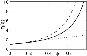
Fig.  2: Dependence of the viscosity on the scaled solute concentration $\phi=c/c_{\mathrm{c}}$, as described by the dimensionless form of the Krieger–Dougherty law in Eq. (16). The solid line is for the exponent $\nu=1.575$, whereas the dashed one is for $\nu=2$. The linear Einstein relation is given as dotted line.

The first term on the right hand side of Eq. (1) is the conserved part of the dynamics, where $j_{\mathrm{c}}$ [given in Eq. (3)] is the total horizontal volume flux (integrated over film thickness). This flux is driven by the pressure gradient. The pressure $p$ is discussed below. The convective mobility function $Q_{\mathrm{c}}(h,c)=h^{3}/3\eta(c)$ in $j_{\mathrm{c}}$ [Eq. (3)] results from the Poiseuille flow of the liquid in the case of a no-slip boundary condition at the substrate and the free upper surface. The dynamic viscosity, $\eta(c)$, exhibits a strong nonlinear dependence on the local solute concentration and obeys the Krieger–Dougherty law ^{66, 67}

$$\eta(c)=\eta_{0}\,\left(1-\frac{c}{c_{\mathrm{c}}}\right)^{-\nu},$$ (6)

where $\eta_{0}$ is the dynamic viscosity of the pure solvent. Note that the solute bulk concentration field $c(x,t)$ is a dimensionless volume fraction concentration and $c_{\mathrm{c}}$ is the critical value at random close packing, where the viscosity diverges, i.e. $\eta(c)\to\infty$ when $c\to c_{\mathrm{c}}^{-}$. For hard-spheres $c_{\mathrm{c}}=0.63$. The viscosity concentration dependency Eq. (6) is illustrated in Fig. 2.

In general, the precise value of the exponent $\nu$ depends on the type of suspension employed. Here we mainly consider particles that have no net attractive forces between them and only have excluded volume interactions, i.e., they interact via a hard-core repulsion when coming into direct contact. For such particles, values for $\nu$ between 1.4 and 3 are discussed in the literature, depending on their shape.⁶⁶ The exponent $\nu$ is sometimes written as $\nu=[\eta]c_{\mathrm{c}}$, where $[\eta]$ is the intrinsic viscosity, see,Larson ⁶⁶ defined by

$$[\eta]=\lim_{c\rightarrow 0}\frac{\eta-\eta_{0}}{\eta_{0}c}.$$ (7)

For spherical particles $[\eta]=2.5$, resulting in $\nu=1.575$. Other thin film models use $\nu=2$.^{68, 59} For solute particles with net attractive forces between them, values for $\nu$ as low as 0.13 are reported.⁶⁹ Depending on the particular system, the transition at $c_{\mathrm{c}}$ is either referred to as jamming or gelation.^{69, 55} Here we fix $\nu=1.575$, corresponding to particles that only interact via excluded volume interactions, in order to gain an understanding of these types of systems and also to determine the regions of qualitatively different behaviour in the phase plane spanned by the evaporation rate and concentration, defined below. Additional investigations show (see Section 3.7) that the formation of periodic deposits is somewhat more pronounced for smaller $\nu$, which corresponds to more strongly attracting solute particles.

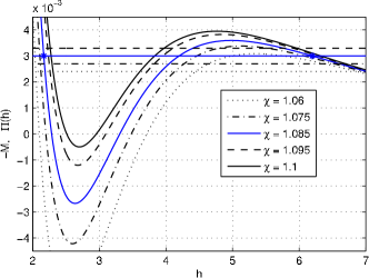
Fig.  3: (Color online) The non-dimensional disjoining pressure $\varPi(h)$, given in Eq. (15), for various values of $\chi$, as given in the legend. The horizontal straight lines indicate various values of the non-dimensional chemical potential $M$, given in Eq. (19). The blue solid lines for the disjoining pressure and chemical potential correspond to our ‘standard’ values of $\chi=1.085$ and $M=-0.003$, respectively (see the end of Section 2). The other lines correspond to parameter values employed in Section 3.6 below. The blue stars denote the stable film heights: $h_{1}<h_{2}$ for the standard values.

The convective flow is driven by the gradient of the pressure

$$p(h)=-\gamma\partial_{xx}h-\varPi(h),$$ (8)

where the first term is the Laplace pressure ($\gamma$ is the surface tension) and the second term is the disjoining (or Derjaguin) pressure

$$\varPi(h)=\frac{2S^{\mathrm{LW}}d_{0}^{2}}{h^{3}}+\frac{S^{\mathrm{P}}}{l_{0}}\exp\frac{d_{0}-h}{l_{0}}$$ (9)

that models wettability effects for a partially wetting fluid;^{70, 71, 65} see Fig. 3 for a graphical representation of its non-dimensional form. $l_{0}$ is the Debye length, $d_{0}$ is a molecular interaction length, $S^{\mathrm{LW}}=-A/12\pi d_{0}^{2}$ and $S^{\mathrm{P}}<0$ are the apolar and polar spreading coefficient, respectively, and $A<0$ is the Hamaker constant. We expect qualitatively similar behaviour for other combinations of stabilising and destabilizing terms in $\varPi(h)$.^{72, 73, 74}

The second term on the r.h.s. of Eq (1) represents the non-conserved part of the dynamics and models evaporation, where $j_{\mathrm{e}}$ [given in Eq. (4)] is the evaporative flux density at the free surface of the film. Here, we assume that the system is close to equilibrium and that the vapour is near to saturation and so evaporation is slow. In this limit evaporation with a rate $\beta$ is driven by the difference of the scaled pressure $p/\rho$ and the chemical potential of the ambient vapour $\mu$.^{75, 76} Latent heat effects may be neglected, and the density $\rho$ is assumed to be equal for the solute particles and the solvent.

The first and second terms on the right hand side of Eq. (2) model convective and diffusive transport of the solute, respectively. Since the solute is passively advected by the fluid, the convective flux is given by $cj_{\mathrm{c}}$. For the diffusive flux [given in Eq. (5)] we assume Fick’s law and we set the diffusive mobility to be $Q_{\mathrm{d}}(h,c)=D(c)h$, where $D(c)$ is the concentration dependent diffusion coefficient, and we employ the Einstein–Stokes relation

$$D(c)=\frac{k_{B}T}{6\pi r_{0}\eta(c)},$$ (10)

where $k_{B}$ is the Boltzmann constant, $T$ the temperature, and $r_{0}$ the solute particle radius.

To facilitate a comparison of our results with the literature we employ a scaling identical to that employed by Lyushnin et al. ⁷⁵ and,Frastia et al. ¹ namely: time, horizontal $x$-coordinate, and film thickness scales are

$$\tau =\frac{3\eta_{0}\gamma}{\delta|\widetilde{S}^{\mathrm{P}}|^{2}},\qquad\alpha=\left(\frac{\delta\gamma}{|\widetilde{S}^{\mathrm{P}}|}\right)^{1/2},$$

$$\mbox{and}\qquad\delta =\left(\frac{A}{6\pi|\widetilde{S}^{\mathrm{P}}|}\right)^{1/3},$$ (11)

respectively, where

$$\widetilde{S}^{\mathrm{P}}=\frac{S^{\mathrm{P}}}{l_{0}}\exp\frac{d_{0}}{l_{0}}.$$ (12)

Using this scaling, Eqs. (1) and (2) are brought into the following non-dimensional form

$$\partial_{t}h =\partial_{x}\left[\frac{h^{3}}{\eta(\phi)}\partial_{x}p(h)\right]-\varOmega_{0}\left[p(h)-M\right],$$ (13)

$$\partial_{t}(\phi h) =\partial_{x}\left[\frac{\phi h^{3}}{\eta(\phi)}\partial_{x}p(h)\right]+\partial_{x}\left[\frac{h}{\mathrm{Pe}\,\eta(\phi)}\partial_{x}\phi\right],$$ (14)

where

$$p(h)=-\partial_{xx}h-\varPi(h)=-\partial_{xx}h-h^{-3}+\exp(-\chi h).$$ (15)

Note that starting with Eqs. (13) and (14) in the remainder of the paper, the symbols $h$, ${h_{\mathrm{p}}}$, $t$, $x$, $p$, $\eta$, and $\varPi(h)$ stand for the non-dimensional quantities whereas up to this point they denoted the dimensional quantities. However, for the scaled concentration we introduce $\phi=c/c_{\mathrm{c}}$. The diffusion coefficient is expressed as $\left[\mathrm{Pe}\,\eta(\phi)\right]^{-1}$, where $\mathrm{Pe}$ is the Péclet number and the dimensionless viscosity function is

$$\eta(\phi)=(1-\phi)^{-\nu}.$$ (16)

The dimensionless numbers in Eqs. (13)–(15) are defined as

$$\chi =\left(\frac{|A|}{6\pi|\widetilde{S}^{\mathrm{P}}|l_{0}^{3}}\right)^{1/3},$$ (17)

$$\varOmega_{0} =\frac{18\pi\beta\eta_{0}\gamma}{\rho\left[6\pi A^{2}|\widetilde{S}^{\mathrm{P}}|\right]^{1/3}},$$ (18)

$$M =\frac{\rho\mu}{|\widetilde{S}^{\mathrm{P}}|},$$ (19)

$$\mathrm{Pe}^{-1} =\frac{3k_{B}T}{r_{0}\left[6\pi A^{2}|\widetilde{S}^{\mathrm{P}}|\right]^{1/3}},$$ (20)

where the evaporation number, $\varOmega_{0}$, is the ratio of the time scales of convection and evaporation of a film without solute and the reciprocal Péclet number, $\mathrm{Pe}^{-1}$, is the ratio of the time scales of convection and diffusion.

There exist a number of models in the literature that are similar to that defined in Eqs. (13) and (14). One is used to study macroscopic particle-laden film flow down an incline.⁶⁸ There, the solvent is non-volatile and changes in the particle concentration result from the settling of particles due to gravity. As the particles in the model of Cook et al. ⁶⁸ are assumed to be large, no diffusion is included in the model, nor is wettability; the advancing of the contact line is facilitated by a precursor film of imposed height. Another example is the case of a surface-passive solute studied by Warner et al. ⁵⁹ [their Eqs. (54) and (55)]. They use a different Derjaguin pressure that, however, also models partially wetting liquids. The main difference is in the evaporation model that they use, which incorporates a vapour recoil effect. They also model particle diffusion in a manner that is independent of solute concentration. Both, Cook et al. ⁶⁸ and Warner et al. ⁵⁹ use a Krieger–Dougherty law to model the dependence of the viscosity on the concentration. This is also done by Craster et al. ⁷⁷ where the spreading and retraction of evaporating droplets containing nanoparticles is studied with a thin film model that involves a structural disjoining pressure. There are some similarities to other models ^{54, 55, 57} where, however, the contact lines are kept pinned. Since moving contact lines are an intrinsic part of the solute deposition process that we study here, we do not refer any more to these other approaches.

The evaporation model that we use is valid close to equilibrium where the film may be considered isothermal. The evaporation is limited by the kinetics of the phase transition (or by the boundary layer transfer, but not by the diffusion of solvent vapour in the gas phase) in the contact line region, which is influenced by the effective molecular interactions, i.e., the saturated vapour pressure depends on the disjoining pressure and curvature in the manner employed in studies of evaporating films and drops.^{75, 78, 76, 74, 79} Our evolution equation (13) reduces to the model by,Lyushnin et al. ⁷⁵ in the limit $\phi_{0}\to 0$. Note, that one may also obtain our evaporation model by taking the isothermal limit of the models by.Ajaev ⁸⁰, Rednikov and Colinet ⁸¹ For a further discussion see.Todorova et al. ⁷⁹

In the present work, we restrict our attention to line patterns deposited through evaporative dewetting, i.e., we assume a one-dimensional geometry, as sketched in Fig. 1. It is known from the experiments that line patterns are not always transversally stable. We discuss this point in relation to our results in the conclusion. We start our numerical computations with an initial condition that corresponds to a spatially one-dimensional semi-infinitely extended film of constant thickness that is connected to a thin precursor layer. The thickness of the precursor film corresponds to the equilibrium height where the Derjaguin pressure and evaporation balance. The liquid in the film is a suspension with a constant solute concentration. We discretize the non-dimensional equations (13) and (14) over a finite domain $x\in[0,L]$ where the dewetting front is located close to the boundary of the domain at $x=0$, see Fig. 1. The details of the implementation including the procedure we use for shifting the spatial computational domain at certain times are given in Appendix A.

Initially, we employ a set of values of our dimensionless parameters that we will refer to as the standard configuration: We set the dimensionless chemical potential, $M=-0.003$, and the dimensionless disjoining pressure parameter $\chi=1.085$, which are the same values as used by.Lyushnin et al. ⁷⁵ The other parameters are modified to accommodate the effect of the solute. In particular, for the initial results presented here, we use the evaporation rate $\varOmega_{0}=4.64\times 10^{-7}$; the scaled constant bulk concentration, $\phi_{0}=0.41$, that enters the simulation as a given initial value; the reciprocal Péclet number, $\mathrm{Pe}^{-1}=0.0003$; and the exponent of the Krieger–Dougherty law, $\nu=1.575$, as discussed above after Eq. (7).

The main control parameters in our simulations are $\varOmega_{0}$ and $\phi_{0}$. These two parameters span the plane within which we determine regions where periodic patterns and other characteristic deposits occur. Then, for selected fixed parameter combinations $(\varOmega_{0},\phi_{0})$, we vary one of the parameters $\mathrm{Pe}^{-1}$, $M$, $\chi$, and $\nu$ while the remaining parameters are kept fixed, in order to determine how sensitive the behaviour of the system is to variations in the value of these.

3 Results

3.1 Dynamics of the evaporative dewetting front

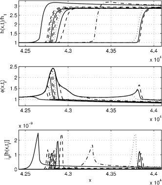
Fig.  4: Sequences of snapshots of film thickness profile $h(x,t)$ (top panel), mean concentration $\phi(x,t)$ (middle), and evaporation flux $j_{\mathrm{e}}(x,t)$ (bottom), which illustrate the pinning-depinning dynamics. The individual profiles in each sequence are plotted starting at the same time, with a time-increment $\Delta t=10^{9}$ between each successive curve, and are displayed with periodically repeated line styles (solid, dashed, dash-dotted, dotted, solid, …). All the model parameters are set to the ‘standard values’, which are defined at the end of Sec. 2.

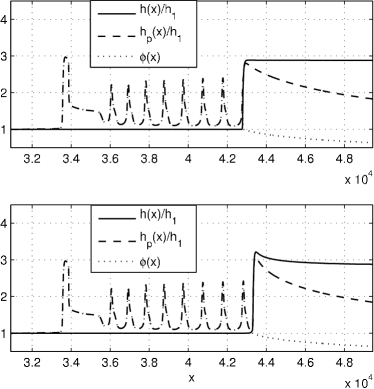
Fig.  5: Snapshots from the deposition process at two characteristic stages: evaporation-dominant (top) and convection-dominant (bottom). The system parameters are as in Fig. 4. The profiles in the top and bottom panel correspond to the 4th and the 11th profile in time in Fig. 4, respectively. Note the capillary ridge behind the front in the lower plot, which is absent in the upper evaporation-dominated stage of the cycle.

Fig.  6: (Color online) Space-time plots of the nanoparticle deposit thickness ${h_{\mathrm{p}}}(x,t)$ (top) for the standard values of the system parameters, where the deposited lines have characteristic heavy right tail (see Fig. 11) and a contour plot of the film height $h(x,t)$ (bottom) in the rectangular region marked in the upper plot. There are 24 equally spaced level contours in the interval of heights $[1.2,3.25]$ which allows the steep dewetting front and capillary ridges to be resolved.

Fig.  7: (Color online) Space-time plots of the nanoparticle film height ${h_{\mathrm{p}}}(x,t)$ for 2 characteristic cases: the upper panel shows deposit lines with a dominant left ‘tail’ ($\varOmega_{0}=4.64\times 10^{-6}$, other parameters are standard). The regular line pattern corresponding to this situation is shown in Fig. 11. The lower panel shows a long-period large-amplitude pattern ($\phi_{0}=0.31$, other parameters are standard). A regular line pattern for the close, but slightly different value $\phi_{0}=0.3016$ is shown in Fig. 11.

Our investigations are mainly based on time simulations of the front motion and the deposition process. We start with a semi-infinitely extended liquid film that coexists with an ultrathin precursor film. The initial dewetting front has a step-wise profile, but is smoothed by capillarity during the very first time steps. The concentration is initially set to a uniform value $\phi(x,0)=\phi_{0}$. The chosen value of the vapour chemical potential ensures that the front recedes by evaporation and/or convection. As the front recedes, it deposits part of the solute in an initially smooth layer. Then, in most cases, the front settles after some transient into a different type of regular motion.

The time-dependent behaviour of the system is well known in the case without solute $(\phi_{0}=0)$.⁷⁵ There, the front profile always converges to a constant shape that moves with constant velocity, i.e., the front motion is stationary. In this situation, one may still distinguish between two qualitatively different limiting cases: (i) convection-dominated and (ii) evaporation-dominated dewetting. They are found for small and large values of the evaporation number $\varOmega_{0}$, respectively. In case (i) the convective motion maintains a capillary ridge despite the ongoing evaporation whereas in case (ii) convection is much slower than evaporation and there is no capillary ridge.

In the presence of a solute, the situation is more complex and there exist extended regions in parameter space where no stationary front motion is found. Instead, the receding front shows an unsteady motion with periodically changing front velocity and shape. An example of such a dynamics is shown in Figs. 4, 5 and 6. These figures illustrate various aspects of the periodic pinning-depinning dynamics of the front that is related to a periodic transition between evaporation- and convection-dominated regimes of the front motion. Fig. 4 shows snapshots of the film height $h(x,t_{i})$, concentration $\phi(x,t_{i})$ and evaporation flux $j_{\mathrm{e}}(x,t_{i})$ profiles. They are equidistant in time and cover just over one period in time. The pinned (evaporation-dominated) regime is characterised by densely spaced profiles when the front is at about $x=4.275$. During this stage the front moves very slowly, the height profile has no capillary ridge and the evaporative flux is rather localised. In contrast, during the depinned (convection-dominated) stage of the cycle, the profiles are sparsely distributed (i.e., the front is fast), the convective motion supplies enough solution to maintain a capillary ridge and therefore the evaporative flux is spread over a wider $x$-region. Note that the maximal $j_{\mathrm{e}}(x,t)$ is actually larger during the depinned regime.

Transitions between the two regimes can be explained as follows: In the early stage of the convection-dominant phase the front moves relatively fast, although the evaporation flux, $j_{\mathrm{e}}(x,t)$, is still greatest in the contact line region. This results in an increase of the local concentration $\phi(x,t)$ and, in consequence, in a strongly nonlinear increase of the viscosity in this region that suppresses the convective motion of the front. As a result, the front slows down and if the local solute concentration reaches random close packing ($\phi(x,t)\to 1$) the convective motion in the contact region stops completely. Thus, the suspension becomes locally jammed. In the case of a polymer solution the transition may be referred to as a local gelling transition (as employed, e.g., in the piece-wise model by.Okuzono et al. ⁵⁵) With the convective motion arrested, the front only moves by evaporation. As the resulting front velocity can be orders of magnitude slower than during the convective motion; the front seems to be pinned. This is clearly visible in the space-time plots of Figs. 6 and 7. The typical front shape at this stage is then monotonic, and no capillary ridge exists [see the solid line in Fig. 5(a)]. During this phase of slow evaporative motion, the front effectively leaves deposits of the highly concentrated solute. As a result, the concentration and therefore viscosity in the contact line region decrease, allowing the convective motion to start again. The front speed is then much larger than in the evaporation-dominated phase, and the front seems to depin. The typical front shape at this stage is non-monotonic, due to the presence of a capillary ridge [see the solid line in Fig. 5(b)]. Note that the width of the region at the front where the concentration of the solute is locally increased varies over time. The extent (along the $x$-axis) of this region is visible in Fig. 7 as the bright (white) region of the field ${h_{\mathrm{p}}}(x,t)$ at the receding dewetting front. We see that in the convective regime the width increases as the solute gets concentrated and in the evaporative (pinned) regime the width decreases as the solute is deposited and left behind the front.

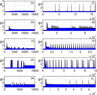
Fig.  8: (Color online) A selection of typical deposit profiles, including the spatial region where the transient to long-time behaviour occurs. The panels show deposition of (a) no lines (but in the transient stage ${h_{\mathrm{p}}}$ may change nonmonotonically); (b) a single line followed by a flat layer; (c) transient lines (whose amplitude decays first fast then slow) followed by a flat layer; (d) transient lines (whose amplitude decays first slow then fast) followed by a flat layer (decreased $\nu=1.25$); (e) an intermittent line pattern [which is a magnification of the pattern in panel (g)]; (f) transient double lines (converging to regular lines); (g) an intermittent line pattern; (h) transient lines followed by a regular line pattern; (i) transient lines converging to a regular pattern of double lines (decreased $\chi=1.065$); (j) a long-period pattern switching between a flat layer and a single line with a leading depression (decreased $\nu=1.25$). The corresponding parameters for (a–j) are: $\varOmega_{0}=($4.64, 14.68, 4.64, 0.167, 0.147, 0.464, 0.147, 0.464, 0.7, 0.464)$\times 10^{-6}$, $\phi_{0}=($0.3343, 0.41, 0.3588, 0.41, 0.41, 0.2983, 0.41, 0.41, 0.41, 0.498). The remaining parameters are the standard values, defined in section 2. The letters (a-d, g, h) are used to mark the corresponding regions in the phase diagram displayed in Fig. 9.

The resulting periodic pinning-depinning cycle – that is perceived as a stick-slip motion – can be best appreciated in the space-time plot displayed in Fig. 6(b) which shows the film thickness profile. The contours of $h(x,t)$ in the steep dewetting front region are so closely bunched that they appear to be a single thick line whose slope, ${\mskip 1.0mu minus 1.0mu\mathrm{d}}x/{\mskip 1.0mu minus 1.0mu\mathrm{d}}t$, corresponds to the velocity of the dewetting front. It is clearly visible that the velocity periodically changes between two rather different values. Further contour lines to the right of the moving front show the periodic appearance of a capillary ridge in the phases of convective motion. The pinning-depinning cycle can also be seen in the space-time plots of the effective nanoparticle layer thickness ${h_{\mathrm{p}}}(x,t)$ presented in Fig. 6(a) and 7. There, however, the capillary ridges are not as clearly visible because ${h_{\mathrm{p}}}(x,t)$ decreases faster when moving away from the dewetting front into the wet region.

The significant changes in the relative importance of convective and evaporative fluxes can be conveniently described by a local evaporation number $\varOmega_{\mathrm{loc}}=(\eta(\phi)/\eta_{0})\varOmega_{0}$. When $\varOmega_{\mathrm{loc}}$ diverges, the front seems pinned, but actually still moves extremely slowly by evaporation alone, and deposits a line or a thick layer of solute. When $\varOmega_{\mathrm{loc}}$ sufficiently decreases, the front depins and convective motion resumes.

We use the simulation set up described above to investigate the transient and long-time deposition behaviour. It is found that after the initial transient (that may involve the deposition of some irregular lines) various scenarios are possible, depending on the values of our model control parameters. Most importantly, there exists an extended region in parameter space, where after a transient, very regular line patterns are deposited (see Figs. 5, 6 and 7). In these cases the pinning-depinning process is repeated in a regular manner. Particular features of the deposited pattern depend on the particular values of the model parameters and are discussed below. The occurrence of periodic deposits for an extended parameter range indicates that this phenomenon is robust and explains why the deposition of line patterns is found in a wide variety of experimental settings with various suspensions and solutions, where it is often described as resulting from a regular stick-slip motion of the contact line.^{30, 22, 26}

Before we discuss the various types of deposition patterns that we observe as the system parameters are varied, we return to the space-time plots in Figs. 6 and 7 that already indicate how the ratio of typical time scales for the convection- and evaporation-dominated front motion changes with increasing evaporation number and mean concentration. Fig. 6 shows (as do Figs. 4 and 5) our standard case (described at the end of Sec. 2). There, the ratio of the velocities of the dewetting front in the depinned and pinned regime is $45.07$. Increasing the evaporation rate coefficient to $\varOmega_{0}=4.64\times 10^{-6}$ (keeping the other parameters at the standard values), the evaporative flux becomes stronger and the convective motion is not fast enough to create a large capillary ridge. As a result, the difference between the depinned and pinned regimes is smaller and so the ratio of the velocities decreases to $8.16$ [see Fig. 7(a)]. Further increasing of $\varOmega_{0}$ eventually results in the deposition of a layer of constant thickness. If instead one decreases the concentration to $\phi_{0}=0.31$ (keeping the other parameters at standard values), see Fig. 7(b), the viscosity in the convective regime decreases and the capillary ridges become larger. Because there is less solute present, it takes longer to build up a high concentration of solute in the contact line region and to pin the front. This results in an increased length of the convective phase of the cycle (compare Figs. 7(b) and 6) and to an increase of the ratio of velocities to $80.36$. A further decrease in the concentration prolongs the convective phase even more until eventually the length of the convective phase diverges (at finite concentration value, see below).

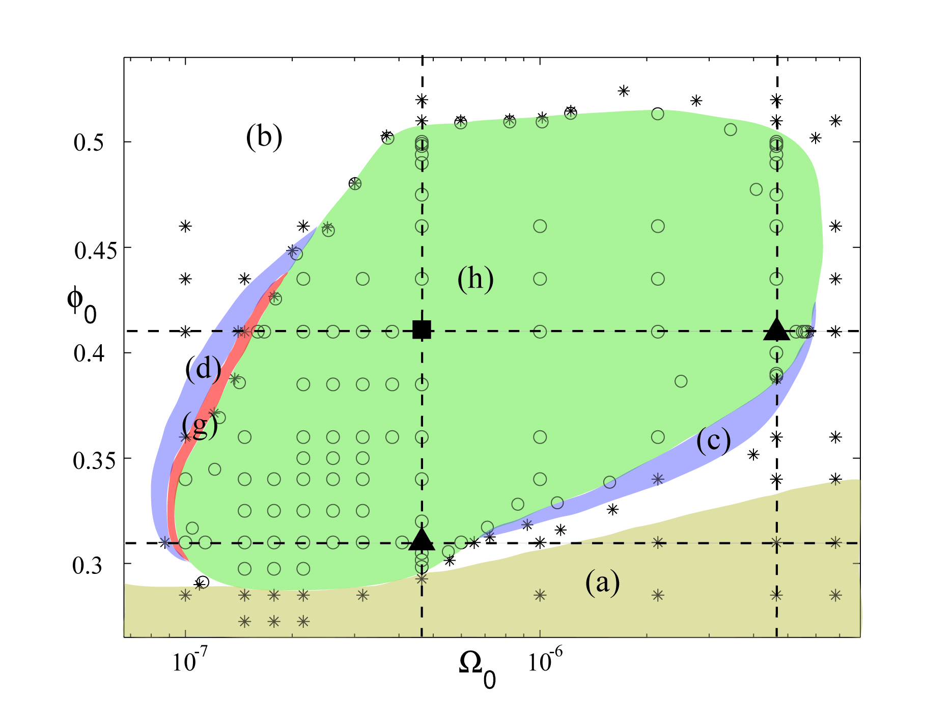
Fig.  9: (Color online) Morphological phase diagram of deposition patterns, in the plane spanned by the evaporation number $\varOmega_{0}$ and the bulk concentration $\phi_{0}$. Letters (a)-(d), (g) and (h) in the differently shaded areas (coloured online) indicate the type of pattern that is found there using the same letters as in the caption of Fig. 8. In particular, in the central grey area (green online) regular line patterns are found after some transient (simulations denoted by $\circ$), while outside this area (simulations denoted by $\ast$) a layer of constant height is deposited after a variety of transients indicated by subregions of different shading (colour online). As an exception, an intermittent pattern is found in the small (red online) region (g). Results obtained along the dashed vertical and horizontal lines are presented in subsequent figures and discussed in detail in the main text. The standard configuration defined at the end of Section 2 and shown in Figs. 4 to 6, is marked by the small filled square where the left vertical and upper horizontal dashed lines cross. Fig. 7 gives results for the two other crossing points that are marked by filled triangles.

3.2 Types of deposition patterns

An extensive parameter scan in the space spanned by our control parameters – $\varOmega_{0}$, $\phi_{0}$, $\mathrm{Pe}^{-1}$, $\chi$, $M$, and $\nu$ – reveals a zoo of various different deposition patterns and allows one to study the dependence of the pattern morphology on the control parameters. An overview of typical deposit profiles, $\phi(x)$, is displayed in Fig. 8. The letters (a)–(j) that indicate the individual panels are used in the following list that describes important properties of the individual patterns. They are also used to indicate the corresponding regions in the morphological phase diagram in Fig. 9.

• After a short transient during which the height of the deposit can vary nonmonotonically (there can be a very small bump but the solution is not in jammed state), a layer of constant thickness is left behind the moving front. This is normally observed for very dilute solutions at any evaporation number. The solute concentration in the resulting film is everywhere below the jamming threshold, i.e. the solute may still diffuse within the precursor film. This is in contrast to all the other cases where at least parts of the deposit (normally the lines) are in the jammed state.

• A single line is deposited as the final part of a long initial transient before a flat layer is deposited. This represents the case closest to the original coffee stain effect where a single ring is deposited from an evaporating droplet. This behaviour is observed for a wide parameter range outside the region of periodic patterns [see (h) below] and for denser solutions than in case (a). Apart from in the region of the initial line deposit, the solute in the flat layer is not necessarily jammed.

• A finite number of lines is deposited as part of a long initial transient before a flat layer of solute is deposited. This represents the experimental case where multiple irregular rings are deposited from an evaporating droplet. This behaviour occurs in bands around the region of periodic patterns. Panels (c) and (d) in Fig. 8 present deposit profiles from the regions with higher and lower $\varOmega_{0}$ than in the periodic line region (cf. Fig. 9), respectively.

• A very long transient of a periodic pattern of double lines. The pattern slowly evolves towards one with regularly spaced lines by slowly changing the distance between the two lines in the respective pairs. The initial transient deposit is a flat layer and the size and shape of the first line is not significantly different from the following lines. This pattern is observed for very low solute concentrations and for somewhat small evaporation rates in the region of periodic lines close to its boundary.

• An intermittent pattern (a magnification of a portion of this is displayed in Fig. 8(e)). A rather irregular line pattern is deposited in an intermittent manner, i.e., there are times when a nearly flat layer is left behind the front which alternate in a non-periodic way with episodes where line patterns are deposited. These line patterns are not periodic but exhibit a typical timescale; see the magnification in Fig. 8(e). This behaviour is found in a very narrow band between the region of periodic patterns and the band where single or multiple lines form (cf. Fig. 9).

• After a short monotonous transient, the deposition of lines starts with a large first line followed by a small number of transient lines. The transient lines in Fig. 8(h) are of increasing period, however, the case of decreasing period is also observed. The line deposition rapidly converges to a regular periodic state. For instance, Fig. 8(h) shows a case where a rather high initial line terminates in a shoulder that is then followed by lower lines that slowly increase in height and converge to the truly periodic line pattern. This profile is at the standard values of our control parameters; see also the results in Figs. 5 and 6. This behaviour is found in a large region of the space spanned by our main control parameters (Fig. 9). The region may shrink and disappear if other parameters are strongly changed away from their standard values, such as, e.g. increasing the diffusion coefficient leads to the pattern formation being suppressed (see section 3.5).

• Stable double lines can be observed for values of the parameter $\chi$ in the disjoining pressure that are less than our standard value. For the case displayed in Fig. 8(i), we observe that a large initial line is deposited followed by some irregular lines with monotonically increasing line distance. However, unlike the transient double lines in case (f), here the distances adjust till a regular pattern of double lines is deposited in a stable manner.

• After the initial transient deposition of a finite number of lines it at first seems that a region of flat film follows. However, the flat film actually becomes a long-period pattern that switches between a flat layer and single lines with a leading depression. This pattern was observed for a lower value of the viscosity exponent, $\nu=1.25$, that corresponds, e.g., to a suspension of non-spherical particles. A similar pattern was observed at the boundary of region (h), where $\phi_{0}=0.31$ and $\varOmega_{0}$ is small. In this case, switching between a flat layer and multiple lines occur.

Note, that in some cases where the concentration is small, the concentration in the ‘valleys’ between the periodic lines is sufficiently low that the solution is not jammed in these regions; an example is given in Fig. 8(f).

As our parameter space is 6 dimensional and the equations of the model (13) and (14) are highly nonlinear, our list of typical patterns must certainly be incomplete. As our investigation is numerical in nature, we are unable to determine to which state some of the very long initial transients converge. Below, we discuss the various transitions between the observed patterns on changing a control parameter. This allows us to speculate with more confidence which further types of patterns might be expected.

Although one is easily able to qualitatively classify the transient patterns, a quantitative analysis is cumbersome and therefore is not pursued here. Discarding the initial transients, we can nevertheless distinguish several types of deposits: (a)–(d) flat layers; (f), (h) regular periodic lines; (g) intermittent line patterns; (i) periodic arrays of double or multiple lines; (j) periodic switching between a depression-line combination and a flat layer. Our main aim here is to analyse the periodic line patterns that are observed in region (h) of Fig. 9. This is done in the following sections, where we analyse the dependence of the line morphology on selected control parameters, while keeping the other parameters fixed. We have carefully checked that the patterns are robust by using various values of the parameters of our numerical solvers; see Appendix A.3.

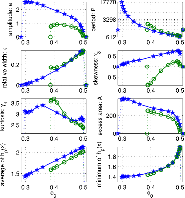
Fig.  10: (Color online) Measures characterising the regular lines as a function of $\phi_{0}$, for fixed standard $\varOmega_{0}=4.64\times 10^{-7}$ (blue line with $\star$) and for fixed $\varOmega_{0}=4.64\times 10^{-6}$ (green line with $\circ$).⁸² The other parameters are fixed at their standard values. Selected corresponding line patterns are displayed in in Fig. 11.

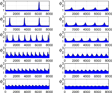
Fig.  11: (Color online) Morphology changes of the line pattern as $\phi_{0}$ is varied, corresponding to Fig. 10. Left column: For fixed standard $\varOmega_{0}=4.64\times 10^{-7}$ and, from the top to the bottom, $\phi_{0}=0.3016,0.34,0.41,0.475,0.494,0.5$, and other parameters are standard. Right column: For fixed $\varOmega_{0}=4.64\times 10^{-6}$ and, from the top to the bottom, $\phi_{0}=0.389,0.4,0.41,0.46,0.49,0.499$, and other parameters are standard.

3.3 Regular patterns in the $(\varOmega_{0},\phi_{0})$ plane

Having discussed the dynamics of the deposition process (section 3.1) and the main types of transient and long-time deposition patterns (section 3.2), we now embark on a more detailed analysis of the morphology of the regular line patterns and its dependence on the location in the parameter plane $(\varOmega_{0},\phi_{0})$. On the basis of our exploration of this parameter plane we detected regions of characteristic deposition patterns – see Fig. 9. The sub-regions marked by letters in Fig. 9 relate to the patterns under the same letters in Fig. 8 and the list of typical patterns in Sec. 3.2. The following analysis is based on a large number of long-time simulations (for details see Appendix A) in the region (h) of periodic lines, cf. Fig. 9. Excluding the initial transient, we take a sequence of $N$ regular deposition periods (lines), where $10\lessapprox N\lessapprox 100$, depending on the spatial period of the deposit and the required CPU time. We process the profiles and extract measures that characterise the individual lines and their arrangement. In particular, we obtain the amplitude $a$, spatial period $P$, relative width $\kappa=2\sigma/P$ (where $\sigma$ is the standard deviation), skewness $\gamma_{3}$, kurtosis $\gamma_{4}$, excess cross-sectional area of the lines $A$, the mean deposit height $\overline{{h_{\mathrm{p}}}}$, and the minimal height of the deposit between the lines $\tilde{h_{\mathrm{p}}}$. Definitions of all these measures are given in Appendix B. Our investigation shows that these quantities strongly depend on both the evaporation number $\varOmega_{0}$ and the concentration $\phi_{0}$. We focus on two vertical and two horizontal cuts through the parameter plane $(\varOmega_{0},\phi_{0})$ that are indicated by dashed straight lines in Fig. 9.

First, we vary the concentration $\phi_{0}$ for two evaporation numbers, $\varOmega_{0}=4.64\times 10^{-7}$ and $\varOmega_{0}=4.64\times 10^{-6}$, while the remaining system parameters are fixed at our standard values (see end of section 2). Fig. 10 presents the line characteristics for both cases and Fig. 11 shows a number of corresponding deposit profiles.

Most of the line characteristics behave qualitatively similar for the two cases. We first focus on $\varOmega_{0}=4.64\times 10^{-7}$ and then point out the differences. On increasing $\phi_{0}$ from a region where there is no deposition of periodic lines, one first encounters large amplitude almost solitary peaks that are separated by very large distances. On further increasing $\phi_{0}$, the amplitude first hardly changes and later decreases. The period rapidly decreases while the relative line width and skewness increase almost linearly with a slight drop in skewness at very high concentrations $\phi_{0}\gtrapprox 0.49$. For higher $\phi_{0}$, the deposit pattern almost turns into a constant thickness layer, with a small amplitude harmonic modulation. Finally, the amplitude goes to zero (at finite period) at the upper border of region (h). For $\varOmega_{0}=4.64\times 10^{-6}$, the evaporation is stronger and one must go to a higher $\phi_{0}$ than when $\varOmega_{0}=4.64\times 10^{-7}$, to see periodic deposition of lines. The period of the lines does not seem to diverge at this border and the amplitude of the lines is much smaller. Actually, the amplitude first increases with increasing $\phi_{0}$ and has a maximum well inside the region of regular lines before it decreases towards zero at the other border of the region. Interestingly, in contrast to the former case, the skewness changes from negative to positive values, i.e., the individual lines change their morphology from having a ‘tail’ away from the receding front to having a tail in the direction towards the front, as is always the case for $\varOmega_{0}=4.64\times 10^{-7}$. In both cases the excess area greatly decreases, the minimum height of the deposited valleys between lines greatly increases, and the period and amplitude decrease as the boundary of region (h) at higher $\phi_{0}$ is approached. The average height of the deposit linearly increases with the concentration as expected but, interestingly, the two linear dependencies for the two evaporation rates are shifted with respect to each other. This aspect is further discussed in Appendix A.2.

Fig.  12: (Color online) Measures characterising the regular lines as a function of $\varOmega_{0}$, for fixed standard $\phi_{0}=0.41$ (blue line with $\star$) and for fixed $\phi_{0}=0.31$ (green line with $\circ$).⁸² The rest of the parameters are fixed at the standard values. Selected corresponding line patterns are displayed in Fig. 13.

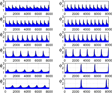
Fig.  13: (Color online) Morphology changes of the line pattern as $\varOmega_{0}$ is varied, corresponding to the results in Fig. 12. Left column: Fixed standard $\phi_{0}=0.41$ and, from the top to the bottom, $\varOmega_{0}=(0.1598,0.1667,0.3162,1,5.274,5.663)\times 10^{-6}$. Right column: Fixed $\phi_{0}=0.31$ and, from the top to the bottom, $\varOmega_{0}=(1,1.137,1.468,2.15,3.162,4.083)\times 10^{-7}$.

Second, we vary the evaporation number $\varOmega_{0}$ for two concentrations $\phi_{0}=0.41$ and $\phi_{0}=0.31$, while the remaning parameters are fixed at our standard values (see end of section 2). Fig. 12 presents the line characteristics for both cases and Fig. 13 displays a number of the corresponding deposit profiles.

We first focus on the case $\phi_{0}=0.41$ and then point out the differences found for the lower concentration value. Increasing $\varOmega_{0}$, one moves from the narrow region (d) of transient multiple lines (see Fig. 9), passes through a very narrow band of intermittent line patterns (g) followed by the region (h) in which we observe the regular line patterns. For the lowest values of $\varOmega_{0}$ in (h), the patterns have a relatively small period and a small but non-zero amplitude. The strongly anharmonic peaks are skewed to the right with their tail pointing towards the wet side. On increasing $\varOmega_{0}$ the period increases. The amplitude, however, first increases and then decreases, until at a certain threshold, the pattern ceases to be periodic and we arrive in the narrow border region (c), where only a finite number of lines are deposited. Correspondingly, the relative width of the lines decreases as one moves deep into the region of periodic lines, where the lines become more peaked. Remarkably, the skewness changes sign here, i.e. as $\varOmega_{0}$ increases the tail of the lines shifts from pointing towards the receding wet film, to pointing away.

The second cut with varied $\varOmega_{0}$ is at fixed $\phi_{0}=0.31$ and the standard values for the remaining parameters. For small $\varOmega_{0}$, the onset is similar as for the previous cut at $\phi_{0}=0.41$. However, on increasing $\varOmega_{0}$, one finds large-amplitude long-period line patterns. The period seems to diverge in a manner similar to that found when increasing $\phi_{0}$ for fixed $\varOmega_{0}=4.64\times 10^{-7}$ (see Fig. 10). Note that in Fig. 12 the average deposit thickness changes as $\varOmega_{0}$ is varied, even though the initial concentration $\phi_{0}$ is fixed. The deposited average thickness for more dilute solute concentrations can be higher than when a denser solution is used, as long as the evaporation rate is higher. This effect stems from the influence the moving evaporation front has on the concentration field in the thick liquid film. This is related to our boundary conditions and is further discussed at the end of Appendix A.2.

Note, that a change in the sign of the skewness as described above, was also observed in experiments on nanoparticle suspensions ⁸³ and can be explained as follows: For smaller values of $\varOmega_{0}$ and/or higher $\phi_{0}$, the capillary ridge is large and accommodates a large amount of solute as it recedes. When the front pins, the capillary ridge evaporates and the solute contained in the ridge is deposited in a thick tail pointing towards the receding front. When the liquid front depins, it carries much of the solute within the liquid front away with it, which results in a further drop in the deposition thickness (seen as the final shoulder of the tail). For higher values of $\varOmega_{0}$ the capillary ridge is smaller and so the tail pointing towards the receding front is smaller. On the other hand a negative skewness is typical for higher $\varOmega_{0}$ and (possibly) low $\phi_{0}$. There, one encounters smaller tails towards the receding front and also a pronounced tail away from the front. In this situation, it takes some time (during which the front travels some distance) for the solute concentration to build up at the front. During this time the front gradually slows down and deposits the solute with growing thickness until local jamming occurs. Then the front pins and starts to deposit a line. The resulting asymmetry is seen as negative skewness.

3.4 Onset of formation of periodic deposits

To further clarify how the onset of pattern formation occurs we next focus on the small band in the parameter plane $(\varOmega_{0},\phi_{0})$ that bounds the region of periodic deposits. From inspecting Fig. 9 and the line deposition descriptions outlined in the previous section, one clearly sees that the onset of the formation of periodic deposits may occur through a number of different transitions.

The most intricate transition is the one that involves the intermittent deposits shown in Fig. 8(g) and (e), and occurs in the narrow region (g) of Fig. 9. We find that this behaviour is very sensitive to computational details (which is not the case for the regular line patterns), a fact which bolsters our opinion that the intermittent line patterns represent a ‘chaotic deposition’. Taken in this context, the occurrence of periodic deposits of double lines (Fig. 8(f),(i) would be related to the periodic deposition of single lines through a period doubling bifurcation that occurs when changing the relevant control parameter. Both effects point towards the presence of chaos in the system, as they are elements of the intermittency and period-doubling route to chaos, respectively.⁸⁴ However, to investigate these effects further, simpler asymptotic models for the moving material-depositing front need to be constructed that are numerically less challenging.

fixed	$\varOmega_{0}=4.64{\cdot}10^{-7}$	$\phi_{0}=0.41$		$\varOmega_{0}=4.64{\cdot}10^{-6}$
varied	high $\phi_{0}$	low $\varOmega_{0}$	high $\varOmega_{0}$	low $\phi_{0}$	high $\phi_{0}$
$\varDelta_{\mathrm{abs}}$	0.0004	0.0359	0.0546	0.0134	0.0023
$\varDelta_{\mathrm{rel}}$	0.0018	0.0197	0.0299	0.0596	0.0102

Table 1: The measured hysteresis intervals, $\varDelta_{\mathrm{abs}}$ and $\varDelta_{\mathrm{rel}}$, are listed for the various transitions between the long-time deposition of periodic patterns and flat layers that occur along the straight lines in Fig. 9. In these intervals different deposition patterns may be obtained, depending on initial conditions. The first row indicates which parameter is held fixed whilst the second row states which parameter is varied and which border of the region of periodic deposits is being considered. The third row gives the absolute hysteresis interval $\varDelta_{\mathrm{abs}}$ in terms of the parameter that is being varied, whereas the fourth row gives the relative interval size $\varDelta_{\mathrm{rel}}=\varDelta_{\mathrm{abs}}/\varDelta$, where $\varDelta$ is the corresponding size of the entire region of periodic deposits in the $(\log_{10}\varOmega_{0},\phi_{0})$ plane ($\varDelta=1.8239$ in $\log_{10}\varOmega_{0}$ coordinate and $\varDelta=0.225$ in $\phi_{0}$ coordinate). Note that $\varDelta_{\mathrm{abs}}$ is measured in terms of the particular parameter that is being varied (either $\log_{10}\varOmega_{0}$ or $\phi_{0}$), i.e., it represents a length in the semilogarithmic phase plane Fig. 9. Note, that we do not include results for fixed $\varOmega_{0}=4.64{\times}10^{-7}$ at low $\phi_{0}$. There the line period becomes very large and long pieces of nearly flat layers occur between the lines. This results in rather expensive computations. However, our limited results indicate that there is no hysteresis in this case.

In general, it has proved to be difficult to detect the exact location of the boundary of the region of periodic line deposits. A detailed study reveals that close to the boundary different patterns may often emerge for identical parameter values, depending on the initial condition. In other words, many of the transitions are hysteretic: If one starts inside the region (h) of Fig. 9 with a simulation that gives regular lines and then moves by small parameter increments closer to the boundary one can detect at which parameter values the deposit turns into a layer of constant thickness, and in this way define a boundary of region (h). However, alternatively one may start in the region outside (h), where after some initial transient one obtains a flat deposit layer, and then slowly move towards the boundary of (h). Detecting at which parameter value the flat deposit turns into a regular line pattern, one finds that this transition occurs at a point inside the region (h), i.e. there is a small hysteretic region where both patterns may occur. Using this technique we numerically obtain the width of the hysteresis region on the cuts through the $(\varOmega_{0},\phi_{0})$ parameter plane that were discussed in section 3.3 and indicated in Fig. 9. The results for the width of the hysteresis region are listed in Table 1.

From our investigations of the transitions in the $(\varOmega_{0},\phi_{0})$ plane, we find four typical scenarios for the onset of the formation of periodic line patterns:

• At low $\phi_{0}$ and small or intermediate $\varOmega_{0}$ the spatial period of the lines diverges while the line amplitude first slowly increases and then converges to a finite value (see Fig. 10). This indicates the occurrence of an infinite period bifurcation, that could be either a SNIPER (Saddle Node Infinite PERiod) bifurcation or a homoclinic bifurcation.⁸⁴ The fact that for $\varOmega_{0}=4.64{\times}10^{-7}$ we do not see any hysteresis (see Table 1) points towards a SNIPER bifurcation, as a homoclinic bifurcation often involves some hysteresis between a stable steady or stationary state (in the present case, the deposition of a flat layer) and a stable time-periodic state (here, the deposition of line patterns). Note, however, that we are not able to come sufficiently close to the bifurcation point to test whether the typical power law relation between the period and the distance to the bifurcation point also holds here. A similar behaviour is found at high $\varOmega_{0}$ and fixed $\phi_{0}=0.31$ (Fig. 12). We discuss further at the end of this section how this finding compares to results for depinning transitions in other soft matter systems.

• For high evaporation rates $\varOmega_{0}$ and high $\phi_{0}$ the line amplitude decreases with increasing $\varOmega_{0}$ as the boundary of region (h) is approached, before suddenly jumping to zero (see Fig. 12). At the same time, the line period tends to a finite value. Outside region (h), the pattern ceases to be periodic and the simulations show an initial transient deposition of a finite number of lines, followed by a flat layer. Since the hysteresis here is rather large (see Table 1), we conclude that the transition most likely corresponds to a subcritical Hopf bifurcation.

• For low $\varOmega_{0}$ and all but the very small values of $\phi_{0}$, as the boundary is approached the line amplitude first decreases (with increasing rate) with decreasing $\varOmega_{0}$, before suddenly jumping to zero (see Fig. 12). At the same time, the line period tends to a finite value. Just outside this boundary to region (h) the simulations exhibit a transient deposition of a finite number of lines, followed by a flat layer. Since there is some hysteresis (see Table 1), at first sight the transition seems to correspond to a subcritical Hopf bifurcation, and therefore seems to be rather similar to the case described in the previous point (ii). However, at intermediate $\phi_{0}$, close to the boundary of (but within) region (h) one sees signs of a period doubling and there is also the band of intermittent patterns of type (g) just outside of region (h) [cf. Fig. 13 (left column, first panel) and Fig. 8(g) and (e), respectively]. This indicates that the transition might involve several complex eigenvalues and be related to the intermittency and period-doubling route to chaos.⁸⁴ Whatever is happening at the boundary, it is certainly more complex than case (ii).

• The last case we mention is a hypothetical transition scenario that we did not see but that we believe is likely to occur. Our study is based on a model that can be computationally expensive, especially for values of $(\varOmega_{0},\phi_{0})$ that are close to the onset of the deposition of periodic lines. Table 1 shows that the width of the hysteresis region $\varDelta_{\mathrm{abs}}$ varies along the boundary. In particular, at large concentrations $\varDelta_{\mathrm{abs}}$ becomes very small. We believe it is likely that there may exist a small interval along the boundary where there is no hysteresis, i.e., $\varDelta_{\mathrm{abs}}=0$, and the line amplitude gradually decreases to zero while the line period approaches some non-zero value, and the deposition pattern becomes a small amplitude harmonic modulation. Such a transition would correspond to a supercritical Hopf bifurcation.

Note, that the present study only considers one-dimensional deposition patterns. Two dimensional deposition patterns are beyond our scope. We expect the full two-dimensional behaviour to be very rich. In particular, at small evaporation rates one should expect the evaporative dewetting front to be transversally unstable, even in the situation without solute.⁷⁵ We expect this to also occur in the case with solute, close to the transition discussed in points (i) and (iii). This argument is bolstered by the observation that the particular transition described in (i) involves deposits that are nearly homoclinic in space. There exist generic results ⁸⁵ that show that patterns near homoclinic solutions are prone to instabilities.

Before we move on to discuss in the next section the influence of system control parameters besides the solute concentration $\phi_{0}$ and the evaporation number $\varOmega_{0}$, we make a few comments to put our findings into a wider context. It is important to understand that the observed transitions from stationary front motion to the deposition of lines may be seen as depinning transitions in the frame moving with the mean front speed: When a front of constant speed deposits a flat layer, in the comoving frame the concentration profile is steady. Then, one may say that the concentration profile is pinned to the moving front as it does not move relative to it. However, at the transition to depositing a periodic pattern, the concentration profile starts to stay behind the moving front, and one may say it depins from the front. Note, however, that after depinning, the concentration profile does not move relative to the front as a whole. Instead, only a part of it (the jammed part) starts to move relative to the front, resulting in the deposition of a line. This process then repeats periodically.

From this observation it becomes clear why the transition scenarios (i) to (iv) described above are analogous to similar scenarios found in studies of depinning in other driven soft matter systems. To illustrate how universal such transitions are, we mention three systems: First, drops of simple nonvolatile liquids that sit on heterogeneous substrates and depin from the heterogeneities under the influence of external driving forces. Depending on the particular setting and parameter regime, one may observe SNIPER, homoclinic and super- or subcritical Hopf bifurcations.^{86, 87, 88} There, however, the entire depinning drop or ridge slides along the heterogeneous substrate in a periodic manner. A second system consists of clusters of interacting colloidal particles that shuttle under the influence of external forces through a heterogeneous nanopore.^{89, 90} Under weak dc driving, the peak in the particle density distribution is pinned by the heterogeneities of the pores. However, depending on driving force and the attraction between the colloids, depinning transitions via Hopf and homoclinic bifurcations occur resulting in time periodic fluxes. The third system is much closer related to the one studied here, as it also concerns patterns that are produced at a three-phase contact line: If a Langmuir–Blodgett surfactant monolayer is transferred from a bath onto a solid substrate, one may observe stripe patterns in the deposit resulting from substrate-mediated condensation.^{50, 51, 52} Time simulations of a dynamical model for this system show the occurrence of patterns of stripes parallel to the contact line (and other patterns too).⁶³ In a reduced model the depinning transitions from a steady (pinned) concentration profile to the time periodic (depinned) state may occur via a homoclinic bifurcation or a subcritical Hopf bifurcation.⁹¹

The comparison with these different soft matter systems that show depinning, corroborates the picture we have given above in points (i) to (iv). However, a systematic analysis of the various transitions related to the onset of the deposition of line patterns in the present system requires a simplified model to be developed.

In the following sections we briefly describe how varying other physical aspects of the system influence the behaviour of the system. In Sec. 3.5 we examine the effect of varying the diffusivity of the solute in the solvent. In Sec. 3.6 we discuss the influence of varying the wettability and also of varying the chemical potential of the solvent in the ambient vapour. In Sec. 3.7 we discuss effects of solvent rheology.

3.5 Influence of diffusion

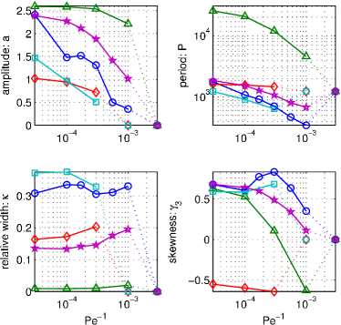
Fig.  14: (Color online) Measures characterising the regular line patterns as a function of $\mathrm{Pe}^{-1}$ for fixed parameters:⁸² $\star$ (purple line), the standard parameter values; $\circ$ (blue line), $\varOmega_{0}=1.667\times 10^{-7},\phi_{0}=0.41$; $\scriptstyle\triangle$ (green line), $\varOmega_{0}=4.64\times 10^{-7},\phi_{0}=0.3016$; $\scriptstyle\diamondsuit$ (red line), $\varOmega_{0}=5.663\times 10^{-6},\phi_{0}=0.41$; and $\scriptstyle\square$ (light blue line), $\varOmega_{0}=4.64\times 10^{-7},\phi_{0}=0.498$. The purple line corresponds to states in the central part of the region (h) on Fig. 9, whereas the other lines correspond to points close to its boundary. Selected corresponding line patterns are shown in Figs. 15 and 16. Note, that for $\scriptstyle\triangle$ (green) the period $P$ monotonically increases to very large values with decreasing $\mathrm{Pe}^{-1}$ (up to $P\approx 30000$ at $\mathrm{Pe}^{-1}=0$).

Fig.  15: (Color online) Morphology changes of the line pattern as $\mathrm{Pe}^{-1}$ is varied, corresponding to Fig. 14. The left column shows profiles corresponding to the blue line with $\circ$ symbols and the right column to the purple line with $\star$ symbols in Fig. 14. From top to bottom, the panels in both columns correspond to $\mathrm{Pe}^{-1}=3\times 10^{-5},10^{-4},1.7\times 10^{-4},3\times 10^{-4},5.6\times 10^{-4}$ and 0.001.

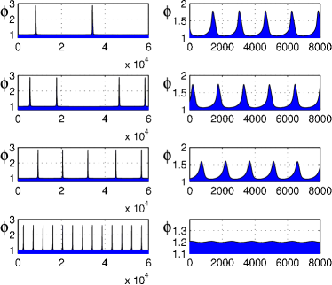
Fig.  16: (Color online) Morphology changes of the line pattern as $\mathrm{Pe}^{-1}$ is varied, corresponding to Fig. 14. The left column shows profiles corresponding to the green line with $\scriptstyle\triangle$ symbols and the right column to the red line with $\scriptstyle\diamondsuit$ symbols in Fig. 14. From top to bottom, the panels in both columns correspond to $\mathrm{Pe}^{-1}=3\times 10^{-5},10^{-4},3\times 10^{-4}$ and 0.001.

The influence of diffusion is quantified in our model by the inverse Péclet number $\mathrm{Pe}^{-1}$. Up to this point we have discussed the basic mechanism as being based on a subtle balance of convective and evaporative motion. In the results presented so far, the solute diffusivity was low and contributed little to the overall transport.

Fig. 14 presents results for several measures which characterise the periodic line patterns, as a function of the inverse Péclet number $\mathrm{Pe}^{-1}$, which is a ratio of the time scales for convection and diffusion. Results are shown for five sets of values of the parameters $(\varOmega_{0},\phi_{0})$, corresponding to locations within the region of periodic lines [region (h) in Fig. 9]: symbols $\star$ indicate our standard values of $(\varOmega_{0},\phi_{0})$ and the other sets correspond to locations close to the boundary of region (h). Examples of the corresponding line patterns are displayed in Figs. 15 and 16. All the other parameters, $\chi$, $M$, and $\nu$ are equal to the standard values (see the end of Section 2).

Around and below the standard value of $\mathrm{Pe}^{-1}=0.0003$, the deposition pattern is almost independent of the value of $\mathrm{Pe}^{-1}$. Decreasing $\mathrm{Pe}^{-1}$ to zero has almost no effect on the size of region (h), and the only effect is that the deposit patterns becomes slightly sharper. However, on increasing $\mathrm{Pe}^{-1}$ above $0.0003$, the size of the region (h) (Fig. 9) starts to shrink considerably, until it vanishes entirely as the effects of solute diffusion increase (roughly, when $\mathrm{Pe}^{-1}>0.003$). The shape of the lines changes monotonically and they become more sinusoidal in shape: the amplitude, period and skewness all become smaller with increasing $\mathrm{Pe}^{-1}$, while the relative width, $\kappa=2\sigma/P$ increases (see Fig. 14). We remind the reader that highly peaked or separated lines have small $\kappa$ values, whereas a deposit profile that resembles a harmonic wave has a large $\kappa$ value. When the diffusive mobility of the solute is large the effect of diffusion counteracts the solute build up due to evaporation. The transition between the deposition of periodic lines and a flat layer occurs in between $\mathrm{Pe}^{-1}=0.001$ and $\mathrm{Pe}^{-1}=0.003$ for the standard values of $(\varOmega_{0},\phi_{0})$ and at somewhat smaller $\mathrm{Pe}^{-1}$ for parameter values close to the boundary of region (h), as the region itself is shrinking. Such a large diffusivity is unlikely for large nanoparticles in suspension but might occur for very small particles or for small molecules in solution. Since the line amplitude approaches zero at this transition point, whilst the period remains finite and the line profiles become nearly harmonic, we suspect that this transition corresponds to a Hopf bifurcation (cf. section 3.4) but we did not study this transition in as much detail as the transitions discussed in Sec. 3.4.

In the lower right panel of Fig. 14 we display results obtained for the skewness, $\gamma_{3}$. As $\mathrm{Pe}^{-1}$ is increased, the curves marked by symbols $\circ$ and $\scriptstyle\square$ show at first an increase of $\gamma_{3}$ before it decreases again just before the pattern vanishes. The reason for this non-monotonic behaviour can be seen in the left column of Fig. 15 that displays deposit profiles which correspond to the $\circ$ curve in Fig. 14. There, going from the first to the fourth panel from the top we see new secondary lines emerge out of the tail of the primary lines, i.e., decreasing the effects of diffusion, leads to a period doubling. The period doubling is not visible in the dependence of the period on $\mathrm{Pe}^{-1}$ (see Fig. 14) because around these parameter values the pattern is not very regular and the secondary lines appear through a smooth transition. These irregular patterns seem to be analogous to the intermittent patterns [Fig. 8(g)] or the depression–line patterns [Fig. 8(j)] but here these intermediate patterns appear in a somewhat wider band of parameter values close to the border of region (h) in the phase plane shown on Fig. 9. The period of these irregular patterns $P\approx P_{\mathrm{shift}}/2$, which indicates that the shift length (see Appendix A) interacts with the period of the pattern. In general, all such irregular patterns appear only close to the boundary of region (h) (Fig. 9) of periodic lines, where $\varOmega_{0}$ is small and $\phi_{0}$ is moderate to high. In other words, where patterns have large positive $\gamma_{3}$ (heavy right tail), we observe the ‘chaotic deposition’ described in Sec. 3.4, and we expect transversal instability effects. In Appendix A.3 we discuss how robust the results we obtain are, in relation to the numerical methods we use to solve our model equations. The profiles in Figs. 15 and 16 also show that as the value of $\mathrm{Pe}^{-1}$ is increased, the parameter regions where lines of large positive skewness (long tail towards front) are found (smaller $\varOmega_{0}$ and moderate and high $\phi_{0}$) become replaced by lines that are nearly symmetric (small skewness) or point the tail away from the front (negative skewness). In addition, the period of the lines decreases.

Finally, we mention the importance of diffusion in experiments and applications of such evaporation driven self-organisation processes. The relative importance of diffusion depends on both the mobility of the solute and the thickness of the solution layer. For instance, for very thin films ^{19, 13} one sees from Eqs. (3) and (5), that the diffusive mobility $Q_{\mathrm{d}}\propto h$ dominates the convective mobility $Q_{\mathrm{c}}\propto h^{3}$; see also the discussion by Vancea et al. ⁹², where the dynamics in ultrathin postcursor films left behind mesoscopic dewetting fronts of nanoparticle suspensions ¹³ is modelled by either kinetic Monte Carlo models ^{93, 92, 94} or dynamical density functional theory ^{95, 96} that only incorporate diffusive transport because in this situation diffusion is the dominant process. The present thin film model captures the competition of convective and diffusive transport relevant for larger film thicknesses where the key influence is the mobility of the solute itself. Xu et al. ²⁵ found that as the size of nanoparticles is decreased, one obtains spoke-like structures and irregular patterns instead of the regular rings seen for larger nanoparticles. This indicates that an increase of the influence of diffusion brings the system closer to the border of the region of periodic line deposition, where patterns become irregular and unstable in accordance with our present findings.

In summary, a low value for the solute diffusivity means diffusion does not influence the deposition patterns and diffusion may actually be neglected in the model. However, fast diffusion is able to counteract evaporation and effectively suppresses the occurrence of deposition patterns.

3.6 Influence of wettability and chemical potential

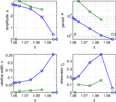
Fig.  17: (Color online) Measures characterising the regular lines as a function of $\chi$.⁸² The blue lines with $\circ$ symbols have fixed $\varOmega_{0}=7\times 10^{-7}$, and the standard concentration $\phi_{0}=0.41$, whilst the green lines with $\scriptstyle\square$ symbols have the (standard) evaporation rate $\varOmega_{0}=4.64\times 10^{-7}$ and concentration $\phi_{0}=0.31$. All other parameter values are the standard ones, defined at the end of Sec. 2. The blue lines corresponds to configurations in the central part of the region (h) on Fig. 9. Selected line patterns corresponding to these are shown in Fig. 18. Note that the period $P$ seems to decrease exponentially with increasing $\chi$ but we also note that for $\chi$ smaller than the standard value, we observe stable double lines.

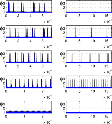
Fig.  18: (Color online) Morphology changes as $\chi$ is varied, corresponding to the results in Fig. 17. Left column: the profiles correspond to the blue lines with $\circ$ symbols in Fig. 17; from top to bottom the results are for $\chi=1.06,1.062,1.065,1.075$ and $1.095$. Right column: corresponding to the green lines with $\scriptstyle\square$ symbols in Fig. 17; from top to bottom the results are for $\chi=1.062,1.065,1.075,1.085$ and $1.095$. The other parameters have the standard values.

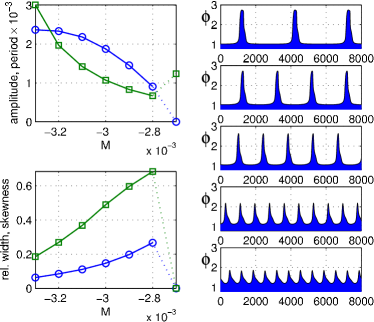
Fig.  19: (Color online) Left column: Measures characterising the regular line pattern as $M$ is varied.⁸² The upper panel shows both the amplitude (blue line with $\circ$ symbols) and the period (green line with $\scriptstyle\square$). The Lower panel shows the relative width (blue line with $\circ$) and skewness (green line with $\scriptstyle\square$). All the parameters except $M$ have the standard values as defined at the end of Sec. 2. Right column: Corresponding profiles for $M=-(3.3,3.2,3.1,2.9,2.8)\times 10^{-3}$, from top to bottom.

After having discussed the influence of solute diffusion in the previous section, here we briefly consider the influence of wettability and the chemical potential of the solvent vapour. We start with the influence of the wettability that is quantified in our model by the parameter $\chi$, contained in the polar contribution to the disjoining pressure $\varPi=1/h^{3}-\exp(-\chi h)$. The influence of changes in $\chi$ on $\varPi$ can be appreciated by inspecting Fig. 3. A decrease [increase] from our standard value $\chi=1.085$ results (at fixed chemical potential $M$) in a decrease [increase] of the precursor film thickness and of the thickness of the bulk film; an increase [decrease] of the thickness where the front profile has its inflection point; a decrease [increase] of the wetting energy at the precursor film height, and in consequence an increase [decrease] of the slope at the inflection point, that is our measure of a ‘nonequilibrium contact angle’. It also leads to larger [smaller] energy difference between the two stable heights, $h_{1}$ and $h_{2}$, so the evaporation will be stronger [weaker].

Corresponding results for the deposition patterns are displayed in Fig. 17 (line characteristics) and Fig. 18 (selected deposition profiles). The line amplitude and period decrease monotonically with increasing $\chi$, while the skewness first increases and then drops in value. The period, amplitude and relative width behave in a similar manner as when increasing $\phi_{0}$, see Sec. 3.3. This indicates that the transition towards a flat deposit at large $\chi$ is most likely via a Hopf bifurcation, i.e. via scenario (ii) or (iv) discussed in Section 3.4. On decreasing $\chi$, we find that the lines become more anharmonic and sharper and after a period doubling become deposited in pairs. A further decrease results in groups of multiple lines and in general to the deposition of a more irregular pattern, i.e. the transition towards a flat deposit at small $\chi$ is most likely via scenario (iii) introduced in Section 3.4. Some corresponding profiles are displayed in the left hand column of Fig. 18.

The main features of an evaporative dewetting front are influenced not only by $\chi$, but also by the dimensionless chemical potential $M$ (cf. Fig. 3). A decrease in $M$ at fixed $\chi$ results in a decrease of the precursor film thickness and also of the upper film thickness; an increase of the thickness where the front profile has its inflection point; a small increase of the wetting energy at precursor film height but also in an increase of the energy difference between the two stable heights, $h_{1}$ and $h_{2}$; and, as a consequence an increase of the contact angle. A further decrease in $M$ leads to faster evaporation in the front region, i.e., a larger front velocity, and so the capillary ridge decreases and the ’nonequilibrium contact angle’ decreases. Many of these features can already be seen in the case without solute.⁷⁵

Results obtained for varying $M$ are presented in Fig. 19. A decrease in $M$, i.e. increase in $|M|$, results in an increase of the line amplitude and period. We do not consider $M<-0.0033$ as then no second stable film height exists, a case not covered by our numerical set-up. Increasing $M$, the line amplitude decreases towards zero, the period approaches a constant value and the relative width and skewness of the lines both increase. This is similar to the case of increasing $\chi$ (compare the two columns of Fig. 17). We see this as an indication of a Hopf bifurcation as the most likely transition mechanism, i.e. scenario (ii) or (iv) of Section 3.4. If this is correct, the skewness should decrease strongly over a small range of values of $M$. Note finally, that it is difficult to separate the influences of the parameters $\chi$ and $M$ as they both influence the stable film heights, the contact angle, and whether a capillary ridge exists or not.

3.7 Influence of solution rheology

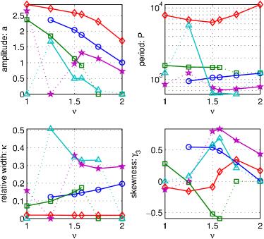
Fig.  20: (Color online) Measures characterising the line pattern as a function of the viscosity exponent $\nu$.⁸² The blue curve with $\circ$ symbols is for fixed standard $\varOmega_{0}=4.64\times 10^{-7}$ and standard $\phi_{0}=0.41$; The green curve with $\scriptstyle\square$ is for $\varOmega_{0}=4.64\times 10^{-6}$ and standard $\phi_{0}$; The red curve with $\scriptstyle\diamondsuit$ is for the standard value of $\varOmega_{0}$ and for $\phi_{0}=0.31$; The light blue line with $\scriptstyle\triangle$ is for the standard value of $\varOmega_{0}$ and for $\phi_{0}=0.498$; The purple line with $\star$ is for $\varOmega_{0}=1.667\times 10^{-7}$ and standard $\phi_{0}$. All the other parameter values are standard, as defined at the end of Sec. 2. The blue line corresponds to configurations in the central part of the region (h) on Fig. 9 whereas the other lines correspond to points close to its boundary. The corresponding line patterns are shown in Figs. 21 and 22.

Fig.  21: (Color online) Morphology changes for various values of the exponent $\nu$, corresponding to Fig. 20. The left column corresponds to the blue lines with $\circ$ symbols and the right column to the red lines with $\scriptstyle\diamondsuit$ in Fig. 20. From top to bottom panels in each column correspond to $\nu=1,1.25,1.5,1.575,1.75$ and $2$.

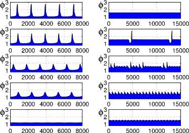
Fig.  22: (Color online) Morphology changes for various values of the exponent $\nu$, corresponding to Fig. 20. The left column corresponds to the green line with $\scriptstyle\square$ symbols and the right column to the light blue line with $\scriptstyle\triangle$ in Fig. 20. From top to bottom panels in each column correspond to $\nu=1,1.25,1.5,1.575$ and $1.75$.

In this final results section we discuss the influence of solution rheology – i.e. we present results for varying the exponent $\nu$ in the Krieger–Dougherty law (16). In the thin film literature the value $\nu=2$ is often used,^{68, 59} and our standard configuration employs the value $\nu=1.575$ corresponding to spherical colloidal particles as discussed above following Eq. (7). However, some authors suggest that for some systems, much lower values are required, in particular, in the context of jamming transitions for attractive colloidal particles. There, values as low as $\nu=0.13$ are mentioned.⁶⁹

Here we consider moderate variations in the interval $1\leq\nu\leq 2$, and investigate how the deposition patterns change for five selected points in the parameter plane $(\varOmega_{0},\phi_{0})$. Three of the configurations correspond to the crossing points of the four straight dashed lines in Fig. 9 that lie within the region (h) of periodic lines [one is the standard case described at the end of Sec. 2 and the other two lie close to the boundary of region (h)]. The other two selected points also lie close to the boundary of the region (h). Results for measures characterising the deposition patterns are displayed in Fig. 20 and selected corresponding deposition profiles are displayed in Figs. 21 and 22.

First, we consider the case of the standard set of parameter values, that is in the central part of the region (h) in Fig. 9. The measures are shown with the symbols $\circ$ (blue curve) in Fig. 20 and selected corresponding profiles are displayed in the left column of Fig. 21. As $\nu$ decreases from the value $\nu=2$, the amplitude of the deposition lines increases, the relative width decreases and the skewness departs from zero indicating that the lines become more peaked and anharmonic at lower $\nu$. Note that simulations tend to be more computationally demanding at lower $\nu$ and e.g., the point at $\nu=1.0$ has a larger error, because effects of the initial transient are still present in the analysed data.

The other selected points, located close to the boundary of region (h) in Fig. 9 behave somewhat similarly, but with some differences. The symbols $\scriptstyle\diamondsuit$ (red line) in Fig. 20 correspond to lines with a large amplitude and a long period; a selection of profiles for this case are displayed in the right column of Fig. 21. Interestingly, the period changes nonmonotonically, while the skewness decreases as $\nu$ is decreased. Profiles that correspond to the symbols $\scriptstyle\square$ (green line) in Fig. 20 are displayed in the left column of Fig. 22. The lines have negative skewness and vary with $\nu$ in a manner similar to the results for the standard set of parameter values. The symbols $\scriptstyle\triangle$ (light blue line) and $\star$ (purple line) correspond to the points close to the boundary of region (h) where period doubling transitions are observed and results become quite sensitive to the details of the numerical solution method. The computations are very sensitive for decreased $\nu$ values for the case when $\phi_{0}=0.498$, with standard $\varOmega_{0}$, which correspond to the symbols $\scriptstyle\triangle$ (light blue line) in Fig. 20, with corresponding profiles displayed in the right column of Fig. 22. There we see patterns that switch between a depression–line pair and a flat layer, and irregular intermittent patterns.

In general, the deposition of regular lines is robust with respect to a change in $\nu$ and we observe them over a broad interval of parameter values. This is to be expected from the experimental results, where periodic lines were seen for various (non)spherical nanoparticles,²⁵ colloids ⁵ and polymeric solutes.³² The general trend is for the regular line patterns to become more sharply pronounced as the value of $\nu$ becomes smaller, i.e., the line amplitude increases and their relative width decreases.

We do not study in detail the onset of periodic deposits when varying $\nu$. For very small values of $\nu$ the simulations are computationally too demanding, since the lines are more sharply peaked. For some configurations close to the boundary of region (h) in Fig. 9, we observe irregular deposits and a transition to a flat deposit indicating that region (h) may shrink as $\nu$ is decreased – cf. Fig. 22. As the value of $\nu$ is increased, the line amplitude decreases, and we expect that for values of $\nu$ larger than 2, the region of periodic deposits will also vanish.

4 Discussion and conclusion

We have presented a thin film model for the close-to-equilibrium self-organised deposition of material onto a smooth flat solid surface from a receding three-phase contact line of a polymer solution or nanoparticle suspension. The model consists of a pair of highly non-linear coupled long-wave evolution equations for the film thickness $h$ and the effective solute layer height ${h_{\mathrm{p}}}=h\phi$, where $\phi$ is the height-averaged scaled solute concentration. The evolution of the film is driven by a number of terms in the equations which describe several physical effects, including: (i) capillarity through a Laplace (or curvature) pressure, (ii) wettability through a Derjaguin (or disjoining) pressure, (iii) evaporation due to a difference in the local solvent chemical potential and that of the vapour, and (iv) forces due to gradients in the solute concentration. The transport processes that are involved in the dynamics correspond to convective and diffusive transport (both give a conserved dynamics), and evaporation (a non-conserved dynamics). An important ingredient in the model is the rheological property of the solution/suspension, that leads to an arrest of the convective motion at some critical solute concentration, e.g., at random close packing, for a suspension of spheres that have no net attractive forces between them and only interact via excluded volume repulsive interactions. To model these effects, we have employed the Krieger–Dougherty power law (6) for the viscosity, but we expect similar behaviour to occur for other such laws. The model we use is related to some other models used in the literature (e.g.,^{68, 59}, as explained in Section 2).

Numerically solving our model equations, we have investigated the deposition of regular and irregular line patterns that has been observed in numerous experiments utilising a wide range of materials and experimental set-ups. Assuming the front profiles only vary in one spatial direction, we have found that regular line patterns are formed over an extended region of the parameter space. Other one-dimensional patterns that we have encountered, include the transient deposition of a single or a finite number of lines, periodic arrays of double lines, a periodic switching between depression–line pairs and a flat layer, and irregular intermittent line patterns.

We believe that the model explains one of the basic mechanisms for the formation of regular line patterns. They result from a self-organised cycle of deposition-caused pinning-depinning events that is experimentally often described as a ‘stick-slip’ motion.^{30, 22, 26} The stick-slip motion is caused by the highly nonlinear rheology: Evaporation leads to a rapid increase of the solute concentration in the contact line region resulting in a strong increase of the viscosity. This in turn eventually leads to arrest of the convective motion of the receding front. However, the front is not entirely stuck, it still moves due to evaporation, albeit at a much slower speed. During this phase more material is deposited resulting in a line deposit. After a sufficient amount of material is deposited, the concentration in the contact line region decreases, the front depins from the line deposit, and starts moving with much greater speed. This appears to be a stick-slip motion. Thus, the self-organisation of the patterned deposit results from a subtle interplay of all three of the transport processes (convection, diffusion and evaporation) and the stick-slip motion results from the large difference in the timescales of convective and evaporative dewetting.

After establishing this basic mechanism, we have performed a detailed study to investigate the influence of solute concentration, evaporation rate, diffusion, wettability, chemical potential, and solution rheology on the patterns that are formed. In general, line patterns emerge at intermediate values of both the evaporation rate and the solute concentration, indicating that both are important quantities in the deposition. Furthermore, line patterns are suppressed when the solute diffusivity is sufficiently high, because when this occurs, the moving front is not able to collect the solute. In the opposite limit, when solute diffusion is set to zero, we find that this does not significantly affect the line patterns. In this paper, we have probed the influence of wettability solely through the parameter $\chi$ in the short-range part of the Derjaguin pressure. Our results indicate that an increase in the wettability may lead to a suppression of the patterns. Note, however, that our investigations of this aspect are not exhaustive. We have not fully studied this aspect here, because our present numerical set-up does not allow for the study of a completely wetting solution. Such a study will be pursued in the future, employing a modified set-up for the case of an active geometry. The influence of the solute on the system rheology is quite notable but not easy to categorise: decreasing the exponent $\nu$ in the power law relation between the viscosity (and diffusivity) and the solute concentration, increases the amplitude of the lines for all the values of the other parameters that we have tested. However, the influence on the period of the line pattern depends on the other parameters: it can increase, decrease or even behave in a non-monotonic manner with decreasing $\nu$.

In general, these findings are in agreement with experimental results.^{97, 25, 98, 26, 99} However, to our knowledge, no experimental study has systematically mapped out the regions where the various line patterns exist (analogue to our Fig. 9), or presented a detailed (quantitative) analysis of how the line pattern characteristics depend on the system control parameters. Therefore, before we make a comparison of the typical dependencies found in the experiments and our model, we first discuss the typical length and time scales in the deposition process.

The scales we have used [cf. Eq. (11)] for the time, $x$-coordinate, and film thickness are $\tau=3\eta_{0}\gamma/\delta|\tilde{S}^{P}|^{2}$, $\alpha=(\delta\gamma/|\tilde{S}^{P}|)^{1/2}$, and $\delta=(A/6\pi|\tilde{S}^{P}|)^{1/3}$, respectively. For our standard parameter values (see Sec. 2), we find $\tau=2.3\times 10^{-8}$s, $\alpha=2.9$nm, and $\delta=0.5$nm,⁷⁵ i.e., the line pattern in Fig. 5 has a period of $\lambda\approx 3\mu$m and the mean deposition velocity is $v\approx 1\mu$m/s. For Fig. 6 we have $\lambda\approx 3\mu$m and $v\approx 0.1\mu$m/s, whereas the periods of the patterns displayed in Fig. 10 range from about $1.7\mu$m to about $52\mu$m. These values are similar to those of the experiments by Xu et al. ²⁵. Their Fig. 1 shows line patterns with $3$–$5\mu$m periods. Fig. 2 of Xu et al. ²² gives line periods between $4$ and $20\mu$m, a range similar to results by Hong et al. ³⁹. Some characteristics that we find are rather similar to experimental findings by Bodiguel et al. ⁹⁸: The contact line velocity is similar to the $0.8\mu$m/s imposed in their Fig. 1; the spatial periodicity of the pattern in their Fig. 2 is $210\mu$m and the contact line speed is $6.2\mu$m/s; In general, their typical imposed velocities are $1$–$10\mu$m/s.

It is hard to compare with experimental results in the literature how pattern properties typically depend on the control parameters, as most works do nearly not discuss these. Some authors discuss dependencies that we are not able to measure in our simulations such as, e.g., the pinning force.²⁶ A decrease in the ring spacing with decreasing distance from the probe center is sometimes described in studies of evaporative dewetting with the meniscus technique (see Figs. 1 and 3 of Kwon et al. ⁹⁹, Figs. 2 and 3 of Lin and Granick ⁹⁷, Hong et al. ²³), and Fig. 2 of Xu et al. ²². In all mentioned cases this may be interpreted as observing a decrease in the period with increasing solute concentration and/or decreasing evaporation rate. Both of these possibilities are in accord with our results in Figs. 10 and 12, respectively. However, a decrease in the period with decreasing concentration is found by Xu et al. ²⁵, a result also reported by Xu et al. ²² when comparing evaporating polymer solutions of different initial concentrations. Adachi et al. ⁵ reports a non-monotonic dependence of the line density on the initial solute concentration. Decreasing the concentration leads to the line density slowly increasing before abruptly decreasing at the edge of the patterning region. This is not unlike our findings – see Fig. 10. A quantitative comparison is difficult, as they report observing about 1–8 rings produced with a small evaporating droplet. Related problems obstruct a detailed comparison with many of the experiments performed with circular drops, which have radial geometries, that always imply a drift in several system parameters in the radial direction. The planar geometry used by Bodiguel et al. ⁹⁸, Bodiguel et al. ²⁶ allows for a more natural comparison. However, there detailed results are given for the dependence of the pinning force on experimental parameters whereas no such results are given for the period of the line patterns. What is remarkable, is the agreement for the morphology of individual lines: Bodiguel et al. ⁹⁸ shows a rather asymmetric line profile with a negative skewness, i.e., the long tail points away from the receding contact line, similar to the profiles displayed in last two panels of the left column of our Fig. 13. Such agreement also exists with results for some unpublished experiments with nanoparticle suspensions ⁸³ where line profiles having a negative skewness and also a positive skewness were found, depending on the solvent that was used, i.e., the long tail can point either away or towards the receding contact line, respectively, similar to the transition we see that is illustrated in Figs. 12 and 13.

Within the limits of our numerical approach, particular care was taken in the analysis of the onset of the formation of lines when changing the various system control parameters. We have observed three main types of transition at the border of the region of periodic lines: (i) the line period diverges while the line amplitude converges to a finite value, (ii) the line period doubles, followed by a region of intermittent patterns, (iii) the period approaches a finite value while the amplitude first decreases before suddenly jumping to zero. We have also proposed a hypothetical fourth scenario – (iv) a case where the line period approaches a finite value while the line amplitude approaches zero. To relate these findings to dynamical systems or bifurcation theory, it is helpful to consider a stationary moving front that deposits a homogeneous layer as a steady state in a comoving reference frame. At the onset of the line formation this steady state becomes unstable and gives way to a time-periodic solution (in the frame that moves with the mean speed of the front). In this context, the above mentioned transitions can be identified as (i) an infinite period bifurcation (either homoclinic or Saddle-Node Infinite PERiod (SNIPER)), (iii) a subcritical Hopf, and (iv) a supercritical Hopf bifurcation, respectively. Case (ii) is more complicated and resembles the period doubling and intermittency route to chaos when approaching the transition from the side of the periodic deposits. Approaching the transition from the side of the flat deposit, one finds that the length of the transient seems to diverge, which is similar to the transition from an excitable medium to one that exhibits sustained oscillations. In particular, the homoclinic bifurcation and the subcritical Hopf bifurcation have recently been identified to be responsible for the transition to stripe-like deposition patterns in the Langmuir–Blodgett transfer of a surfactant layer onto a moving plate, where patterning is due to substrate-mediated condensation of the surfactant.^{63, 91}

To put these transitions in a wider context, we would like to point out that the onset of stripe formation can also be seen as a depinning transition: When a homogeneous layer is deposited from a stationary moving front, the concentration profile of the solute is pinned to this front. However, this is not the case when lines are deposited. In this case, the lines are depinned from the average-velocity comoving frame – i.e. they stay behind the moving front. Note however that many details of the present transition are unlike the depinning via a homoclinic or SNIPER bifurcation described by Beltrame et al. ⁸⁸ who study how a drop depins from a substrate heterogeneity under the influence of an external driving force, leading to the entire drop sliding along the substrate. Here, after depinning, the concentration profile at the moving front does not move in its entirety away from the front. Instead, only a part of it (a line) starts to move - a process that is then repeated periodically. Note that for other parameter values for the driven drop system, the depinning transition may also be due to a Hopf or a SNIPER bifurcation.⁸⁶ The present system appears to be more complicated, as the three main types of transition can be altered by interactions with period-doubling bifurcations and/or intermittent behaviour. We believe it is necessary for reduced models to be developed in order to investigate these issues in detail. Although our understanding of the onset of the patterning is still not complete, we hope that this aspect of our investigation may prove useful in the classification of future experimental results for the onset of the formation of deposition patterns.

In the present work we have limited our attention to a one-dimensional geometry, i.e., we have studied deposition from a receding straight front with an imposed transversal stability of the front. A fully two-dimensional treatment is worth pursuing (but computationally not feasible using the numerical approach taken here – see appendix A) and highly relevant, since it is well known that receding contact lines may be transversally unstable, in particular, if the receding liquid is a suspension or solution with a volatile solvent.^{28, 12, 100, 25, 13} Experimental results on line deposition indicate that such transversal instabilities are likely to occur on the left and/or upper border of the region of line patterns in the phase diagram we have presented in Fig. 9. In the experiments by Hong et al. ²³ and Xu et al. ²⁵ transversal instabilities occur at very small velocities of the receding contact line, i.e., when the evaporation is slow and/or the solute concentration is high. In our model, we have observed that under these conditions the deposition process shows period doubling and results become very sensitive to numerical details, which suggests the system may be transversally unstable, in agreement with these experiments. In the system studied by ²¹, different types of transversal instabilities occur at low and high solute concentrations. However, this system represents an example of an active geometry where the sliding velocity of an upper plate controls the patterns that are formed. Karthaus et al. ²⁸ states that a Plateau–Rayleigh instability of the rim at the moving front is responsible for the fingering instability, an observation which is in line with arguments made for receding fronts of non-volatile ¹⁰¹ and volatile ⁷⁵ pure liquids. However, the name “Plateau–Rayleigh instability” might be misleading in the case of a moving front of a solution or suspension since (i) the motion of the liquid rim itself may change the character of the instability,¹⁰² (ii) partial wettability may trigger an instability of a receding front,¹⁰² and, most importantly, (iii) since the solute concentration may change along the front, new classes of instabilities are possible, which are related to mobility contrasts and local phase separation ⁹⁶ or solutal Marangoni effects. These possibilities warrant future studies employing either geometries that allow for a more efficient numerical approach and/or the development of reduced models in a similar spirit to the model for Langmuir–Blodgett transfer of a surfactant layer developed by Köpf et al. ⁹¹. A thin film model for this process predicts a transition from stripes that are perpendicular to the receding front, to parallel, as the transfer velocity is increased.⁶³ We expect a similar behaviour in our situation if our resulting front speed is taken as a control parameter.

Our work may also be related to different approaches that describe other aspects of the evaporative dewetting of solutions and suspensions.¹⁰³ In particular, the role of diffusion of the solute in suppressing the line deposition that we have described above, is very similar to its role in the suppression of fingering instabilities that occur at receding evaporative dewetting fronts in ultrathin films of nanoparticle suspensions, that were experimentally observed in by Pauliac-Vaujour et al. ¹³, and subsequently modelled by a kinetic Monte Carlo model ⁹² and dynamical density functional theory.^{95, 96} These non-hydrodynamic models are not able to describe mesoscopic hydrodynamics, i.e., the transport of momentum, but do allow one to incorporate the various interactions of solute and solvent, i.e., of the complete thermodynamics of the system. These interactions can, if strong enough, result in a local phase separation of solute and solvent close to the moving contact line and in this manner trigger the front instability.⁹⁶ The present hydrodynamic model is not able to describe this, but it does have the advantage that it incorporates basic wettability effects, i.e., the substrate-film interactions. A future avenue for improvements of our mesoscopic hydrodynamic model is to incorporate solute-solute and solute-solvent interaction. A related thin film model for a layer of a decomposing non-volatile binary mixture has recently been derived by Náraigh and Thiffeault ¹⁰⁴ as a long-wave approximation to model-H.^{105, 106, 107} A general approach of deriving such thin film evolution equations in the context of nonequilibrium thermodynamics (taking the form of a gradient dynamics based on a free energy functional), was recently proposed.^{108, 109} This then naturally allows one to incorporate effects like solute-dependent wettability and capillarity (including solutal Marangoni effects), and the dependence of evaporation on the osmotic pressure. In this way, the present model can readily be extended and may be employed to assess the influence of additional effects on the basic mechanism that we have describe here. This should be done for passive and active geometries alike.

We acknowledge support by the EU via the ITN MULTIFLOW (PITN-GA-2008-214919).

Appendix A Numerical approach

A.1 Discretization and numerical scheme

In order to calculate the deposit profiles ${h_{\mathrm{p}}}(x,t)$ corresponding to evaporative dewetting of a thin liquid film of height $h(x,t)$ of a solution or a suspension we perform time simulations of the model equations (13) and (14), in one spatial dimension. The initial film profile in the form

$$h(x,0)=h_{1}+(h_{2}-h_{1})H(x-x_{0}),$$ (21)

which corresponds to the sharp front, located at $x=x_{0}$, that subsequently moves in positive-$x$ direction, as the volatile component evaporates. The heights $h_{1}$ and $h_{2}$ denote the precursor and upper stable film thicknesses, respectively, see Fig. 3; and $H(x)$ is the Heaviside step function. The initial concentration profile is constant, $\phi(x,0)=h(x,0)/{h_{\mathrm{p}}}(x,0)=\phi_{0}$. Furthermore, to approximate the semi-infinite drying thin film on a finite computational domain, particular boundary conditions (BCs) are employed, as discussed later in the Section A.2. The computational domain $x\in[0,L]$ is discretized employing an inhomogeneous grid adapted to resolve the details in our unknown fields $h(x,t)$ and ${h_{\mathrm{p}}}(x,t)$. For time stepping, we used finite differences in space and two variable-order variable-step time-stepping methods: BDF (backward difference formulae) as a default solver and, the much slower, Adams method in those time intervals where there was no convergence achieved by the default solver.

During the first few time-steps the front, originally at $x=x_{0}\ll L$, is quickly smoothed by surface tension, develops a capillary ridge and starts to move in the positive-$x$ direction, thus the initial “dry patch” starts to grow. The concentration field $\phi(x,t)$ soon develops a peak at the dewetting front that decays to the right. We need to resolve both the long decaying right hand tail of the capillary ridge $h(x,t)$ during the convection-dominated stage and also the decay of the field $\phi(x,t)$. Thus the length of the domain, $L$, should be larger than the decay lengths of $h(x)$ and $\phi(x,t)$, i.e. much larger than the lateral length scale $\alpha$. On the other hand, we do not need to keep the dried region in our discretized domain where both $h(x,t)$ and $\phi(x,t)$ no longer change in time. Thus each time the front reaches some prescribed position $x={x_{\mathrm{shift}}}$, which is of the order of $\alpha$, the simulation is automatically paused, and the computational domain is shifted (the $x$-coordinate also is shifted) to the right by the distance ${P_{\mathrm{shift}}}={x_{\mathrm{shift}}}-{x_{\mathrm{rst}}}$ so that when the simulation is restarted the front becomes positioned at a small distance ${x_{\mathrm{rst}}}$ from the shifted boundary $x=0$. We call this procedure shifting. The region through which the dewetting front travels up to the point ${x_{\mathrm{shift}}}$ and the subsequent region where the capillary ridge needs to be resolved have the finest and equidistant grid-spacing. Then with increasing $x$ the grid-spacing is gradually increased in order to obtain a more efficient numerical model. We always use the shift period ${P_{\mathrm{shift}}}$, that is an integer multiple of the finest grid-spacing so there is no interpolation involved in the region resolving the processes at the contact line and the capillary ridge. Several tens or hundreds of shifts usually happen during a typical simulation that result in the deposition of 10–100 lines. Without shifting one would need to employ a much larger $L$ and the region with finest grid-spacing would also need to be much larger than that we used. This would lead to a numerically intractable problem.

After some performance and accuracy testing we determined all the tuneable parameters of the numerics and then kept them fixed for all simulations published in this paper and also in the previous one.¹ The values of the adjustable parameters are: finest grid-spacing $\Delta x=8.5849$, the period of shift ${P_{\mathrm{shift}}}=144\Delta x$, and the domain size $L=19230.2465$. If we used the equidistant grid over the whole domain, the total number of grid-points would be 2241. However, because with our adapted grid the number of grid-points is 636. It could easily be 10 times more than 2241 if we did not use the shifting procedure.

A.2 Boundary conditions

A semi-infinitely extended thin film evaporatively dewetting and depositing lines has a front that moves with an intrinsic velocity that can vary in time. The numerical solution method involves finite differences and so we are restricted to a finite domain. This does not cause a problem on the dried (left) side of the solution domain, where the unknown fields $h(x,t)$ and ${h_{\mathrm{p}}}(x,t)$ essentially do not evolve in time. Thus the left BCs at $x=0$ are simply symmetry conditions for $h(x,t)$, i.e. $\partial_{x}h(x,t)|_{x=0}=\partial_{xxx}h(x,t)|_{x=0}=0$; and for $\phi(x,t)$ the fictitious additional grid point out of the domain is fixed at the value corresponding to the last value shifted out. These BCs are employed because when the region at the left boundary is dried and $(\phi\geq 1)$, then $h(x,t)=h_{1}$ and the concentration is jammed, $\phi(x,t)=\phi(x)$.

However, one needs to be more careful regarding the right BC at $x=L$. When we assume that the evaporation process is very slow we can treat the dynamics of the fields $h(x,t)$ and $\phi(x,t)$ as quasistationary, i.e. the front moves with a velocity that varies very slowly in time. Then we can reduce our Eqs. (13) and (14) to the approximate ODEs. After linearizing about the constant film height $h(x)=h_{2}$, we can solve the problem in the region far from the dewetting front to the right (wet) side and find stationary exponentially decaying profiles for $h(x)$ and $\phi(x)$. These profiles are used to prescribe the boundary conditions on the right side of our solution domain, $x=L$, which read

$$\partial_{x}h(x,t) =\lambda(h(x,t)-h_{2}),$$ (22)

$$\partial_{xxx}h(x,t) =\lambda^{3}(h(x,t)-h_{2}),$$ (23)

$$\partial_{x}\phi(x,t) =\lambda(\phi(x,t)-\phi_{0}),$$ (24)

where $\phi_{0}$ is the initial concentration of the nanoparticles. Initially, at the right boundary $h(L,0)=h_{2}$ and $\phi(L,0)=\phi_{0}$ and these boundary conditions reduce to setting all odd derivatives to zero. This is the same as in no-flux boundary conditions (see below Eqs. (26)). During the simulation always $h(L,t)>h_{2}$ and $\phi(L,t)>\phi_{0}$. The decay rate, $\lambda$, is

$$\lambda=\sqrt{\frac{\varOmega_{0}\eta(\phi_{0})}{h_{2}^{3}}\left(1+\frac{\phi_{0}[h(L,t)-h_{2}]}{h_{2}[\phi(L,t)-\phi_{0}]}\right)}$$ (25)

so that, apart from the constant parameters, the decay rate nonlinearly depends on the values $h(L,t)$ and $\phi(L,t)$. This means that the decay rate and the velocity of the moving front of a dilute suspension are different from the ones of a more dense suspension.

Note, that the effect of an increasing average deposit thickness when decreasing the evaporation rate (as seen, in particular, in the calculations at fixed $\phi_{0}=0.31$ and varied $\varOmega_{0}$ in Fig. 12) is due to a small systematic artefact connected to the simple approximations employed to derive the BCs (22)–(24) at the right boundary at $x=L$. These BCs correspond to a situation with continuous systematic supply of additional solution during the convection-dominant regime and can be physically realised as some finite size effect. To further minimise this effect we used a large computational domain size $L$.

Alternatively, we also performed several simulations with no-flux BCs:

$$\partial_{x}h(x,t)|_{x=L}=\partial_{xxx}h(x,t)|_{x=L}=\partial_{x}\phi(x,t)|_{x=L}=0.$$ (26)

They prescribe zero flux through the right boundary and thus correspond to a different limit than the BCs that involve $\lambda$. Comparing results obtained with both types of right BCs shows no qualitative difference; see the comparison given in the next section.

A.3 Remark on the robustness of our results

In order to better utilise the computational resources, a number of numerical tricks are employed: shifting, locally refined grid, and boundary conditions for decaying fields $h(x,t)$ and $\phi(x,t)$. Great care is taken to avoid any artefacts in the deposition profiles due to these tricks. As a check, the computed pattern are in some cases verified by recomputing them with each of these refinements separately: (a) with different shift length, $P_{\mathrm{shift}}$, that is further away from a possible resonance with the period of the pattern (180/144 of the original $P_{\mathrm{shift}}$); (b) with refined grid, where in the region with equidistant finest grid-spacing we simply add one extra node between each two nodes of the original grid and accordingly we modify the rest of the grid without testing whether the grid-spacing outside the equidistant zone is optimal; (c) using the no-flux boundary conditions at the right boundary (see Appendix A.2); (d) larger $L$ (40/35 of the original $L$). For these tests, we select three of the characteristic configurations used throughout this paper e.g. in Figs. 6 and 7, namely: the standard case $(\varOmega_{0},\phi_{0})=(4.64\times 10^{-7},0.41)$, the case with significant negative skewness $(\varOmega_{0},\phi_{0})=(4.64\times 10^{-6},0.41)$ and the large-amplitude long-period case $(\varOmega_{0},\phi_{0})=(4.64\times 10^{-7},0.31)$. It is found that the resulting patterns are qualitatively independent of these refinements, however we observe some differences in the values of the computed measures, as follows:

• The smallest errors are obtained for the test using a different shift length: an error under 1.2% for the amplitude and period and under 2.6% for the relative width and skewness, except for the large-amplitude long-period case where the error in the period is 14%, in the relative width is 17.6% and in the skewness is 10.6%.

• The errors from tests on the refined grid are: under 6% for the amplitude and under 15.8% for the period, except for the large-amplitude long-period case, where the error in the period is 55%. The errors for the relative width and the skewness are somewhat larger.

• The remaining tests (using symmetric BC and larger $L$) give in some cases larger errors in the measures but changes in the BC or $L$ may be thought of as varying the finite size effect.

Thus, the numerical parameters: $P_{\mathrm{shift}}$, the grid-spacing, BCs with $\lambda$ and $L$ that were used for all presented simulations were fine tuned, so as to give the most reliable results possible, subject to the computational resources available.

Appendix B Measures for periodic patterns

To study the changes in the morphology of the deposited pattern of periodic lines, ${h_{\mathrm{p}}}(x)$, we computed the following measures in a selected spatial region containing the fully developed periodic pattern: The basic measures are the amplitude, $a$, and the period, $P$,

$$a =\frac{1}{n}\sum_{i=1}^{n}a_{i}=\frac{1}{n}\sum_{i=1}^{n}({h_{\mathrm{p}}}(y_{i})-\tilde{h}_{\mathrm{p}_{\scriptstyle i}}),$$ (27)

$$P =\frac{1}{n}\sum_{i=1}^{n}P_{i}=\frac{1}{n}\sum_{i=1}^{n}(x_{i+1}-x_{i}),$$ (28)

where $x_{i}$ [$y_{i}$] is the position of $i$th subsequent minimum [maximum] of ${h_{\mathrm{p}}}(x)$, respectively; $\tilde{h}_{\mathrm{p}_{\scriptstyle i}}=\frac{1}{2}[{h_{\mathrm{p}}}(x_{i})+{h_{\mathrm{p}}}(x_{i+1})]$ is the minimum height of the $i$th line (peak). By $i$th line we mean the portion of ${h_{\mathrm{p}}}(x)$ that is defined on the interval $[x_{i},x_{i+1}]$. The remaining measures are integral ones

$$A_{i} =\int_{x_{i}}^{x_{i+1}}\hat{h}_{\mathrm{p}_{\scriptstyle i}}(x){\mskip 1.0mu minus 1.0mu\mathrm{d}}x,$$ (29)

$$\bar{x}_{i} =\frac{1}{A_{i}}\int_{x_{i}}^{x_{i+1}}\hat{h}_{\mathrm{p}_{\scriptstyle i}}(x)x{\mskip 1.0mu minus 1.0mu\mathrm{d}}x,$$ (30)

$$\sigma_{i} =\sqrt{\frac{1}{A_{i}}\int_{x_{i}}^{x_{i+1}}\hat{h}_{\mathrm{p}_{\scriptstyle i}}(x)(x-\bar{x}_{i})^{2}{\mskip 1.0mu minus 1.0mu\mathrm{d}}x},$$ (31)

$$\kappa_{i} =2\sigma_{i}/P_{i},$$ (32)

$$\gamma_{3i} =\frac{1}{A_{i}\sigma_{i}^{3}}\int_{x_{i}}^{x_{i+1}}\hat{h}_{\mathrm{p}_{\scriptstyle i}}(x)(x-\bar{x}_{i})^{3}{\mskip 1.0mu minus 1.0mu\mathrm{d}}x,$$ (33)

$$\gamma_{4i} =\frac{1}{A_{i}\sigma_{i}^{4}}\int_{x_{i}}^{x_{i+1}}\hat{h}_{\mathrm{p}_{\scriptstyle i}}(x)(x-\bar{x}_{i})^{4}{\mskip 1.0mu minus 1.0mu\mathrm{d}}x,$$ (34)

$$\overline{h_{\mathrm{p}_{\scriptstyle i}}} =\frac{1}{P_{i}}\int_{x_{i}}^{x_{i+1}}{h_{\mathrm{p}}}(x){\mskip 1.0mu minus 1.0mu\mathrm{d}}x.$$ (35)

The given quantities for the $i$th peak are: $A_{i}$ is the area of the excess nanoparticle film, $\bar{x}_{i}$ is the peak’s centroid, $\sigma_{i}$ is its standard deviation, $\kappa_{i}$ is its normalised width, $\gamma_{3i}$ is its skewness, $\gamma_{4i}$ is its kurtosis, and $\overline{h_{\mathrm{p}_{\scriptstyle i}}}$ is its average height. The final measures (that are used throughout this paper) $\tilde{h_{\mathrm{p}}}$, $A$, $\bar{x}$, $\sigma$, $\kappa$, $\gamma_{3}$, $\gamma_{4}$, and $\overline{{h_{\mathrm{p}}}}$ are obtained by averaging over $n$ subsequent lines as is shown in the case of amplitude in Eq. (27).

Note, that higher order moments such as $\sigma$, $\gamma_{3}$, $\gamma_{4}$ give too much weight to the tail of a peak, especially in the case of large periods. For these, small numerical variations in the tail of a peak profile are greatly amplified in the value. Since our measures shall focus on the peak characteristics and not on the shallow valleys between them, we cut off the shallow part of the tails, i.e. we set

$$\hat{h}_{\mathrm{p}_{\scriptstyle i}}(x)=\max\left[{h_{\mathrm{p}}}(x)-\tilde{h}_{\mathrm{p}_{\scriptstyle i}}-ca_{i},0\right]$$ (36)

where the cutoff parameter, $c=0.05$, is used in computing the measures displayed in the main text.

References

- Frastia et al. 2011 L. Frastia, A. J. Archer and U. Thiele, Phys. Rev. Lett., 2011, 106, 077801.
- Deegan et al. 1997 R. D. Deegan, O. Bakajin, T. F. Dupont, G. Huber, S. R. Nagel and T. A. Witten, Nature, 1997, 389, 827–829.
- Deegan 2000 R. D. Deegan, Phys. Rev. E, 2000, 61, 475–485.
- Deegan et al. 2000 R. D. Deegan, O. Bakajin, T. F. Dupont, G. Huber, S. R. Nagel and T. A. Witten, Phys. Rev. E, 2000, 62, 756–765.
- Adachi et al. 1995 E. Adachi, A. S. Dimitrov and K. Nagayama, Langmuir, 1995, 11, 1057–1060.
- Shmuylovich et al. 2002 L. Shmuylovich, A. Q. Shen and H. A. Stone, Langmuir, 2002, 18, 3441–3445.
- Parisse and Allain 1996 F. Parisse and C. Allain, J. Phys. II, 1996, 6, 1111–1119.
- Parisse and Allain 1997 F. Parisse and C. Allain, Langmuir, 1997, 13, 3598–3602.
- Maenosono et al. 1999 S. Maenosono, C. D. Dushkin, S. Saita and Y. Yamaguchi, Langmuir, 1999, 15, 957–965.
- Dufresne et al. 2003 E. R. Dufresne, E. I. Corwin, N. A. Greenblatt, J. Ashmore, D. Y. Wang, A. D. Dinsmore, J. X. Cheng, X. S. Xie, J. W. Hutchinson and D. A. Weitz, Phys. Rev. Lett., 2003, 91, 224501.
- Berteloot et al. 2010 G. Berteloot, A. Hoang, A. Daerr, H. P. Kavehpour, F. Lequeux and L. Limat, Phys. Rev. E, 2010.
- Gu et al. 2002 X. Gu, D. Raghavan, J. F. Douglas and A. Karim, J. Polym. Sci. Pt. B-Polym. Phys., 2002, 40, 2825–2832.
- Pauliac-Vaujour et al. 2008 E. Pauliac-Vaujour, A. Stannard, C. P. Martin, M. O. Blunt, I. Notingher, P. J. Moriarty, I. Vancea and U. Thiele, Phys. Rev. Lett., 2008, 100, 176102.
- Brinker et al. 1992 C. J. Brinker, A. J. Hurd, P. R. Schunk, G. C. Frye and C. S. Ashley, J. Non-Cryst. Solids, 1992, 147, 424–436.
- Allain and Limat 1995 C. Allain and L. Limat, Phys. Rev. Lett., 1995, 74, 2981–2984.
- Davies et al. 1929 E. C. H. Davies, K. Taylor and E. W. Riblett, J. Phys. Chem., 1929, 34, 842–854.
- Denkov et al. 1992 N. D. Denkov, O. D. Velev, P. A. Kralchevsky, I. B. Ivanov, H. Yoshimura and K. Nagayama, Langmuir, 1992, 8, 3183–3190.
- Adachi and Nagayama 1997 E. Adachi and K. Nagayama, Adv. Biophys., 1997, 34, 81–92.
- Maenosono et al. 2003 S. Maenosono, T. Okubo and Y. Yamaguchi, J. Nanopart. Res., 2003, 5, 5–15.
- Kinge et al. 2008 S. Kinge, M. Crego-Calama and D. N. Reinhoudt, ChemPhysChem, 2008, 9, 20–42.
- Yabu and Shimomura 2005 H. Yabu and M. Shimomura, Adv. Funct. Mater., 2005, 15, 575–581.
- Xu et al. 2006 J. Xu, J. F. Xia, S. W. Hong, Z. Q. Lin, F. Qiu and Y. L. Yang, Phys. Rev. Lett., 2006, 96, 066104.
- Hong et al. 2007 S. W. Hong, J. F. Xia and Z. Q. Lin, Adv. Mater., 2007, 19, 1413–1417.
- Rio et al. 2006 E. Rio, A. Daerr, F. Lequeux and L. Limat, Langmuir, 2006, 22, 3186–3191.
- Xu et al. 2007 J. Xu, J. F. Xia and Z. Q. Lin, Angew. Chem.-Int. Edit., 2007, 46, 1860–1863.
- Bodiguel et al. 2010 H. Bodiguel, F. Doumenc and B. Guerrier, Langmuir, 2010, 26, 10758–10763.
- Karthaus et al. 1996 O. Karthaus, K. Ijiro and M. Shimomura, Chem. Lett., 1996, 821–822.
- Karthaus et al. 1999 O. Karthaus, L. Grasjo, N. Maruyama and M. Shimomura, Chaos, 1999, 9, 308–314.
- Liu et al. 2008 G. Liu, C. F. Zhang, J. Zhao and Y. X. Zhu, Langmuir, 2008, 24, 7923–7930.
- Hong et al. 2006 S. W. Hong, J. Xu and Z. Q. Lin, Nano Lett., 2006, 6, 2949–2954.
- Hashimoto and Karthaus 2007 Y. Hashimoto and O. Karthaus, J. Colloid Interface Sci., 2007, 311, 289–295.
- Byun et al. 2008 M. Byun, S. W. Hong, F. Qiu, Q. Z. Zou and Z. Q. Lin, Macromolecules, 2008, 41, 9312–9317.
- Shimomura et al. 1999 M. Shimomura, J. Matsumoto, F. Nakamura, T. Ikeda, T. Fukasawa, K. Hasebe, T. Sawadaishi, O. Karthaus and K. Ijiro, Polym. J., 1999, 31, 1115–1120.
- Maheshwari et al. 2008 S. Maheshwari, L. Zhang, Y. X. Zhu and H. C. Chang, Phys. Rev. Lett., 2008, 100, 044503.
- Maeda 2000 H. Maeda, Langmuir, 2000, 16, 9977–9982.
- Yabu et al. 2009 H. Yabu, K. Akagi and M. Shimomura, Synth. Met., 2009, 159, 762–764.
- van Hameren et al. 2006 R. van Hameren, P. Schon, A. M. van Buul, J. Hoogboom, S. V. Lazarenko, J. W. Gerritsen, H. Engelkamp, P. C. M. Christianen, H. A. Heus, J. C. Maan, T. Rasing, S. Speller, A. E. Rowan, J. A. A. W. Elemans and R. J. M. Nolte, Science, 2006, 314, 1433–1436.
- Li et al. 2006 F. I. Li, S. M. Thaler, P. H. Leo and J. A. Barnard, J. Phys. Chem. B, 2006, 110, 25838–25843.
- Hong et al. 2008 S. W. Hong, W. Jeong, H. Ko, M. R. Kessler, V. V. Tsukruk and Z. Q. Lin, Adv. Funct. Mater., 2008, 18, 2114–2122.
- Zeng et al. 2011 H. B. Zeng, K. Kristiansen, P. Wang, J. Bergli and J. Israelachvili, Langmuir, 2011, 27, 7163–7167.
- Kim et al. 2011 T. Y. Kim, S. W. Kwon, S. J. Park, D. H. Yoon, K. S. Suh and W. S. Yang, Adv. Mater., 2011, 23, 2734–2738.
- Yakhno and Yakhno 2009 T. A. Yakhno and V. G. Yakhno, Tech. Phys., 2009, 54, 1219–1227.
- Brutin et al. 2011 D. Brutin, B. Sobac, B. Loquet and J. Sampol, J. Fluid Mech., 2011, 667, 85–95.
- Tarasevich 2004 Y. Y. Tarasevich, Phys. Usp., 2004, 47, 717–728.
- 45 Examples of combinations of materials that are used are: charge-stabilized polystyrene (PS) microspheres in water on glass 2 and on mica;3 Rings were also found using metal, polyethylene, roughened Teflon, ceramic, and silicon substrates with acetone, methanol, toluene, and ethanol as solvents.4 As solutes they used sugar and dye molecules, 10m PS spheres; 144nm PS particles in water on glass;5 15nm silica particles in water on glass (partially wetting, );7, 8 4nm CdS particles in pyridine and 6nm CdSe/CdS core-shell particles in water on glass 9; 90nm silica particles in pH-adjusted water on glass;24 chloroform solutions of PS and poly(3-hexylthiophene) (PHT) on glass;21 benzene and chloroform solutions of PS and chloroform solution of a polyion complex on glass or mica.28.
- Pauliac-Vaujour and Moriarty 2007 E. Pauliac-Vaujour and P. Moriarty, J. Phys. Chem. C, 2007, 111, 16255–16260.
- Ge and Brus 2000 G. L. Ge and L. Brus, J. Phys. Chem. B, 2000, 104, 9573–9575.
- Moriarty et al. 2002 P. Moriarty, M. D. R. Taylor and M. Brust, Phys. Rev. Lett., 2002, 89, 248303.
- Dong et al. 2011 A. G. Dong, J. Chen, S. J. Oh, W. K. Koh, F. X. Xiu, X. C. Ye, D. K. Ko, K. L. Wang, C. R. Kagan and C. B. Murray, Nano Lett., 2011, 11, 841–846.
- Riegler and Spratte 1992 H. Riegler and K. Spratte, Thin Solid Films, 1992, 210, 9–12.
- Spratte et al. 1994 K. Spratte, L. F. Chi and H. Riegler, Europhys. Lett., 1994, 25, 211–217.
- Lenhert et al. 2004 S. Lenhert, L. Zhang, J. Mueller, H. P. Wiesmann, G. Erker, H. Fuchs and L. F. Chi, Adv. Mater., 2004, 16, 619–624.
- Bhardwaj et al. 2009 R. Bhardwaj, X. H. Fang and D. Attinger, New J. Phys., 2009, 11, 075020.
- Fischer 2002 B. J. Fischer, Langmuir, 2002, 18, 60–67.
- Okuzono et al. 2009 T. Okuzono, M. Kobayashi and M. Doi, Phys. Rev. E, 2009, 80, 021603.
- Witten 2009 T. A. Witten, Europhys. Lett., 2009, 86, 64002.
- Tarasevich et al. 2011 Y. Y. Tarasevich, I. V. Vodolazskaya and O. P. Isakova, Colloid Polym. Sci., 2011, 289, 1015–1023.
- Hu and Larson 2006 H. Hu and R. G. Larson, J. Phys. Chem. B, 2006, 110, 7090–7094.
- Warner et al. 2003 M. R. E. Warner, R. V. Craster and O. K. Matar, J. Colloid Interface Sci., 2003, 267, 92–110.
- Kaya et al. 2010 D. Kaya, V. A. Belyi and M. Muthukumar, J. Chem. Phys., 2010, 133, 114905.
- Doumenc and Guerrier 2010 F. Doumenc and B. Guerrier, Langmuir, 2010, 26, 13959–13967.
- Bhardwaj et al. 2010 R. Bhardwaj, X. H. Fang, P. Somasundaran and D. Attinger, Langmuir, 2010, 26, 7833–7842.
- Köpf et al. 2010 M. H. Köpf, S. V. Gurevich, R. Friedrich and L. F. Chi, Langmuir, 2010, 26, 10444–10447.
- Oron et al. 1997 A. Oron, S. H. Davis and S. G. Bankoff, Rev. Mod. Phys., 1997, 69, 931–980.
- Thiele 2007 U. Thiele, Thin films of Soft Matter, Wien, 2007, pp. 25–93.
- Larson 1998 R. Larson, The structure and rheology of complex fluids, Oxford University Press, 1998.
- Quemada 1977 D. Quemada, Rheol. Acta, 1977, 16, 82–94.
- Cook et al. 2008 B. P. Cook, A. L. Bertozzi and A. E. Hosoi, SIAM J. Appl. Math., 2008, 68, 760–783.
- Trappe et al. 2001 V. Trappe, V. Prasad, L. Cipelletti, P. N. Segre and D. A. Weitz, Nature, 2001, 411, 772–775.
- de Gennes 1985 P.-G. de Gennes, Rev. Mod. Phys., 1985, 57, 827–863.
- Sharma 1993 A. Sharma, Langmuir, 1993, 9, 861–869.
- Thiele et al. 2001 U. Thiele, M. G. Velarde and K. Neuffer, Phys. Rev. Lett., 2001, 87, 016104.
- Thiele et al. 2001 U. Thiele, M. G. Velarde, K. Neuffer and Y. Pomeau, Phys. Rev. E, 2001, 64, 031602.
- Thiele 2010 U. Thiele, J. Phys.: Condens. Matter, 2010, 22, 084019.
- Lyushnin et al. 2002 A. V. Lyushnin, A. A. Golovin and L. M. Pismen, Phys. Rev. E, 2002, 65, 021602.
- Pismen 2004 L. M. Pismen, Phys. Rev. E, 2004, 70, 021601.
- Craster et al. 2009 R. V. Craster, O. K. Matar and K. Sefiane, Langmuir, 2009, 25, 3601–3609.
- Padmakar et al. 1999 A. Padmakar, K. Kargupta and A. Sharma, J. Chem. Phys., 1999, 110, 1735–1744.
- Todorova et al. 2011 D. Todorova, U. Thiele and L. M. Pismen, J. Eng. Math., 2011.
- Ajaev 2005 V. S. Ajaev, Phys. Rev. E, 2005, 72, 031605.
- Rednikov and Colinet 2010 A. Y. Rednikov and P. Colinet, Microgravity Sci. Technol., 2010, 22, 249–255.
- 82 Note on line styles in Figs. 10, 12, 14, 17, 19 and 20.: When the simulation yields a flat layer the respective markers for the pattern period are plotted using , and all the other measures are set to zero. The solid line connects the computed measures corresponding to the periodic lines and indicates a functional dependence whereas the line that connects to the points representing the flat layer is dotted to show that there is no real connection. The choice is used to spot any spurious correlation between the period of the lines pattern, , and the numerical shift length described in Appendix A.1.
- 83 A. Stannard and P. Moriarty, private communication (2009).
- Strogatz 1994 S. H. Strogatz, Nonlinear Dynamics and Chaos, Addison-Wesley, 1994.
- Argentina et al. 2001 M. Argentina, P. Coullet and E. Risler, Phys. Rev. Lett., 2001, 86, 807–809.
- Thiele and Knobloch 2006 U. Thiele and E. Knobloch, New J. Phys., 2006, 8, 313.
- Beltrame et al. 2009 P. Beltrame, P. Hänggi and U. Thiele, Europhys. Lett., 2009, 86, 24006.
- Beltrame et al. 2011 P. Beltrame, E. Knobloch, P. Hänggi and U. Thiele, Phys. Rev. E, 2011, 83, 016305.
- Pototsky et al. 2010 A. Pototsky, A. J. Archer, M. Bestehorn, D. Merkt, S. Savel’ev and F. Marchesoni, Phys. Rev. E, 2010, 82, 030401.
- Pototsky et al. 2011 A. Pototsky, A. J. Archer, S. E. Savel’ev, U. Thiele and F. Marchesoni, Phys. Rev. E, 2011, 83, 061401.
- Köpf et al. 2012 M. H. Köpf, S. V. Gurevich, R. Friedrich and U. Thiele, New J. Phys., 2012, 14, 023016.
- Vancea et al. 2008 I. Vancea, U. Thiele, E. Pauliac-Vaujour, A. Stannard, C. P. Martin, M. O. Blunt and P. J. Moriarty, Phys. Rev. E, 2008, 78, 041601.
- Rabani et al. 2003 E. Rabani, D. R. Reichman, P. L. Geissler and L. E. Brus, Nature, 2003, 426, 271–274.
- Stannard et al. 2008 A. Stannard, C. P. Martin, E. Pauliac-Vaujour, P. Moriarty and U. Thiele, J. Chem. Phys. C, 2008, 112, 15195–15203.
- Archer et al. 2010 A. J. Archer, M. J. Robbins and U. Thiele, Phys. Rev. E, 2010, 81, 021602.
- Robbins et al. 2011 M. J. Robbins, A. J. Archer and U. Thiele, J. Phys.: Condens. Matter, 2011, 23, 415102.
- Lin and Granick 2005 Z. Q. Lin and S. Granick, J. Am. Chem. Soc., 2005, 127, 2816–2817.
- Bodiguel et al. 2009 H. Bodiguel, F. Doumenc and B. Guerrier, Eur. Phys. J.-Spec. Top., 2009, 166, 29–32.
- Kwon et al. 2011 S. W. Kwon, D. H. Yoon and W. S. Yang, Soft Matter, 2011, 7, 1682–1685.
- Xu et al. 2007 L. Xu, T. F. Shi, P. K. Dutta and L. An, J. Chem. Phys., 2007, 127, 144704.
- Brochard-Wyart and Redon 1992 F. Brochard-Wyart and C. Redon, Langmuir, 1992, 8, 2324–2329.
- Thiele and Knobloch 2003 U. Thiele and E. Knobloch, Phys. Fluids, 2003, 15, 892–907.
- Thiele et al. 2009 U. Thiele, I. Vancea, A. J. Archer, M. J. Robbins, L. Frastia, A. Stannard, E. Pauliac-Vaujour, C. P. Martin, M. O. Blunt and P. J. Moriarty, J. Phys.-Cond. Mat., 2009, 21, 264016.
- Náraigh and Thiffeault 2010 L. Ó. Náraigh and J. L. Thiffeault, Nonlinearity, 2010, 23, 1559–1583.
- Anderson et al. 1998 D. M. Anderson, G. B. McFadden and A. A. Wheeler, Ann. Rev. Fluid Mech., 1998, 30, 139–165.
- Thiele et al. 2007 U. Thiele, S. Madruga and L. Frastia, Phys. Fluids, 2007, 19, 122106.
- Bribesh et al. 2012 F. A. M. Bribesh, v. Fraštia and U. Thiele, Phys. Fluids, 2012, 24, 062109.
- Thiele 2011 U. Thiele, Eur. Phys. J. Special Topics, 2011, 197, 213–220.
- Thiele et al. 2012 U. Thiele, A. J. Archer and M. Plapp, preprint at arXiv: 1202.1688, 2012.