Effects of electrostatic correlations on electrokinetic phenomena

Abstract

The classical theory of electrokinetic phenomena is based on the mean-field approximation, that the electric field acting on an individual ion is self-consistently determined by the local mean charge density. This paper considers situations, such as concentrated electrolytes, multivalent electrolytes, or solvent-free ionic liquids, where the mean-field approximation breaks down. A fourth-order modified Poisson equation is developed that captures the essential features in a simple continuum framework. The model is derived as a gradient approximation for non-local electrostatics of interacting effective charges, where the permittivity becomes a differential operator, scaled by a correlation length. The theory is able to capture subtle aspects of molecular simulations and allows for simple calculations of electrokinetic flows in correlated ionic fluids, for the first time. Charge-density oscillations tend to reduce electro-osmotic flow and streaming current, and over-screening of surface charge can lead to flow reversal. These effects also help to explain the suppression of induced-charge electrokinetic phenomena at high salt concentations.

I Introduction

The classical theory of the electric double layer and electrokinetic flow near a charged surface is over a century old and remains in wide use today  Lyklema (2003). The classical theory has been extremely powerful in a number of diverse fields such as colloidal science, biophysics, micro/nanofluidics and electrochemistry. While the usefulness of the classical electrokinetic theory is not in question, there is a long history of recognizing the limitations and offering new formulations Bazant et al. (2009a); Vlachy (1990).

The equations are built on a set of assumptions which are clearly violated in various instances. The classical theory was developed for a surface in chemical equilibrium with a dilute solution of point ions with a double-layer voltage on the order of the thermal voltage, ${kT}/{e}=25$ mV  Hunter (2001); Lyklema (1995); Russel et al. (1989). Stern recognized in 1924 that the assumption of point ions leads to predicted concentrations that are impossibly high at modest voltages. Stern introduced the idea of a molecular layer of finite size to reduce (but not eliminate) this un-physical divergence by imposing a distance of closest approach of ions to the surface Stern (1924). In many practical situations when the surface is unknown or uncontrolled, the macro-scale observable quantities such as capacitance or fluid slip velocity are fit with effective Stern layer properties to bring the classic model into agreement with experiment.

There has been recent interest in including finite ion size effects into the continuum electrokinetic model to go beyond the simple Stern layer approach Bazant et al. (2009a). It is apparently not well-known that Stern proposed such an approach as the final (un-derived) equation in his 1924 paper Stern (1924). One driver for interest in steric effects are applications where electrokinetic phenomena are exploited in devices with electrodes placed in direct contact with the fluid Ramos et al. (1999); Ajdari (2000); Squires and Bazant (2004); Squires (2009). These “induced-charge electrokinetic phenomena” Bazant and Squires (2010) have shifted attention to a regime where double-layer voltage reaches several Volts $\approx 100\,kT/e$, a regime where the point ion theory is certainly invalid. To account for finite sized ions, a variety of “modified Poisson-Boltzmann equations” (MPB) have been proposed Kilic et al. (2007); Bazant et al. (2009a). The simplest possible MPB model is the one proposed (and subsequently forgotten) by Bikerman in 1942 Bikerman (1942), which is a continuum approximation of the entropy of ions on a lattice Grimley and Mott (1947). Such modifications to the continuum theory can predict an otherwise unexplained high frequency flow reversal in AC electroosmotic pumps Storey et al. (2008), and capacitance of surfaces with no adsorption Bazant et al. (2009a).

Extensions of the classical electrokinetic theory are also required for room-temperature ionic liquids (RTILs). RTILs typically have large organic cations and similar organic or smaller inorganic anions and hold promise as solvent-free electrolytes for super-capacitors, batteries, solar cells, and electro-actuators Silvester and Compton (2006); Freyland (2008); Armand et al. (2009); Ito et al. (2008); Bai et al. (2008); Buzzeo et al. (2004); Ye et al. (2001); Bhushan et al. (2008). For these applications, data for the RTIL/metal interface has typically been interpreted through models based on the classical theory despite the fact that this dense mixture of large ions bears little resemblance to a dilute solution of point-like ions. Recently, Kornyshev  Kornyshev (2007) stressed the importance of finite-sized ions and developed a theory equivalent to Bikerman’s, where the bulk volume fraction can be tuned to describe electrostriction of the double layer.

In spite of some success in applying a theory which accounts for steric hinderance in electrolytes at high voltage and RTILs, these models are unable to describe short-range Coulomb correlations Levin (2002). In many important situations, classical theory breaks down due to strong correlations between nearby ions. In concentrated solutions, systems with multivalent ions (relevant for biology), RTILs, or molten salts, electrostatic correlations which go beyond the mean electrostatic potential become dominant. Correlations generally lead to over-screening of a charged surface, where the first layer provides more counter-charge than required; the next layer then sees a smaller net charge of the opposite sign, which it overscreens with excess co-ions; and so-on.

Such overscreening is usually studied with molecular dynamics simulations, Monte-Carlo simulations (MC), Density Functional Theory (DFT), or integral equation methods based on the statistical mechanics of charged hard spheres. While these simulations are based on more realistic assumptions than classic theory, the complexity prohibits analytical progress and the computational cost and complexity can be high. In many applications we are interested in charging dynamics, fluid flow, or other macroscale behavior where a simple model is needed. To date, essentially all modeling of electrokinetic flow has been based on the mean field approximation, where the electric field acting on the ions is self consistently determined by the mean charge density.

In this paper we maintain a continuum formulation and develop a modified Poisson equation which accounts for electrostatic correlation effects in diffuse electric double layers. This model is applicable to concentrated or multivalent electrolytes, room temperature ionic liquids, and molten salts. Recently, we (along with A.A. Kornyshev) derived and applied this continuum model for RTILs Bazant et al. (2011). In that work, we found good agreement in terms of the double layer structure and the capacitance when compared to molecular dynamics simulations. In the present work, we present the derivation in detail and apply the same continuum model to electrolytes, where correlations become important at high salt concentration and with multi-valent ions. We also couple the modified electrostatic theory to the Navier-Stokes equations, as we (along with M. S. Kilic and A. Ajdari) recently proposed Bazant et al. (2009a). From this theoretical framework, we compute electrokinetic flows beyond the mean-field approximation for the first time. The model predictions are also compared to molecular simulations and some experimental data.

Before we begin, we emphasize that any attempt to develop and modify continuum models for molecular scale phenomena is fundamentally limited. Nevertheless, our goal is to develop and test models that are simple enough to facilitate a better understanding of electrokinetics in macroscale experiments and devices. In particular, we describe flows in correlated electrolytes and ionic liquids with only one new parameter, an electrostatic correlation length.

II Continuum electrokinetic equations

II.1 Classical mean-field theory

The classic theory of electrokinetics assumes a dilute solution of point ions. The electrochemical potential, $\mu_{i}$, of the $i^{th}$ ionic species in an ideal dilute solution is,

$$\mu_{i}^{\mathrm{ideal}}=kT\mathrm{log}c_{i}+z_{i}e\phi$$ (1)

where $k$ is Boltzmann’s constant, $T$ is the temperature, $c_{i}$ is the concentration, $z_{i}$ is the charge number, $e$ is the elementary charge and $\phi$ is the electric potential. We relate the flux of each species, $\mathbf{F}_{i}$, to the gradient in the chemical potential and conservation of mass yields,

$$\frac{\partial c_{i}}{\partial t}=-\nabla\cdot\mathbf{F}_{i}=-\nabla\cdot\left(c_{i}\mathbf{u}-\frac{D_{i}}{kT}c_{i}\nabla{\mu_{i}},\right).$$ (2)

where $D_{i}$ is the diffusivity and $\mathbf{u}$ is the mass averaged velocity. It is important to remember that directly relating the flux of each species to its own gradient in chemical potential is an assumption that is strictly only valid in dilute solutions. This relationship assumes that the diffusivity tensor is diagonal. The system is traditionally closed by making the mean field approximation in which the electric potential satisfies the Poisson equation,

$$-\nabla\cdot\varepsilon\nabla\phi=\rho=\sum_{i}z_{i}ec_{i},$$ (3)

where $\rho$ is the charge density and $\varepsilon$ is the permittivity. Equations 2-3 are typically referred to as the Poisson Nernst Planck (PNP) equations. The PNP equations are coupled to the Navier Stokes (NS) equations for fluid flow, where an electrostatic force density, $\rho\nabla\phi$, is added,

$$\rho_{m}\left(\frac{\partial\mathbf{u}}{\partial t}+\mathbf{u}\cdot\nabla\mathbf{u}\right) = -\nabla p+\eta\nabla^{2}\mathbf{u}-\rho\nabla\phi,$$ (4)

$$\nabla\cdot\mathbf{u} = 0,$$ (5)

where $\eta$ is the viscosity, $\rho_{m}$ is the mass density, and $P$ is the pressure. In the classical theory the fluid properties such as the viscosity and permittivity are usually taken as constants.

Solutions to equations 2 - 5 require boundary conditions. Boundary conditions can vary depending on the physical situation. Typically, the no-slip condition for fluid velocity is assumed, but modifications can allow for slip at a solid surface. A common boundary condition for the ion conservation equation is that there is no flux of ions at a solid surface. However, in cases with electrochemical reactions or ion adsorption, other boundary conditions are required.

The boundary condition for the potential depends upon the physics of the interface. Our interest is on metal electrode surfaces where one can simply fix the applied potential $\phi=\phi_{0}$ or allow for a thin dielectric layer (or compact Stern layer) on the electrode surface through the mixed boundary condition Bazant et al. (2005),

$$\Delta\phi_{S}=\phi-\phi_{0}=\lambda_{S}\hat{n}\cdot\nabla\phi-\frac{q_{S}}{C_{S}},$$ (6)

where $\lambda_{S}=\varepsilon h_{S}/\varepsilon_{S}$ is an effective thickness of the layer, equal to the true thickness $h_{S}$ multiplied by the ratio of permittivities of the solution $\varepsilon$ and the layer $\varepsilon_{S}$, and $C_{S}=\varepsilon_{S}/h_{S}$ is its capacitance. When applying (6) to a metal electrode, one can set $q_{S}=0$ to model the Stern layer as a thin dielectric coating of solvent molecules Macdonald and Barlow (1962), while specific adsorption of ions would lead to $q_{S}\neq 0$.

While the PNP+NS formulation is widely studied and widely used, the mathematical solution can be complicated. In many cases we can make mathematical simplifications that allow for analytical progress or simple models to be derived from the PNP+NS starting point. In this work, we are developing a physical modification to the equations.

II.2 Modifications for chemical effects

In a recent review article we (along with M.S. Kilic and A. Ajdari) discuss in detail a number of ways in which the classical mean-field theory of electrokinetics breaks down and propose some simple modifications for large voltages and concentrated solutions Bazant et al. (2009a). We stress that attempts to go beyond the classic equations have a long history and refer the interested reader to Ref. Bazant et al. (2009a) for a more complete account of the literature.

To account for various thermodynamic non-idealities in concentrated solutions, we can extend the chemical potential by adding an excess term to that of the ideal solution,

$$\mu_{i}=kT\mathrm{log}c_{i}+z_{i}e\phi+\mu_{ex}.$$

In the case of volume constraints for finite-sized ions, following Bikerman Bikerman (1942), this excess chemical potential could be written as

$$\mu_{i}^{ex}=-kT\mathrm{ln}(1-\Phi)$$ (7)

where $\Phi$ is the local volume fraction of ions. The same model of the excess chemical potential can also be derived from the configurational entropy of ions in a lattice gas in the continuum limit, as first noted by Grimley and Mott Grimley and Mott (1947).. We attribute this model to J.J. Bikerman though it has been independently rediscovered at least seven times since then and was possibly first discussed by Stern in 1924. Other approaches can be used to modify the chemical potential for volume constraints, such as Carnahan Starling equation of state for the entropy of hard-spheres in the local density approximation di Caprio et al. (2003); Biesheuvel and van Soestbergen (2007); Carnahan and Starling (1969). Regardless of the model for steric volume constraints, these modifications all allow the formation of a condensed layer of ions very close to the surface at high voltage. This layer forms at high voltage as the classic theory allows for an impossibly high density of ions.

Another modification we have discussed in detail is charge induced thickening, where one supposes that the viscosity of the fluid depends upon the local charge density and typically increases in the inner part of the double layer (effectively moving the “shear plane” of no slip away from the surface). Charge induced thickening provides a possible explanation for the decay in induced-charge electro-osmotic flow Bazant and Squires (2010) that is observed in many experiments at high salt concentration and/or high voltage Bazant et al. (2009b, a). Below, we will argue that electrostatic correlations may also play a significant role in explaining the data.

The permittivity $\varepsilon$ of a polar solvent like water is usually taken as a constant in (3), but numerous models exist for field-dependent permittivity $\varepsilon(|\nabla\phi|)$, as discussed in  Bazant et al. (2009a). The classical effect of dielectric saturation reduces the permittivity at large fields due to the alignment of solvent dipoles Bockris and Reddy (1970); Grahame (1950); Macdonald and Barlow (1962); Macdonald (1987), although an increase in dipole density near a surface may have the opposite effect Abrashkin et al. (2007). A recent model which included excess ion polarizability demonstrated excellent agreement with experimental capacitance data on surfaces with no adsorption Hatlo et al. (2012).

While these and many other modifications have been explored, in this work we only consider the additional chemical effect of finite ion size, so we can focus on novel effects of electrostatic correlations.

II.3 Simple modification for Coulomb correlations

The most fundamental modification of the classical theory, which has resisted a simple treatment, would be to relax the mean-field approximation. While the study of electrostatic correlations in electrolytes has a long history, we are not aware of any attempts to go beyond the mean-field approximation (3) in dynamical problems of ion transport or electrokinetics. Dynamical problems with bulk flow would seem to require a simple continuum treatment of correlation effects, ideally leading to a general modification of Eq. 3.

In recent work on RTIL, we (along with A.A. Kornyshev) derived a Landau-Ginzburg type continuum model which accounts for electrostatic correlations in a very simple and intuitive way Bazant et al. (2011). A general derivation based on nonlocal electrostatics will be developed in the next section, but first we present the final result, which is a modified fourth-order Poisson equation,

$$\nabla\cdot\mathbf{D}\equiv\varepsilon(\ell_{c}^{2}\nabla^{4}\phi-\nabla^{2}\phi)=\rho$$ (8)

and a modified electrostatic boundary condition,

$$\hat{n}\cdot\mathbf{D}\equiv\hat{n}\cdot\varepsilon(\ell_{c}^{2}\nabla^{2}-1)\nabla\phi=q_{s}$$ (9)

where $\mathbf{D}$ is the displacement field. Due to Coulomb correlations, the effective permittivity $\hat{\varepsilon}$, defined by $\mathbf{D}=-\hat{\varepsilon}\nabla\phi$, is a linear differential operator,

$$\hat{\varepsilon}=\varepsilon\left(1-\ell_{c}^{2}\nabla^{2}\right).$$ (10)

This unusual dielectric response, signifying strong correlations, is consistent with some well known properties for molten salts, although we extend it here to more general situations. In particular, for small, sinusoidal perturbations of the electric field of wavenumber $k$, the corresponding small-$k$ expansion of the Fourier transform of the permittivity,

$$\hat{\varepsilon}(k)=\varepsilon\left[1+(\ell_{c}k)^{2}\right]$$ (11)

grows with $k$ in the case $\alpha_{0}>0$ where correlations promote charge density oscillations and discrete cation-anion-cation-anion… ordering. This matches known results for molten salts, although at smaller wavelengths (larger $k$) the permittivity transform $\hat{\varepsilon}(k)$ has divergences due to electronic relaxation and other phenomena Tosi (1991); Rovere and Tosi (1986). Here, we do not use the notion of wavelength-dependent permittivity, which only applies to small periodic bulk perturbations. Instead, we introduce the concept of a permittivity operator in Poisson’s equation, which can be applied to general nonlinear response in asymmetric geometries and near surfaces. The new parameter $\ell_{c}$ is an effective length scale over which correlation effects are important, discussed below. Its value is not precisely known, though we can place approximate bounds on its value.

Similar higher-order Poisson equations have been derived as approximations for the equilibrium statistical mechanics of point-like counterions (one component plasma) near a charged wall Santangelo (2006); Chen and Weeks (2006); Hatlo and Lue (2010); Santangelo Santangelo (2006) showed that (8) is exact for both weak and strong coupling and a good approximation at intermediate coupling with $\ell_{c}$ set to the Bjerrum length; Hatlo and Lue Hatlo and Lue (2010) developed an approximation for $\ell_{c}$. The extension to electrolytes and non-ideal solutions was first proposed in our review paper Bazant et al. (2009a) as part of a general modeling framework for electrokinetics, but without a derivation or any example calculations. In our recent work on RTILs Bazant et al. (2011), we presented a general variational derivation of the model and first applied this modified Poisson equation to predict double layer structure and capacitance (RTIL), using the ion size as the correlation length scale.

Since Poisson’s equation (8) is now fourth-order, we need an additional boundary condition. For consistency with our derivation below, we neglect correlations very close to the surface (at the molecular scale) and apply the standard boundary condition, $-\varepsilon\hat{n}\cdot\nabla\phi=q_{s}$. Equation (9) then implies

$$\hat{n}\cdot\nabla(\nabla^{2}\phi)=0$$ (12)

which requires that the mean-field charge density is “flat” at the surface. Although this boundary condition is consistent with the derivation of our model, we stress that it is neither unique nor rigorously derived. Alternative boundary conditions should be considered in the future, including the possibility of nonlocal models (e.g. which are required to describe density oscillations resulting from packing constraints Levin (2002)). Here, we use Eq. (12) partly for its elegant simplicity and partly since it seems to consistently produce remarkably good results with our model in comparison to molecular simulations, not only for RTIL Bazant et al. (2011), but also for concentrated electrolytes, as described below.

III Derivation of the Modified Poisson Equation

The following derivation is adapted from the supporting information of our recent publication with A. A. Kornyshev Bazant et al. (2011), providing some more details and explanations of the steps.

III.1 Electrostatic energy functional

We begin by postulating general free energy functional broken into chemical and nonlocal electrostatic contributions. Let $G=G_{el}+G_{chem}$, where $G_{el}$ is the electrostatic energy and $G_{chem}=\int_{V}d\mathbf{r}g$ is the chemical (non-electrostatic) part of the total free energy, $G$. Suppose that $G_{chem}$ is known, and let us focus on electrostatic correlation effects in $G_{el}$.

The electrostatic potential, $\phi$, is defined as the electrostatic energy per ion (free charge). The electrostatic energy cost for adding a charge $\delta\rho$ in the bulk liquid volume $V$ or $\delta q_{s}$ on the metal surface $S$ is,

$$\delta G_{el}=\int_{V}d\mathbf{r}\,\phi\,\delta\rho+\int_{S}d\mathbf{r}\,\phi\,\delta q_{s}.$$ (13)

The charge is related to the displacement field $\mathbf{D}$ via Maxwell’s equation,

$$\nabla\cdot\mathbf{D}=\rho\ \ \Rightarrow\ \ \delta\rho=\nabla\cdot\delta\mathbf{D}.$$ (14)

The corresponding boundary condition for an ideal metal surface (where $\mathbf{D}=0$) is,

$$[\hat{n}\cdot\mathbf{D}]=\hat{n}\cdot\mathbf{D}=-q_{s}\ \ \Rightarrow\ \ \delta q_{s}=-\hat{n}\cdot\mathbf{D}.$$ (15)

Substituting these expressions into (13) and using Gauss’ theorem, along with the definition of the electric field, $\mathbf{E}=-\nabla\phi$, we recover the standard electrostatic free energy equation Landau and Lifshitz (1984),

$$\delta G_{el}=\int_{V}d\mathbf{r}\,\mathbf{E}\cdot\delta\mathbf{D}.$$ (16)

In the linear response regime (for small external electric fields), we have

$$\mathbf{D}=\hat{\varepsilon}\mathbf{E},$$ (17)

where $\hat{\varepsilon}$ is a linear operator, whose Fourier transform $\hat{\varepsilon}(k)$ encodes how the permittivity depends on the wavelength $2\pi/k$ of the $k$-Fourier component of the field, due to discrete ion-ion correlations, as well as any non-local dielectric response of the solvent. A crucial feature of our approach, however, is that we do not restrict ourselves to small amplitude perturbations in Fourier space. Instead, we consider a general linear permittivity operator in real space and focus on correlation effects.

By linearity, we can integrate (16) over $\delta\mathbf{D}$ through a charging process that creates all the charges in the bulk and surface from zero to obtain

$$G_{el}=\frac{1}{2}\int_{V}d\mathbf{r}\,\mathbf{E}\cdot\mathbf{D}.$$ (18)

For a given distribution of charges $\rho$ and $q_{s}$, with associated displacement field $\mathbf{D}$, the physical electric field $\mathbf{E}$ is the one that minimizes $G_{el}$, subject to the constraint of satisfying Maxwell’s equations (14)-(15). Since $\mathbf{E}=-\nabla\phi$ to enforce $\nabla\times\mathbf{E}=0$, we can minimize $G_{el}$ with respect to variations in $\phi$, using Lagrange multipliers $\lambda_{1}$ and $\lambda_{2}$ to enforce the constraints,

$$G_{el}[\phi] = \int_{V}d\mathbf{r}\,\left[\frac{1}{2}\mathbf{E}\cdot\mathbf{D}+\lambda_{1}\left(\rho-\nabla\cdot\mathbf{D}\right)\right]$$ (19)

$$+\oint_{S}d\mathbf{r}_{s}\,\lambda_{2}\left(q_{s}+\hat{n}\cdot\mathbf{D}\right).$$

To calculate the extremum, we use the Fréchet functional derivative:

$$\frac{\delta G_{el}}{\delta\phi}=\lim_{\epsilon\to 0}\frac{G_{el}[\phi+\epsilon\phi_{0}\delta_{\epsilon}]-G_{el}[\phi]}{\epsilon\phi_{0}}$$ (20)

where $\delta\phi_{\epsilon}=\phi_{o}\delta_{\epsilon}(\mathbf{r},\mathbf{r}^{\prime})$ is a localized perturbation of the potential (with compact support), which tends either to a 3D delta function in the liquid ($\mathbf{r}\in V$) or to a 2D delta function on the surface ($\mathbf{r}\in S$) as $\epsilon\to 0$, and $\phi_{0}$ is an arbitrary potential scale for dimensional consistency. By setting ${\delta G_{el}}/{\delta\phi}=0$ for both surface and bulk variations, we find $\lambda_{1}=\lambda_{2}=\phi$. Finally, using vector identities, we arrive at a general functional for the electrostatic energy,

$$G_{el}[\phi]=\int_{V}d\mathbf{r}\,\left(\rho\phi+\frac{1}{2}\nabla\phi\cdot\mathbf{D}\right)+\oint_{S}d\mathbf{r}_{s}\,q_{s}\phi$$ (21)

whose variational derivative with respect to $\phi$ will be set to zero, once we know the relationship between $\mathbf{D}$ and $\mathbf{E}=-\nabla\phi$.

III.2 Nonlocal electrostatics for correlations

To model the field energy, we assume linear dielectric response of the individual molecules (ions and solvent) with constant mean permittivity $\varepsilon$, plus a simple non-local contribution for Coulomb correlations. Here, the permittivity $\varepsilon$ describes the electronic polarizability of the ions (for RTIL) as well as (in the case of electrolytes) the dielectric relaxation of the solvent. There is an extensive literature on nonlocal electrostatic models of the form, $\mathbf{D}(\mathbf{r})=\int d\mathbf{r}^{\prime}\varepsilon(\mathbf{r},\mathbf{r}^{\prime})\mathbf{E}(\mathbf{r}^{\prime})$, mainly focused on describing the nanoscale dielectric response of water Kornyshev et al. (1978, 1982); Hildebrandt et al. (2004); Rottler and Krayenhoff (2009). In this work, we take a very different approach because our aim is to model the transient formation of correlated ion pairs of opposite sign (zwitterions), which act as dipoles and contribute to the nanoscale dielectric response of strongly correlated ionic liquids.

The theory begins by postulating a non-traditional form of the energy density stored in the electric field in the dielectric medium,

$$g_{field}=-\frac{1}{2}\nabla\phi\cdot\mathbf{D}=\frac{\varepsilon}{2}\left(\mathbf{E}(\mathbf{r})^{2}+\int_{V}d\mathbf{r}^{\prime}K(\mathbf{r},\mathbf{r}^{\prime})\bar{\rho}(\mathbf{r})\bar{\rho}(\mathbf{r}^{\prime})\right)$$ (22)

where we define

$$\bar{\rho}=\varepsilon\nabla\cdot\mathbf{E}=-\varepsilon\nabla^{2}\phi,$$ (23)

as the “mean-field charge density”, which would produce same the electric field in the dielectric medium without accounting for ion-ion correlations Bazant et al. (2011). In this theory, nonlocal electrostatic effects are assumed to derive from pairwise interactions between effective charges, defined in terms of the local divergence of the electric field via the standard second-order Poisson equation with constant permittivity $\varepsilon$. The non-local kernel $K(\mathbf{r},\mathbf{r}^{\prime})$ is intended to describe correlations between discrete pairs of fluctuating ions resulting from Coulomb interactions in the liquid.

To take into account screening phenomena, we assume that the correlation kernel $K(\mathbf{r},\mathbf{r}^{\prime})$ decays exponentially over a characteristic length scale $\ell_{c}$. Below this distance, ions experience bare Coulomb interactions, and beyond it, thermal agitation and many-body interactions act to suppress direct electrostatic correlations. The correlation length is clearly bounded below by the ion size $a$, which becomes the most relevant length scale in a highly concentrated electrolyte (including the solvent shell in the ion size) or a solvent-free ionic liquid. In the simplest version of our theory for dense ionic mixtures, it is possible to avoid adding any new parameter by simply setting $\ell_{c}=a$, as in our work on RTIL Bazant et al. (2011). In dilute electrolytes, however, the correlation length should increase with the mean ion spacing, and we expect it to be cut off at the scale of the Bjerrum length $\ell_{B}$, which is the separation distance between ions below which the bare Coulomb energy exceeds the thermal energy $k_{B}T$.

In order to obtain a simple continuum model, we further assume that charge variations mainly occur over length scales larger than $\ell_{c}$ (corresponding to small perturbation wavenumbers, $\ell_{c}|k|\ll 1$). In this limit, we perform a gradient expansion for the non-local term

$$g_{field}\sim\frac{\varepsilon}{2}\left[|\nabla\phi|^{2}+\sum_{n=0}^{\infty}\alpha_{n}\left(\frac{\ell_{c}^{n-1}}{\varepsilon}\nabla^{n}\bar{\rho}\right)^{2}\right]$$ (24)

where $\alpha_{n}$ are dimensionless coefficients, which implies

$$G_{el}[\phi] \sim \int_{V}d\mathbf{r}\,\left\{\rho\phi-\frac{\varepsilon}{2}\left[|\nabla\phi|^{2}+\sum_{n=2}^{\infty}\alpha_{n-2}(\ell_{c}^{n-1}\nabla^{n}\phi)^{2}\right]\right\}$$ (25)

$$+\oint_{S}d\mathbf{r}_{s}\,q_{s}\phi$$

For simplicity, we typically truncate the expansion after the first term, even though this may become inaccurate in situations of interest with charge density variations at the correlation length scale.

From the gradient expansion of the nonlocal electrostatic energy functional, we set ${\delta G_{el}}/{\delta\phi}=0$ for bulk and surface perturbations in (25). In this way, we recover Maxwell’s equations (14)-(15), with

$$\mathbf{D}=\hat{\varepsilon}\mathbf{E},$$ (26)

where the permittivity operator has the following gradient expansion,

$$\hat{\varepsilon}=\varepsilon\left(1-\sum_{n=1}^{\infty}\alpha_{n-1}\ell_{c}^{2n}\nabla^{2n}\right).$$ (27)

Eq. (10) results from the first term in the gradient expansion with the choice $\alpha_{0}=1$ (after suitably rescaling $\ell_{c}$), where the overall negative sign of this term is chosen to promote over-screening. The corresponding small-$k$ expansion of the Fourier transform of the permittivity,

$$\hat{\varepsilon}(k)=\varepsilon\left[1+\sum_{n=1}^{\infty}\alpha_{n-1}(-1)^{n-1}(\ell_{c}k)^{2n}\right]$$ (28)

grows with $k$ at small wavenumbers in the case where correlations promote overscreening, $\alpha_{0}>0$, as noted above. This is a hallmark of Coulomb correlations, promoting alternating charge ordering.

IV Correlated electrokinetics at a planar surface

IV.1 Basic equations

To demonstrate how correlation effects may influence double layer structure and electrokinetic flows, we start by exploring the behavior at a planar surface. We assume a 1D double layer at equilibrium with constant $\varepsilon$ and a $z^{+}:z^{-}$ binary electrolyte.

The model we solve is thus,

$$\varepsilon\left(\ell_{c}^{2}\frac{d^{4}\phi}{dx^{4}}-\frac{d^{2}\phi}{dx^{2}}\right)=\rho=z^{+}ec^{+}-z^{-}ec^{-}.$$

The boundary conditions at the electrode surface of fixed potential are,

$$\phi=\phi_{0},\quad\frac{d^{3}\phi}{dx^{3}}=0.$$

This electric potential equation is solved along with the equations that the chemical potentials must be constant at equilibrium. In this work we consider the Bikerman model for volume constraints only with equal sized cations and anions such that the chemical potential of the ions is,

$$\mu_{\pm}=kT\mathrm{log}c_{i}-kT\mathrm{log}(1-a^{3}(c_{+}+c_{-}))\pm z_{\pm}e\phi$$

To calculate hydrodynamic slip, we start with the Navier Stokes equation and assume that in the electric double layer we have a balance between the electric body force and viscous forces,

$$0=\eta\frac{d^{2}u}{dx^{2}}+\rho_{e}E_{t},$$

where $E_{t}$ is the electric field tangential to the surface. In our model this becomes,

$$0=\eta\frac{d^{2}u}{dx^{2}}+\varepsilon\left(\ell_{c}^{2}\frac{d^{4}\phi}{dx^{4}}-\frac{d^{2}\phi}{dx^{2}}\right)E_{t}.$$

As with the standard Helmholtz-Smoluchowski equation, we can integrate this equation across the double layer twice to obtain (with the convention that far from the wall, $\phi$=0).

$$u(\infty)=-\frac{\varepsilon E_{t}\phi(0)}{\eta}\left(1-\left.\frac{\ell_{c}^{2}}{\phi(0)}\frac{d^{2}\phi}{dx^{2}}\right|_{x=0}\right).$$

In the above expression, we are assuming that the medium permittivity and viscosity are constant within the double layer, though this approximation can be relaxed. An important general prediction is that the classical Helmholtz Smolukowski slip velocity, $U_{HS}=-\varepsilon E_{t}\phi(0)/\eta$, is modified by the inclusion of correlation effects. This can be understood as a consequence of nonuniform permittivity.

The total charge in the double layer is given as the integral of the charge over the double layer,

$$q=\int_{0}^{\infty}\rho_{e}dx=\int_{0}^{\infty}\varepsilon\left(\ell_{c}^{2}\frac{d^{4}\phi}{dx^{4}}-\frac{d^{2}\phi}{dx^{2}}\right)dx$$

Evaluating this integral and using the boundary conditions at a solid electrode stated above we obtain,

$$q=\int_{0}^{\infty}\rho_{e}dx=\varepsilon\left.\frac{d\phi}{dx}\right|_{x=0},$$

with the total capacitance defined as $C=q/\phi(0)$.

IV.2 Dimensionless formulation

We assume a binary $z^{+}:z^{-}$ electrolyte such that the far field concentrations of the cations and anions follows $z^{+}c^{+}_{\infty}=z^{-}c^{-}_{\infty}$. For simplicity we assume that the cations and anions are of the same diameter. We make the formulation dimensionless using the scales $\tilde{c}^{+}=c^{+}/c^{+}_{\infty}$, $\tilde{c}^{-}=c^{-}/c^{+}_{\infty}$, and $\tilde{\phi}=\phi(e/kT)$. The dimensionless concentrations can be written as explicit functions of the electric potential,

$$\tilde{c}^{+}=\beta(\tilde{\phi})\mathrm{e}^{-z^{+}\tilde{\phi}}$$ (29)

$$\tilde{c}^{-}=\frac{z^{+}}{z^{-}}\beta(\tilde{\phi})\mathrm{e}^{z^{-}\tilde{\phi}}$$ (30)

where the function, $\beta$, is given by

$$\beta(\tilde{\phi})=\frac{1}{1-\nu+\frac{\nu}{z^{-}+z^{+}}\left(z^{-}\mathrm{e}^{-z^{+}\tilde{\phi}}+z^{+}\mathrm{e}^{z^{-}\tilde{\phi}}\right)}$$ (31)

where $\nu$ is the volume fraction in the bulk and has a value $\nu=(1+\frac{z^{+}}{z^{-}})c^{+}_{\infty}a^{3}$. For the case of a 1:1 electrolyte note that $\beta(\tilde{\phi})=1/(1+\nu(\mathrm{cosh}(\tilde{\phi})-1))=1/(1+\nu\mathrm{sinh}^{2}(\tilde{\phi}/2))$ as has been used in previous works Kilic et al. (2007); Kornyshev (2007). We relate the lattice size parameter, $a$, to the spherical ion diameter, $d$, as $a^{3}=\frac{\pi}{6}d^{3}/0.63=0.83d^{3}$ where the factor of 0.63 is the maximum volume fraction for random close packing of spheres.

The Poisson equation is scaled by the Debye length; i.e. $\tilde{x}=x/\lambda_{D}$ where

$$\lambda_{D}=\sqrt{\frac{\varepsilon kT}{e^{2}c^{+}_{\infty}z^{+}(z^{+}+z^{-})}}.$$

Under this scaling our governing equation becomes,

$$\left(\frac{d^{2}\tilde{\phi}}{d\tilde{x}^{2}}-\delta_{c}^{2}\frac{d^{4}\tilde{\phi}}{d\tilde{x}^{4}}\right)=\beta(\tilde{\phi})\frac{\mathrm{e}^{-z^{+}\tilde{\phi}}-\mathrm{e}^{z^{-}\tilde{\phi}}}{(z^{+}+z^{-})}$$ (32)

where $\delta_{c}=\ell_{c}/\lambda_{D}$. This equation is subject to the boundary conditions that the potential at the electrode is fixed, the third derivative of the potential is zero, and the potential goes to zero smoothly at infinity.

There are three dimensionless parameters which emerge from our formulation, the bulk volume fraction $\nu$, the correlation length scale $\delta_{c}$, and the applied voltage (or known surface charge). The solution also depends on the valences of the ions $z^{+}$ and $z^{-}$.

In dimensionless terms, the slip velocity relative to the Helmholtz-Smulokowski velocity is,

$$\frac{u(\infty)}{U_{HS}}=\left(1-\left.\frac{\delta_{c}^{2}}{\tilde{\phi}(0)}\frac{d^{2}\tilde{\phi}}{d\tilde{x}^{2}}\right|_{\tilde{x}=0}\right).$$ (33)

where $U_{HS}=\varepsilon E_{t}\phi(0)/\eta$. The capacitance relative to the Debye-Huckel capacitance, $C_{DH}=\varepsilon/\lambda_{D}$ is simply,

$$\frac{C}{C_{DH}}=\left.-\frac{1}{\tilde{\phi}(0)}\frac{d\tilde{\phi}}{d\tilde{x}}\right|_{\tilde{x}=0}.$$ (34)

For the remainder of the paper we will drop the tilde notation and only refer to dimensionless quantities in our equations.

IV.3 Low voltage analytical solutions

When the voltage is small relative to the thermal voltage, $kT/e$, the problem is drastically simplified and the right hand side of our equation becomes,

$$\left(\frac{d^{2}\phi}{dx^{2}}-\delta_{c}^{2}\frac{d^{4}\phi}{dx^{4}}\right)=\phi.$$ (35)

This equation can be solved analytically, though the form depends upon whether the value of $\delta_{c}$ is less than, greater than, or equal to $1/2$.

IV.3.1 Solution $\delta_{c}<1/2$, ”weak” correlation effects

When $\delta_{c}<1/2$ the analytical solution at low voltage has the form,

$$\phi(x)=\frac{\phi(0)}{1-k_{1}^{3}/k_{2}^{3}}\left(e^{-k_{1}x}-\frac{k_{1}^{3}}{k_{2}^{3}}~{}e^{-k_{2}x}\right),$$ (36)

where

$$k_{1}=\sqrt{\frac{1-\sqrt{1-4\delta_{c}^{2}}}{2\delta_{c}^{2}}},~{}~{}k_{2}=\sqrt{\frac{1+\sqrt{1-4\delta_{c}^{2}}}{2\delta_{c}^{2}}}.$$

The capacitance of the double layer is,

$$\frac{C}{C_{DH}}=\frac{k_{1}\left(1-\frac{k_{1}^{2}}{k_{2}^{2}}\right)}{1-k_{1}^{3}/k_{2}^{3}},$$ (37)

and the slip velocity is,

$$\frac{u(\infty)}{U_{HS}}=\left(1-\delta_{c}^{2}\frac{k_{1}^{2}\left(1-\frac{k_{1}}{k_{2}}\right)}{1-k_{1}^{3}/k_{2}^{3}}\right).$$ (38)

In the limit of $\delta_{c}$ going to zero $k_{1}=1$ and $k_{2}=\infty$, thus we recover the Debye-Huckel solution $\phi(x)=\phi(0)e^{-x}$. This new solution has a functional form very similar to the classic double layer. The structure is given as the sum of two exponentials with decay lengths on the order of unity, though slightly modified.

a)                                                    b)                                                   c)

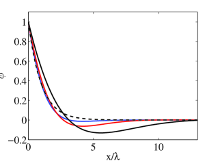
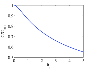
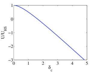
Figure 1: Low voltage solutions to the continuum model. a) Double layer structure at different values of $\delta_{c}$. Solutions are shown for $\delta_{c}=0$ (dashed) and $\delta_{c}=1,2,$ and $5$. b) Capacitance and c) slip velocity as a function of the correlation length scale, $\delta_{c}$.

IV.3.2 Solution for $\delta_{c}>1/2$, ”strong” correlation effects

When $\delta_{c}>1/2$ the analytical solution at low voltage has the form,

$$\phi(x)=\phi(0)e^{-k_{1}x}\left(\mathrm{cos}(k_{2}x)-A~{}\mathrm{sin}(k_{2}x)\right)$$ (39)

where

$$k_{1}=\frac{\sqrt{2\delta_{c}+1}}{2\delta_{c}},~{}k_{2}=\frac{\sqrt{2\delta_{c}-1}}{2\delta_{c}},~{}A=\frac{\sqrt{2\delta_{c}+1}(\delta_{c}-1)}{\sqrt{2\delta_{c}-1}(\delta_{c}+1)}$$

The capacitance of the double layer is,

$$\frac{C}{C_{DH}}=\frac{\sqrt{2\delta_{c}+1}}{\delta_{c}+1}$$ (40)

which decays with increasing correlations. The slip velocity is,

$$\frac{u(\infty)}{U_{HS}}=\left(1-\frac{\delta_{c}^{2}}{\delta_{c}+1}\right).$$ (41)

The slip velocity changes sign if $\delta_{c}$ is sufficiently large. In particular, there is an electro-osmotic flow reversal or electrokinetic charge inversion of the surface when the dimensionless correlation length exceeds the golden mean: $\delta_{c}>(1+\sqrt{5})/2=1.618$.

The form of the double layer becomes modified as $\delta_{c}$ increases. We find that the functional form consists of decaying sinusoids with a length scale provided explicitly by $k_{1}$ and $k_{2}$. At relatively large values of $\delta_{c}$ the length scale of the decay and the oscillations is approximately $\sqrt{2\delta_{c}}$.

IV.4 Numerical results

At low voltage, the solution has only one free parameter, the correlation length scale, $\delta_{c}$. The structure of the double layer as $\delta_{c}$ is varied is shown in Figure 1. We see that as the strength of the correlations is increased the double layer shows charge density oscillations. From the analytical solution we see that the oscillations emerge when $\delta_{c}$ is greater than 1/2. The length scale for the whole double layer also increases as the correlations are increased. From the analytical solution we can easily see at large $\delta_{c}$ that the size of the double layer grows with the square root of $\delta_{c}$. For small values of $\delta_{c}$ the results become indistinguishable from the classic Debye-Huckel solution.

In Figure 1 (b) we show the capacitance and (c) slip velocity as a function of $\delta_{C}$. We see a decrease in the slip velocity and the capacitance with increasing $\delta_{c}$. As correlation effects become stronger the flow is quenched and then reverses direction. Note that from the analytical solution that at $\delta_{c}=1$ that the flow velocity is half of $U_{HS}$ and the flow reverses when $\delta_{c}>0.618$. These values of $\delta_{c}$ are easily reached at high concentration in aqueous electrolytes, as we will soon see.

a)                                                    b)                                                   c)

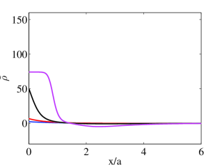
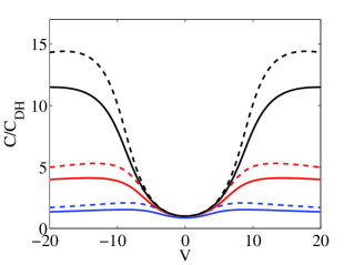
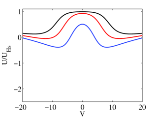
d)                                                    e)                                                   f)

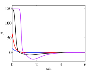
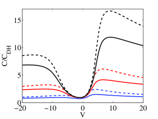
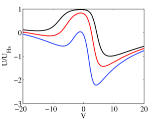
Figure 2: Example solutions for a 1:1 (a, b, and c) and 2:1 electrolyte (d, e, and f) with 0.3 nm ion sizes. (a) Double layer structure showing the charge density profiles at wall voltages of -1, -2, -5 and -10 in units of $k_{b}T/e$ for a 1 Molar concentration of cations. (b) Dimensionless capacitance as a function of voltage for concentration of 0.01 (black), 0.1 (red) and 1 (blue) molar from top to bottom. Corresponding solutions with no correlation effects ($\delta_{c}=0$) are shown as the dashed lines. (c) Dimensionless slip velocity as a function of voltage for concentration of 0.01 (black), 0.1 (red) and 1 (blue) molar. Without correlations the slip velocity is always 1. Figures (c), (d), and (e) are the same, only for the 2:1 system. The asymmetry is easily seen in the capacitance and slip velocity.

At higher applied voltage the structure of the solution changes dramatically as we show in Figure 2. Here we show sample solutions for a 1:1 and 2:1 electrolyte of 0.3 nm ions as the voltage is changed. In Figure 2a we show the structure of the double layer at different voltages at a cation concentration of 1 molar. Using the ion size as the correlation length scale and as the volume fraction then for the 1:1 system $\delta_{c}=0.988$, $\nu=0.0270$ and for the 2:1 system $\delta_{c}=1.71$, $\nu=0.0405$. As the voltage increases, the charge density at the wall saturates to a value determined by the steric constraints. This condensed layer of ions grows as the voltage is increase. Without the correlations effect the charge density would decay monotonically from the maximum value to zero far from the wall. However, with the correlation effects included in the model, the charge density oscillates and changes sign. These oscillations are more pronounced in 2:1 system when the divalent ions crowd the wall.

Turning to the capacitance in Figure 2b we find that correlation effects reduce the capacitance. The dimensionless capacitance is always 1 at zero voltage when $\delta_{c}=0$, however when $\delta_{c}>0$ the capacitance at zero voltage reduces according to Figure 1b. At higher voltage, the shape of the capacitance curve is similar to when $\delta_{c}=0$, the values are simply lower. This reduction in capacitance is consistent with previous work on steric constraints with the Bikerman model which found generally that the theory needed ion sizes that were bigger than one would expect physically to fit the experimental data Storey et al. (2008); Bazant et al. (2009a)

The most dramatic departure from the classical model comes when computing the slip velocity in Figure 2c. We see that at high concentration the model can predict reverse flow even at small voltages in the 2:1 system. At low concentration, we find that the model predicts classic slip at low voltage but predicts reverse flow as the voltage is increased even moderately. As the voltage is increased further, the model predicts the forward component of the flow begins to increase as the condensed layer grows. At high voltage the slip velocity for all concentrations begin to come together as the condensed layer begins to dominate the double layer structure.

These preliminary flow results must be interpreted with caution. The model currently does not account for changes in the viscosity of the solution near the wall in the condensed layer. It is also unclear (as it is in classical theory) where the slip plane should be placed. Recent work by Jiang and Qiao shows via molecular dynamics simulations that electroosmotic flow can be amplified by short wavelength hydrodynamics Jiang and Qiao (2012). These effects (and others) are not included in our model and may be required for more detailed comparisons with experimental data.

V Validation

V.1 Comparison with molecular simulations

In order to determine whether this model has validity in the context of aqueous electrolytes, we can compare the model predictions to those made by more sophisticated simulations such as Monte Carlo or Density Functional Theory (DFT). Monte Carlo simulations are often considered the standard for equilibrium chemistry while DFT has proven to quantitatively compare well against Monte Carlo at a much lower computational cost Gillespie et al. (2011). Our aim is to determine whether an even simpler continuum model can capture the same features.

In a prior paper we compared this correlations model to molecular dynamics simulations of ionic liquids Bazant et al. (2011). In that work we assumed that the potential at $x=0$ in the continuum theory was the potential offset from the wall by the radius of the ion. In comparisons to data for electrolyte solutions that follow, we find that here we obtain good results by taking the voltage at $x=0$ to be the electrode, i.e. not accounting for the radius of the ion as it approaches the surface.

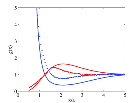
Figure 3: Comparison of the continuum model (solid lines) to Monte Carlo simulations of ref Boda et al. (2002). The conditions here are a 2:1 electrolyte with surface charge of -0.3 $\mathrm{C/m^{2}}$ and an ion diameter of 0.3 nm. The points are the Monte Carlo simulation and the solid lines are the continuum model.

In Figure 3 we compare the ion distributions, $g(x)=c(x)/c_{\infty}$, predicted by the continuum model to those predicted by Monte Carlo simulations of Boda et al Boda et al. (2002). The conditions here are a 2:1 electrolyte with surface charge of -0.3 $\mathrm{C/m^{2}}$ and an ion diameter of 0.3 nm. We find that the continuum model predicts much of the same structure as the Monte Carlo simulations, though the length scale of the oscillations and the amount of over-screening predicted by the continuum model is larger than seen in the simulations. Better agreement can be obtained by reducing the correlation length scale by about 50 percent. However, the classic electrokinetic model can only predict ion profiles which decay monotonically, so it is interesting that this extension for correlations effects can provide the basic double layer structure with no fitting parameters.

In Figure 4 a-b we compare the continuum model to the Monte Carlo simulations looking at the relationship between the double layer charge and electrode voltage. In a) we show results for a monovalent ion and in b) we show a 2:1 electrolyte at two different concentrations. The continuum model predicts the basic trends of the more complicated MC simulations, though under-predicts the voltage for a given charge. The inclusion of correlation effects brings the continuum results in better agreement with the MC simulations than when we only account for finite size effects.

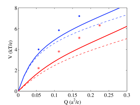
a) b)

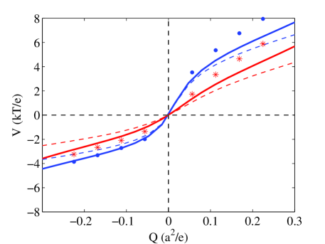
Figure 4: Comparison of the continuum model with correlations (solid lines) to Monte Carlo simulations of ref Boda et al. (2002) (points) and the continuum model with only steric effects (dashed lines). The ion diameter is 0.3 nm. In a) we show the result for a 1:1 electrolyte and in b) we show the result for a 2:1 electrolyte. The upper solid blue curve and dots is for 0.1 M and the lower red curve and ’*’ is for 1 M concentration.

In Figures 5 we compare the continuum model to results of density functional theory (DFT) simulations of Gillespie et al Gillespie et al. (2011) for a 2:1 electrolyte. In Figures 5 we show curves of constant voltage over a range of surface charge and concentration. The results with the continuum model are in reasonable agreement with the DFT results, especially at large concentrations and high charge. Importantly, the shape of these curves computed with DFT are well predicted by this simple continuum model. When $\delta_{c}=0$ and at high concentration, the continuum model qualitatively departs from the DFT results. What is interesting about the continuum model with correlations included is that there are no fit parameters.

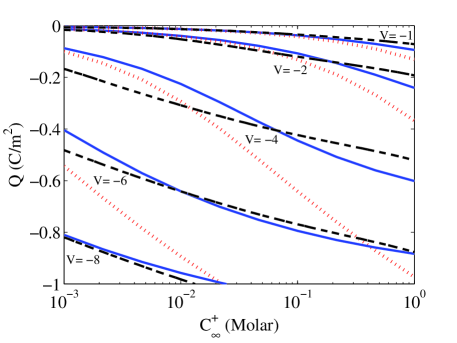
Figure 5: Comparison of the continuum model accounting for correlation effects (blue solid lines) to the DFT simulations of Gillespie et al Gillespie et al. (2011) (black dashed) to the continuum model with $\delta_{c}=0$ (red dotted lines). The ion diameter is 0.3 nm in the models and DFT.

V.2 Comparison with experiments

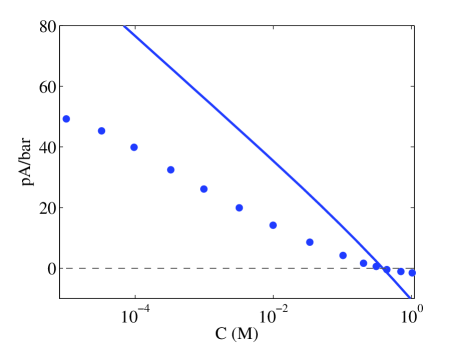
Figure 6: Comparison of the continuum model experimental nanochannel data of van der Heyden et al. (2006). The electrolyte is a 2:1 with an assumed ion size of 0.3 nm.

We can also compare the model to an experiment, rather than to other simulations, as a more definitive test. In Figure 6 we compare the model to the nanochannel electrokinetic data of van der Heyden et al. van der Heyden et al. (2006) as was done by Gillespie et al Gillespie et al. (2011). In the experiment a nanochannel with a characterized surface charge is driven by a pressure driven flow and the streaming current is measured. In this case the flow is driven by pressure and not electro-osmotically. To compute the streaming current we simply multiply our charge density profiles by the pressure driven velocity profile;

$$I=W\int_{0}^{H}\rho(x)u(x)dx$$ (42)

where $W$ is the channel width of 50 $\mu$m, $H$ is the channel height of 450 nm, and $u$ is the parabolic velocity profile. Since the double layer is so thin relative to the channel height of 450 nm, we can safely assume that the pressure driven velocity profile is locally linear at the wall; $du/dx=4\Delta PH/(L\eta)$ for Pouiselle flow. Thus to compute the current per unit pressure drop for pressure driven flow we calculate,

$$\frac{I}{\Delta P}=\frac{4WH}{L\eta}\int_{0}^{\infty}\rho(x)xdx.$$ (43)

The current per unit pressure as a function of concentration is plotted in Figure 6 comparing the continuum model to the experiment. The agreement is qualitatively correct and predicts a reversal in the current around the same concentration as seen in the experiments. The slower velocities at high concentration seen in the experiment is consistent with charge induced thickening, and increase in viscosity in a condensed layer of ions Bazant et al. (2009a). There is still uncertainty in application of this model for flow. It is unclear where the slip plane should sit and whether the solution viscosity near the wall should be taken as a constant. This uncertainty applies equally to the continuum model and the DFT simulations, as in those simulations the current is calculated in the same way it is here, only the charge profile is calculated via DFT in their work is used. More experimental data under controlled situations is needed for further testing predictions of flow.

We also briefly draw attention to induced-charge electro-osmotic flows (ICEO) Bazant et al. (2009a); Bazant and Squires (2010), where the new model may help to explain some puzzling experimental results (although we do not report any new simulations here). In particular, we (along with L. R. Edwards and M. S. Kilic) showed that flow reversal in AC electro-osmotic micro-pumps (consisting of interdigitated planar micro-electrode arrays) could be explained by a Bikerman-like model of the double layer, where the differential capacitance of the double layer decreases at high voltage Storey et al. (2008). A difficulty with this interperation of the experimental data, however, was the fact that the inferred ion size was far too large, whether considering a lattice gas or hard spheres. The problem could be alleviated by considering the possibility of reduction of the dielectric constant near the surface, and we speculated that correlation effects might further reduce the effective ion size in the model. From the present work, we can see that electrostatic correlations tend to reduce electro-osmotic flow while also lowering the double-layer differential capacitance. The former effect could be wholly or partly misinterpreted as a sign of charge-induced thickening (i.e. an increase in viscosity in a highly charged double layer that could also reduce the net electro-osmotic flow), while the latter could reduce the capacitance without invoking such strong steric effects with large effective ion sizes. Based on this evidence, it seems plausible that the new model might help to describe ICEO flows at high voltage and high salt concentration, which have otherwise resisted a complete theoretical understanding Bazant et al. (2009a).

VI Conclusions

We have developed a continuum model for electrokinetic phenomena that accounts for electrostatic correlations and applied this model to electro-osmotic flow and streaming current in aqueous electrolytes of high valence and high salt concentration at a flat, homogeneously charged surface. The model predicts the basic electric double layer structure that has been observed in Monte Carlo simulations; namely oscillations in the charge density and reversal of apparent charge of a surface based on electrokinetic flow. Without any fitting parameters, the continuum model which also includes finite ion size effects reproduces features of much more complicated theories and simulations. While the quantitative agreement between this model and Monte Carlo or DFT simulations is only approximate, the trends are much closer than found with the classical mean-field theory. As in the case of RTIL Bazant et al. (2011), it is remarkable that such a simple continuum theory can predict various subtle aspects of double layer structure and electrokinetic phenomena at the molecular scale.

References

- Lyklema (2003) J. Lyklema, Colloids and Surfaces A 222, 5 (2003).
- Bazant et al. (2009a) M. Z. Bazant, M. S. Kilic, B. Storey, and A. Ajdari, Advances in Colloid and Interface Science 152, 48 (2009a).
- Vlachy (1990) V. Vlachy, Annu. Rev. Phys. Chem. 50, 145 (1990).
- Hunter (2001) R. J. Hunter, Foundations of Colloid Science (Oxford University Press, Oxford, 2001).
- Lyklema (1995) J. Lyklema, Fundamentals of Interface and Colloid Science. Volume II: Solid-Liquid Interfaces (Academic Press Limited, San Diego, CA, 1995).
- Russel et al. (1989) W. B. Russel, D. Saville, and W. R. Schowalter, Colloidal Dispersions (Cambridge University Press, Cambridge, England, 1989).
- Stern (1924) O. Stern, Z. Elektrochem. 30, 508 (1924).
- Ramos et al. (1999) A. Ramos, H. Morgan, N. G. Green, and A. Castellanos, J. Colloid Interface Sci. 217, 420 (1999).
- Ajdari (2000) A. Ajdari, Phys. Rev. E 61, R45 (2000).
- Squires and Bazant (2004) T. M. Squires and M. Z. Bazant, J. Fluid Mech. 509, 217 (2004).
- Squires (2009) T. M. Squires, Lab on a Chip 9, 2477 (2009).
- Bazant and Squires (2010) M. Z. Bazant and T. M. Squires, Current Opinion in Colloid and Interface Science 15, 203 (2010).
- Kilic et al. (2007) M. S. Kilic, M. Z. Bazant, and A. Ajdari, Phys. Rev. E 75, 033702 (2007).
- Bikerman (1942) J. J. Bikerman, Philosophical Magazine 33, 384 (1942).
- Grimley and Mott (1947) T. B. Grimley and N. F. Mott, Discussions of the Faraday Society 1, 3 (1947).
- Storey et al. (2008) B. D. Storey, L. R. Edwards, M. S. Kilic, and M. Z. Bazant, Phys. Rev. E 77, 036317 (2008).
- Silvester and Compton (2006) D. Silvester and R. Compton, Z. Phys. Chem. 220, 1247 (2006).
- Freyland (2008) W. Freyland, Phys. Chem. Chem. Phys. 10, 923 (2008).
- Armand et al. (2009) M. Armand, F. Endres, D. R. MacFarlane, H. Ohno, and B. Scrosati, Nat. Mater. 8, 621 (2009).
- Ito et al. (2008) S. Ito, S. M. Zakeeruddin, P. Comte, P. Liska, D. Kuang, and M. Gratzel, Nat. Photonics 2, 693 (2008).
- Bai et al. (2008) Y. Bai, Y. Cao, J. Zhang, M. Wang, R. Li, P. Wang, S. M. Zakeeruddin, and M. Gratzel, Nat. Mater. 7, 626 (2008).
- Buzzeo et al. (2004) M. Buzzeo, R. Evans, and R.G.Compton, Chem. Phys. Chem. 5, 1106 (2004).
- Ye et al. (2001) C. Ye, W. Liu, Y. Chen, and L. Yu, Chem. Commun. 2244 (2001).
- Bhushan et al. (2008) B. Bhushan, M. Palacio, and B. Kinzig, J. Colloid Interface Sci. 317, 275 (2008).
- Kornyshev (2007) A. A. Kornyshev, J. Phys. Chem. B 111, 5545 (2007).
- Levin (2002) Y. Levin, Rep. Prog. Phys. 65, 1577 (2002).
- Bazant et al. (2011) M. Z. Bazant, B. D. Storey, and A. A. Kornyshev, Phys. Rev. Lett. 106, 046102 (2011).
- Bazant et al. (2005) M. Z. Bazant, K. T. Chu, and B. J. Bayly, SIAM J. Appl. Math. 65, 1463 (2005).
- Macdonald and Barlow (1962) J. R. Macdonald and C. A. Barlow, J. Chem. Phys. 36, 3062 (1962).
- di Caprio et al. (2003) D. di Caprio, Z. Borkowska, and J. Stafiej, J. Electroanal. Chem. 540, 17 (2003).
- Biesheuvel and van Soestbergen (2007) P. M. Biesheuvel and M. van Soestbergen, Journal of Colloid and Interface Science 316, 490 (2007).
- Carnahan and Starling (1969) N. F. Carnahan and K. E. Starling, J. Chem. Phys. 51, 635 (1969).
- Bazant et al. (2009b) M. Z. Bazant, M. S. Kilic, B. D. Storey, and A. Ajdari, New Journal of Physics 11, 075016 (2009b).
- Bockris and Reddy (1970) J. O. Bockris and A. K. N. Reddy, Modern Electrochemistry (Plenum, New York, 1970).
- Grahame (1950) D. C. Grahame, J. Chem. Phys. 18, 903 (1950).
- Macdonald (1987) J. R. Macdonald, J .Electroanal. Chem. 223, 1 (1987).
- Abrashkin et al. (2007) A. Abrashkin, D. Andelman, and H. Orland, Physical Review Letters 99, 077801 (2007).
- Hatlo et al. (2012) M. M. Hatlo, R. van Roij, and L. Lue, EPL 97 (2012).
- Tosi (1991) M. P. Tosi, Condensed Matter Physics Aspects of Electrochemistry (World Scientific, 1991), p. 68.
- Rovere and Tosi (1986) M. Rovere and M. P. Tosi, Rep. Prog. Phys. 49, 1001 (1986).
- Santangelo (2006) C. D. Santangelo, Physical Review E 73, 041512 (2006).
- Chen and Weeks (2006) Y.-G. Chen and J. D. Weeks, Proc. Nat. Acad. Sci. (USA) 103, 7560 (2006).
- Hatlo and Lue (2010) M. M. Hatlo and L. Lue, Europhysics Letters 89, 25002 (2010).
- Landau and Lifshitz (1984) L. D. Landau and E. M. Lifshitz, Electrodynamcis of Continuous Media (Pergammon, London, 1984), second edition ed.
- Kornyshev et al. (1978) A. A. Kornyshev, A. I. Rubinshtein, and M. A. Vorotyntsev, J. Phys. C.: Solid State Phys. 11, 3307 (1978).
- Kornyshev et al. (1982) A. A. Kornyshev, W. Schmickler, and M. A. Vorotyntsev, Phys. Rev. B 25, 5244 (1982).
- Hildebrandt et al. (2004) A. Hildebrandt, R. Blossey, S. Rjasanow, O. Kohlbacher, and H.-P. Lenhof, Phys. Rev. Lett. 93, 108104 (2004).
- Rottler and Krayenhoff (2009) J. Rottler and B. Krayenhoff, J. Phys.: Condens. Matter 21, 255901 (2009).
- Jiang and Qiao (2012) X. Jiang and R. Qiao, J. Phys. Chem. C 116, 1133 (2012).
- Gillespie et al. (2011) D. Gillespie, A. S. Khair, J. Bardhan, and S. Pennathur, J. Colloid and Int. Sci. 359, 520 (2011).
- Boda et al. (2002) D. Boda, W. R. Fawcett, D. Henderson, and S. Sokolowski, J. Chem. Phys. 11, 7170 (2002).
- van der Heyden et al. (2006) F. H. J. van der Heyden, D. Stein, K. Besteman, S. G. Lemay, and C. Dekker, Phys. Rev. Lett. 96 (2006).