An illustration of the light-front coupled-cluster method in quantum electrodynamics

Abstract

A field-theoretic formulation of the exponential-operator technique is applied to a nonperturbative Hamiltonian eigenvalue problem in electrodynamics, quantized in light-front coordinates. Specifically, we consider the dressed-electron state, without positron contributions but with an unlimited number of photons, and compute its anomalous magnetic moment. A simple perturbative solution immediately yields the Schwinger result of $\alpha/2\pi$. The nonperturbative solution, which requires numerical techniques, sums a subset of corrections to all orders in $\alpha$ and incorporates additional physics.

I Introduction

The light-front coupled-cluster (LFCC) method LFCClett is a nonperturbative scheme for the solution of field-theoretic Hamiltonian eigenvalue problems. It is based on light-front quantization Dirac ; DLCQreviews and the mathematics of the many-body coupled-cluster method CCorigin used in nuclear physics and quantum chemistry CCreviews . Here we give a brief introduction to the LFCC method and show how it can be applied to quantum electrodynamics LFCCqed .

The use of light-front quantization is crucial, in order to have well-defined Fock-state expansions and separation of internal and external momenta DLCQreviews . We define the coordinates as $x^{\pm}=t\pm z$, with $x^{+}$ the light-front time, and $\underline{x}=(x^{-},x,y)$. The light-front energy is $p^{-}=E-p^{z}$ and the momentum is $\underline{p}=(p^{+},\vec{p}_{\perp})$, with $p^{+}=E+p^{z}$ and $\vec{p}_{\perp}=(p^{x},p^{y})$. The mass-shell condition $p^{2}=m^{2}$ is then $p^{-}=\frac{m^{2}+p_{\perp}^{2}}{p^{+}}$, and the Hamiltonian eigenvalue problem is

$${\cal P}^{-}|\psi\rangle=\frac{M^{2}+P_{\perp}^{2}}{P^{+}}|\psi\rangle.$$ (1)

The eigenstate $|\psi\rangle$ is taken to be an eigenstate of light-front momentum and expanded in Fock states which are eigenstates of particle number as well as momentum. The coefficients of the Fock-state expansion are the wave functions; these satisfy a coupled set of integral equations derivable from (1).

The usual approach to approximation of this infinite system is to truncate Fock space at some fixed number of constituents and solve the remaining finite set of equations. However, Fock-space truncation can introduce a number of difficulties SecDep , in particular uncanceled divergences, which we wish to avoid. The LFCC method does avoid them.

The basic idea is to build the eigenstate as $|\psi\rangle=\sqrt{Z}e^{T}|\phi\rangle$ from a valence state $|\phi\rangle$ and an operator $T$. The $\sqrt{Z}$ factor maintains the normalization. The $T$ operator is constructed to include only terms that increase particle number but conserve all appropriate quantum numbers, such as momentum and charge. This leads to the definition of an effective Hamiltonian $\overline{{\cal P}^{-}}=e^{-T}{\cal P}^{-}e^{T}$, which can be constructed from the Baker–Hausdorff expansion $\overline{{\cal P}^{-}}={\cal P}^{-}+[{\cal P}^{-},T]+\frac{1}{2}[[{\cal P}^{-},T],T]+\cdots$. The eigenvalue problem can now be written as

$$P_{v}\overline{{\cal P}^{-}}|\phi\rangle=\frac{M^{2}+P_{\perp}^{2}}{P^{+}}|\phi\rangle,\;\;\;\;(1-P_{v})\overline{{\cal P}^{-}}|\phi\rangle=0,$$ (2)

where $P_{v}$ is a projection onto the valence sector. The first equation limits the eigenvalue problem to the valence sector; the second equation is an equation for the $T$ operator.

At this point, no approximation has been made and the problem remains of infinite size, because $T$ can contain an infinite number of terms. The approximation made in the LFCC method is to truncate $T$, rather than Fock space, and truncate $1-P_{v}$ to yield a finite set of equations sufficient to solve for the terms in $T$.

In the case of the dressed-electron state of QED LFCCqed , the valence state is the bare electron state. A first choice for $T$ is a term that invokes photon emission, and the corresponding truncation of $1-P_{v}$ is to allow only one additional photon. If we represent the Hamiltonian ${\cal P}^{-}$ by the graphs in Fig. 1(a),

(a)

(b)

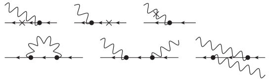
(c)

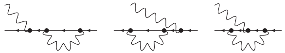
(d)

Figure 1: Graphs representing (a) the QED Hamiltonian ${\cal P}^{-}$, (b) the approximate $T$ operator, and the commutators (c) $[{\cal P}^{-},T]$ and (d) $[[{\cal P}^{-},T],T]$. Positron contributions are neglected, and a cross represents a kinetic energy contribution. In (c) and (d), only terms that contribute to the given truncation of $1-P_{v}$ are kept.

this choice for $T$ can be represented by the graph in Fig. 1(b). The commutators that enter the Baker–Hausdorff expansion are represented in Figs. 1(c) and (d). A key result is that the self-energy loops that appear in Fig. 1 are all the same, with no spectator or sector dependence.

The truncation of $1-P_{v}$ limits the number of commutators that need to be calculated, because each factor of $T$ increases the particle number by one. The QED Hamiltonian includes terms that decrease particle number by no more than one; therefore, two commutators are sufficient when $1-P_{v}$ limits the increase to one.

II Application to QED

To be more explicit, we give some details of the application of the LFCC method to QED LFCCqed . The Pauli–Villars regulated Lagrangian is ArbGauge

$${\cal L} = \sum_{i=0}^{2}(-1)^{i}\left[-\frac{1}{4}F_{i}^{\mu\nu}F_{i,\mu\nu}+\frac{1}{2}\mu_{i}^{2}A_{i}^{\mu}A_{i\mu}-\frac{1}{2}\zeta\left(\partial^{\mu}A_{i\mu}\right)^{2}\right]$$

$$+\sum_{i=0}^{2}(-1)^{i}\bar{\psi_{i}}(i\gamma^{\mu}\partial_{\mu}-m_{i})\psi_{i}-e\bar{\psi}\gamma^{\mu}\psi A_{\mu},$$

with $\psi=\sum_{i=0}^{2}\sqrt{\beta_{i}}\psi_{i}$, $A_{\mu}=\sum_{i=0}^{2}\sqrt{\xi_{i}}A_{i\mu}$, and $F_{i\mu\nu}=\partial_{\mu}A_{i\nu}-\partial_{\nu}A_{i\mu}$. Here $i=0$ corresponds to a physical field and $i=1,2$ to Pauli–Villars (PV) fields. The gauge-fixing parameter $\zeta$ is left arbitrary. The coupling coefficients are constrained by $\xi_{0}=1$, $\sum_{i=0}^{2}(-1)^{i}\xi_{i}=0$, $\beta_{0}=1$, $\sum_{i=0}^{2}(-1)^{i}\beta_{i}=0$, and by restoration of chiral symmetry ChiralLimit and a zero photon mass VacPol . Neglecting positron contributions, the Hamiltonian is

$${\cal P}^{-}=\sum_{is}\int d\underline{p}\frac{m_{i}^{2}+p_{\perp}^{2}}{p^{+}}(-1)^{i}b_{is}^{\dagger}(\underline{p})b_{is}(\underline{p})+\sum_{l\lambda}\int d\underline{k}\frac{\mu_{l\lambda}^{2}+k_{\perp}^{2}}{k^{+}}(-1)^{l}\epsilon^{\lambda}a_{l\lambda}^{\dagger}(\underline{k})a_{l\lambda}(\underline{k})$$

$$+\sum_{ijl\sigma s\lambda}\int dyd\vec{k}_{\perp}\int\frac{d\underline{p}}{\sqrt{16\pi^{3}p^{+}}}$$

$$\rule{21.68121pt}{0.0pt}\times\left\{h_{ijl}^{\sigma s\lambda}(y,\vec{k}_{\perp})a_{l\lambda}^{\dagger}(yp^{+},y\vec{p}_{\perp}+\vec{k}_{\perp})b_{js}^{\dagger}((1-y)p^{+},(1-y)\vec{p}_{\perp}-\vec{k}_{\perp})b_{i\sigma}(\underline{p})\right.$$

$$\left.\rule{28.90755pt}{0.0pt}+h_{ijl}^{\sigma s\lambda*}(y,\vec{k}_{\perp})b_{i\sigma}^{\dagger}(\underline{p})b_{js}((1-y)p^{+},(1-y)\vec{p}_{\perp}-\vec{k}_{\perp})a_{l\lambda}(yp^{+},y\vec{p}_{\perp}+\vec{k}_{\perp})\right\},$$

with $\epsilon^{\lambda}=(-1,1,1,1)$ and the $h_{ijl}^{\sigma s\lambda}$ known vertex functions LFCCqed . The $b_{is}^{\dagger}$ create fermions of type $i$ and spin $s$, and the $a_{l\lambda}^{\dagger}$ create photons of type $l$ and polarization $\lambda$.

The valence state for the dressed electron is just the single-electron state $|\phi_{a}^{\pm}\rangle=\sum_{i}z_{ai}b_{i\pm}^{\dagger}(\underline{P})|0\rangle$, where $a=0,1$; there are two possible states because the valence sector includes the PV electron. The approximate $T$ operator is

$$T = \sum_{ijls\sigma\lambda}\int dyd\vec{k}_{\perp}\int\frac{d\underline{p}}{\sqrt{16\pi^{3}}}\sqrt{p^{+}}t_{ijl}^{\sigma s\lambda}(y,\vec{k}_{\perp})$$

$$\rule{36.135pt}{0.0pt}\times a_{l\lambda}^{\dagger}(yp^{+},y\vec{p}_{\perp}+\vec{k}_{\perp})b_{js}^{\dagger}((1-y)p^{+},(1-y)\vec{p}_{\perp}-\vec{k}_{\perp})b_{i\sigma}(\underline{p}).$$

The effective Hamiltonian can then be computed LFCCqed and used.

The eigenvalue problem in the valence sector $P_{v}\overline{{\cal P}^{-}}P_{v}|\phi_{a}^{\pm}\rangle=\frac{M_{a}^{2}+P_{\perp}^{2}}{P^{+}}|\phi_{a}^{\pm}\rangle$ becomes the 2$\times$2 matrix equation

$$m_{i}^{2}z_{ai}^{\pm}+\sum_{j}I_{ij}z_{aj}^{\pm}=M_{a}^{2}z_{ai}^{\pm}.$$ (6)

Here we have the self-energy contribution

$$I_{ji}=(-1)^{i}\sum_{i^{\prime}ls\lambda}(-1)^{i^{\prime}+l}\epsilon^{\lambda}\int\frac{dyd\vec{k}_{\perp}^{\,\prime}}{16\pi^{3}}h_{ji^{\prime}l}^{\sigma s\lambda*}(y,\vec{k}_{\perp})t_{ii^{\prime}l}^{\sigma s\lambda}(y,\vec{k}_{\perp}).$$ (7)

The equation for the $T$ operator, obtained from a projection onto the one-electron/one-photon sector, reduces to

$$\sum_{i}(-1)^{i}z_{ai}^{\pm}\left\{h_{ijl}^{\pm s\lambda}(y,\vec{k}_{\perp})+\left[\frac{m_{j}^{2}+k_{\perp}^{2}}{1-y}+\frac{\mu_{l\lambda}^{2}+k_{\perp}^{2}}{y}-m_{i}^{2}\right]t_{ijl}^{\pm s\lambda}(y,\vec{k}_{\perp})\right.$$

$$\left.+\frac{1}{2}V_{ijl}^{\pm s\lambda}(y,\vec{k}_{\perp})+\frac{1}{2}\sum_{i^{\prime}}\frac{I_{ji^{\prime}}}{1-y}t_{ii^{\prime}l}^{\pm s\lambda}(y,\vec{k}_{\perp})-\sum_{j^{\prime}}(-1)^{i+j^{\prime}}t_{j^{\prime}jl}^{\pm s\lambda}(y,\vec{k}_{\perp})I_{j^{\prime}i}\right\}=0,$$

with $V_{ijl}^{\pm s\lambda}$ a vertex correction LFCCqed .

To partially diagonalize in flavor, we define $C_{abl}^{\pm s\lambda}(y,\vec{k}_{\perp})=\sum_{ij}(-1)^{i+j}z_{ai}^{\pm}\tilde{z}_{bj}^{\pm}t_{ijl}^{\pm s\lambda}(y,\vec{k}_{\perp})$ and use analogous definitions for $H$, $I$, and $V$. Here the $\tilde{z}_{bj}$ are the left-hand analogs of the $z_{ai}$, which arise because the effective Hamiltonian is not Hermitian. The equation for $C_{abl}^{\pm s\lambda}$ is then

$$\left[M_{a}^{2}-\frac{M_{b}^{2}+k_{\perp}^{2}}{1-y}-\frac{\mu_{l\lambda}^{2}+k_{\perp}^{2}}{y}\right]C_{abl}^{\pm s\lambda}(y,\vec{k}_{\perp})$$ (9)

$$=H_{abl}^{\pm s\lambda}(y,\vec{k}_{\perp})+\frac{1}{2}\left[V_{abl}^{\pm s\lambda}(y,\vec{k}_{\perp})-\sum_{b^{\prime}}\frac{I_{bb^{\prime}}}{1-y}C_{ab^{\prime}l}^{\pm s\lambda}(y,\vec{k}_{\perp})\right].$$

This is to be solved simultaneously with valence sector equations, which depend on $C/t$ through the self-energy matrix $I$. Notice that the physical mass $M_{b}$ has replaced the bare mass in the kinetic energy term, without use of sector-dependent renormalization SecDep .

As an example of a calculation of a physical quantity from the dressed-electron state, we consider the anomalous magnetic moment. The moment can be obtained from the spin-flip matrix element of the current $J^{+}=\overline{\psi}\gamma^{+}\psi$ coupled to a photon of momentum $q$. Computation of such matrix elements requires solution of a left-hand eigenvalue problem for the effective Hamiltonian; details are given in LFCCqed . When solved perturbatively, this yields the standard Schwinger result Schwinger of $\alpha/2\pi$ for the anomalous moment. The full (numerical) solution will include all $\alpha^{2}$ contributions without electron-positron pairs and partial summation of higher orders.

III Summary

The LFCC method provides a new approach to the nonperturbative solution of light-front Hamiltonian eigenvalue problems, one that avoids Fock-space truncation and its attendant difficulties. The use of the method is illustrated here in the case of QED LFCCqed and elsewhere for a soluble model LFCClett . The approximation made by truncating the $T$ operator is systematically improvable by the addition of terms classified by the net number of particles created and by the total number of annihilation operators. The self-energy corrections generated in the effective Hamiltonian are found to be sector and spectator independent.

For QED there are a number of extensions to consider beyond the present application. To include positrons, we must first study the dressed-photon state, in order to set the photon coupling coefficient at zero photon mass, and then include pairs in the dressed-electron state. Once these eigenstates are computed, we can consider true bound states, such as muonium and positronium.

Beyond QED, we can, of course, consider QCD. In fact, nonperturbative methods are not particularly important for QED and other weak-coupling theories, and are instead intended for QCD. There we can begin with light-front holographic QCD hQCD before considering the full theory. It is also interesting to consider simpler theories with spontaneous symmetry breaking, to better understand the LFCC method in such a context.

- (1) S.S. Chabysheva and J.R. Hiller, Phys. Lett. B 711, 417–422 (2012).
- (2) P.A.M. Dirac, Rev. Mod. Phys. 21, 392–399 (1949).
- (3) For reviews of light-cone quantization, see M. Burkardt, Adv. Nucl. Phys. 23, 1–74 (2002); S.J. Brodsky, H.-C. Pauli, and S.S. Pinsky, Phys. Rep. 301, 299–486 (1998).
- (4) F. Coester, Nucl. Phys. 7, 421–424 (1958); F. Coester and H. Kümmel, Nucl. Phys. 17, 477–485 (1960).
- (5) For reviews of the many-body coupled-cluster method, see R.J. Bartlett and M. Musial, Rev. Mod. Phys. 79, 291–352 (2007); T.D. Crawford, and H.F. Schaefer, Rev. Comp. Chem. 14, 33–136 (2000); R. Bishop, A.S. Kendall, L.Y. Wong, and Y. Xian, Phys. Rev. D 48, 887–901 (1993); H. Kümmel, K.H. Lührmann, and J.G. Zabolitzky, Phys. Rep. 36, 1–63 (1978).
- (6) S.S. Chabysheva and J.R. Hiller, “An application of the light-front coupled-cluster method to the nonperturbative solution of QED,” arXiv:1203.0250 [hep-ph].
- (7) S.S. Chabysheva and J.R. Hiller, Ann. Phys. 325, 2435–2450 (2010).
- (8) S.S. Chabysheva and J.R. Hiller, Phys. Rev. D 84, 034001:1–13 (2011).
- (9) S.S. Chabysheva and J.R. Hiller, Phys. Rev. D 79, 114017:1–11 (2009).
- (10) S.S. Chabysheva and J.R. Hiller, Phys. Rev. D 82, 034004:1–8 (2010).
- (11) J. Schwinger, Phys. Rev. 73 (1948) 416–417; Phys. Rev. 76 (1949) 790–817.
- (12) G.F. de Teramond, and S.J. Brodsky, Phys. Rev. Lett. 102, 081601:1–4 (2009).