Suppression of Hyperfine Dephasing by Spatial Exchange of Double Quantum Dots

Abstract

We examine the logical qubit system of a pair of electron spins in double quantum dots. Each electron experiences a different hyperfine interaction with the local nuclei of the lattice, leading to a relative phase difference, and thus decoherence. Methods such as nuclei polarization, state narrowing, and spin-echo pulses have been proposed to delay decoherence. Instead we propose to suppress hyperfine dephasing by adiabatic rotation of the dots in real space, leading to the same average hyperfine interaction. We show that the additional effects due to the motion in the presence of spin-orbit coupling are still smaller than the hyperfine interaction, and result in an infidelity below $10^{-4}$ after ten decoupling cycles. We discuss a possible experimental setup and physical constraints for this proposal.

I Introduction

In recent years there has been great interest in the prospect of using scalable solid state devices to implement quantum two-level systems(qubits) for potential applications such as quantum computation. One promising candidate for a qubit is a pair of electron spins in quantum dots, which forms a fault-tolerant subspace that is immune to collective decoherence.Levy (2002) However, each electron is still subject to the local hyperfine interaction from the nuclear spins of the lattice, which leads to dephasing of the individual electron spins.Burkard et al. (1999) There have been several proposals to suppress this dephasing such as nuclear polarization,Burkard et al. (1999); Khaetskii et al. (2003); Gullans et al. (2010) state narrowing,Klauser et al. (2006) and spin-echo pulse correction.Khodjasteh and Lidar (2005); Zhang et al. (2007) While improved coherence has been experimentally demonstrated using these techniques, the coherence times desired for applications have proven very difficult to achieve. For example, pumping methods have been used to partially polarize nuclei, but the nearly full polarization needed has yet to be achieved.Klauser et al. (2006); Imamoḡlu et al. (2003); Taylor et al. (2003); Reilly et al. (2008)

Promising results have been shown using spin-echo sequences through the exchange interaction between two spins.Petta et al. (2005); Barthel et al. (2010); van Weperen et al. (2011) The exchange is controlled by lowering the tunneling barrier between the two quantum dots using quickly-controlled electric gates. This leads to Rabi oscillations; a single $\pi$-pulse corresponds to exchanging the two spins. Sequences of such pulses effectively couple both spins to the same average hyperfine interaction resulting in improved coherence times. While several echo sequences can be performed using this exchange, it is likely that the electrical gate noise and spatial variations in the Overhauser field remain the dominant sources of dephasing.Barthel et al. (2010)

Rather than relying on interdot tunneling, we propose using a spatial exchange of the two quantum dots, allowing the two electrons to traverse the same path, spending the same time coupled to the local nuclei, as shown in Figure 1. Compared to exchange via tunneling, ideally, this should eliminate the effect of the electrical gate noise. On the other hand, in the presence of spin-orbit coupling, such a motion of electrons may introduce additional errors. In this manuscript we analyze how these errors depend on the parameters of the motion and discuss the constraints and possible parameters for potential implementation of this proposal.

Figure 1: Suggested electrode geometry for a rotating double-quantum-dot qubit with top and bottom gates in different shades of gray. Exchange gates via real space rotation, as opposed to tunneling, are expected to strongly reduce the qubit sensitivity to charge noise.

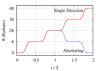
Figure 2: Time dependent adiabatic trajectories used in the simulations. Plotted is the position of the first dot parametrized in terms of the angle $\theta$ as a function of time $t$. The angle-dependent positions were defined as a sum of properly scaled and shifted hyperbolic tangents. Single direction rotations suppress the effect of a static Overhauser field but not of a time-varying one. Longer rotation sequences like alternating forward-and-back suppress the effect of a linear in time Overhauser field. Arbitary rotations on the Bloch sphere may be accomplished using additional operations when the dot is stationary, corresponding to the flat segments in the sequence.

We note that a similar setup with spatial exchange of electrostatically-defined quantum dots has been discussed in relation to holonomic quantum computation.Golovach et al. (2010); Shitade et al. (2010) However, the corresponding coherence estimates have been done in the absence of a magnetic field. Here we focus on the parameter range characteristic of double-quantum-dot qubits and take into account typical magnetic fields of order $\gtrsim 0.1$ T.

The outline of the paper is as follows. We define the Hamiltonian of the double-quantum-dot qubit with spatial exchange in Sec. II, derive the effective spin-only Hamiltonain for a single spin in a moving quantum dot in Sec. III, and calculate the single-qubit fidelity associated with a sequence of double-dot rotations in Sec. IV. We discuss simulations of a possible protocol in Sec. V, and the constraints and corresponding characteristic time and distance scales in Sec. VI, and conclude with Sec. VII.

II Setup

We envision a qubit formed by a pair of quantum dots electrostatically defined in a III-V semiconductor (e.g., GaAs/AlGaAs) heterostructure using a system of top and bottom gates similar to that illustrated in Fig. 1. We take the parameters of the dots to be similar to the experimental ones.  Petta et al. (2005); Barthel et al. (2010); van Weperen et al. (2011) Specifically, each dot contains a single electron, with a typical dot-size quantization energy $\hbar\omega_{d}\sim 1$meV. The qubit is defined as the subspace of the singlet and $m_{s}=0$ triplet states of the two electrons. The triplet degeneracy is removed by a uniform, constant magnetic field $B_{0}$ of at least $\sim 0.1$T applied perpendicular to the sample, which creates a Zeeman gap of $\Delta\sim 2.5$ µeV. The electrons interact with $N\sim 10^{6}$ spins of the lattice nuclei, leading to a different local hyperfine interaction for each electron. We will approximate this as a Zeeman interaction with a random, fluctuating, non-uniform magnetic “Overhauser” field $B_{\text{N}}\sim 1$mT.

To prevent dephasing, both quantum dots will be moved along the same trajectory in a time much shorter than the relaxation time of the nuclear spins, $t_{\text{nuc}}\sim 100$ µs, so we can assume that the Overhauser field is quasi-static. In order to reduce the sensitivity to charge noise the distance between the dots must be significantly greater than the size of each quantum dot, $a\sim 100$nm. Due to this spatial separation between the dots, we can treat the Hamiltonian of each electron separately,

$$H=H_{\text{d}}(\mathbf{r}_{0})+H_{\text{Z}}+V_{\text{Z}}(\mathbf{r},t)+H_{\text{SO}}+V(\mathbf{r},t).$$ (1)

Here the dot Hamiltonian is given by

$$H_{\text{d}}(\mathbf{r}_{0})=\frac{p^{2}}{2m}+U(\mathbf{r}-\mathbf{r}_{0}(t)),$$ (2)

with the canonical momentum $\mathbf{p}=\mathbf{P}+e\mathbf{A}/c$ and the confining potential $U$ centered at $\mathbf{r}_{0}\equiv\mathbf{r}_{0}(t)$; the Zeeman Hamiltonians for the externally-applied and Overhauser fields are respectively

$$H_{\text{Z}} =\frac{g\mu_{\text{B}}}{2}\mathbf{B}_{0}\cdot\boldsymbol{\sigma},$$ (3)

$$V_{\text{Z}}(\mathbf{r},t) =\frac{g\mu_{\text{B}}}{2}\mathbf{B}_{\text{N}}(\mathbf{r},t)\cdot\boldsymbol{\sigma},$$ (4)

and the spin-orbit Hamiltonian is given by

$$H_{\text{SO}}=\sigma^{i}C^{ij}p^{j}.$$ (5)

The last term, $V\biglb(\mathbf{r},t\bigrb)$, accounts for additional effects originating from disorder, variation of the dot potential as it moves due to imperfections of the confining potential, as well as phonons. The spin orbit coupling coefficients $C_{ij}$ in Eq. (5) incorporate both Dresselhaus (originating from the lack of the inversion symmetry of the lattice) with $C^{yy}=-C^{xx}=\beta$, and Rashba terms (structural inversion asymmetry due to the quantum well) with $C^{xy}=-C^{yx}=\alpha$. This specific form assumes that the growth of the semiconductor heterostructure and the quantum well asymmetry are in the positive $z$ direction,Silsbee (2004); Zawadzki and Pfeffer (2004) so all the matrix elements that involve $z$ are zero.

For numerical estimates we will use the effective electron mass $m\sim 0.067m_{\text{e}}$, and assume $\alpha\simeq\beta$ with values ranging from $10^{3}$ to $10^{4}$ m/s, as appropriate for typical GaAs heterostructures.Silsbee (2004) Based on the above values, we have $m\beta^{2}\ll g\mu_{\text{B}}B\ll\hbar\omega_{\text{d}}$, so we will ignore terms quadratic in the spin-orbit coupling for the following analysis.

III Effective single-dot Hamiltonian

We now go into the moving reference frame of the dot using the translation operator

$$\Psi(t) \to e^{-\frac{i}{\hbar}\mathbf{P}\cdot\mathbf{r}_{o}(t)}\Psi(t),$$ (6)

$$H \to e^{\frac{i}{\hbar}\mathbf{P}\cdot\mathbf{r}_{o}(t)}He^{-\frac{i}{\hbar}\mathbf{P}\cdot\mathbf{r}_{o}(t)}-\mathbf{v}_{0}(t)\cdot\mathbf{P},$$ (7)

which introduces the additional term proportional to the dot’s velocity, $\mathbf{v}_{0}\equiv\dot{\mathbf{r}}_{0}$, and removes the $\mathbf{r}_{0}$ from the confining potential, $U(\mathbf{r}-\mathbf{r}_{0})\to U(\mathbf{r})$. This also affects the vector potential, $\mathbf{A(r)\to A(r+r}_{0})$, in the dot Hamiltonian and spin-orbit term, which can be reversed with an appropriate gauge transformation. We select the symmetric gauge, $\mathbf{A}(\mathbf{r}+\mathbf{r}_{0})=\frac{1}{2}\mathbf{B}\times(\mathbf{r}+\mathbf{r}_{0})$, and transform $\mathbf{A}\to\mathbf{A}+\mathbf{\nabla}f$ with $f=-\frac{1}{2}\mathbf{r}\cdot(\mathbf{B}\times\mathbf{r}_{0})$ which results in

$$\Psi \to\Psi\,\exp(-\frac{ie}{\hbar c}f),$$ (8)

$$\mathbf{P} \to\mathbf{P}-\frac{e}{c}\mathbf{\nabla}f.$$ (9)

These transformations introduce two additional terms in the time-dependent Schrödinger equation $i\hbar\partial\Psi/\partial t=H\Psi$. The first term, $-({e}/{2c})\mathbf{v}_{0}\cdot(\mathbf{B}\times\mathbf{r}_{0})$, arises when Eq. (9) is substituted into the $-\mathbf{v}_{0}(t)\cdot\mathbf{P}$ term in Eq. (7). The second term, $-({e}/{2c})\mathbf{r}\cdot(\mathbf{B}\times\mathbf{v}_{0})$, appears on the left hand side as a result of taking the time derivative of the exponent in Eq. (8). These two terms can be moved to one side of the equation and combined using the cyclic property of the mixed product:

$$-\frac{e}{2c}\mathbf{v}_{0}\cdot(\mathbf{B}\times\mathbf{r}_{0})+\frac{e}{2c}\mathbf{r}\cdot(\mathbf{B}\times\mathbf{v}_{0})=-\frac{e}{2c}\mathbf{v}_{0}\cdot\mathbf{B}\times(\mathbf{r}+\mathbf{r}_{0})$$ (10)

which is precisely the vector potential term in $-\mathbf{v}_{0}\cdot\mathbf{p}$. This leads to the moving-frame Hamiltonian

$${H}=H_{\text{d}}+H_{\text{Z}}+H_{\text{SO}}+V(\mathrm{r}+\mathbf{r}_{0}(t),t)\\ +V_{\text{Z}}(\mathrm{r}+\mathbf{r}_{0}(t),t)-\mathbf{v}_{0}\cdot\mathbf{p}.$$ (11)

Following Golovach et al.Golovach et al. (2004), we now perform a canonical transformation $H\to e^{S}He^{-S}\simeq(1+S)H(1-S)=H+[S,H]$, where S is anti-Hermitian and chosen to eliminate the original spin-orbit term. We split $S=S_{0}+S_{1}$ such that

$$[S_{0},H_{\text{d}}]+H_{\text{SO}} =0,$$ (12)

$$[S_{1},H_{\text{d}}]+[S_{0},H_{\text{Z}}] =0,$$ (13)

and choose

$$S_{0}=\frac{im}{\hbar}\sigma^{i}C^{ij}r^{j},$$ (14)

which satisfies Eq. (12). This can be verified, noting that $S_{0}$ has no momentum dependence so it clearly commutes with the confining potential, and

$$\left[\frac{im}{\hbar}\sigma^{i}C^{ij}r^{j},\frac{p^{2}}{2m}\right] = \frac{i}{\hbar}\sigma^{i}C^{ij}[r^{j},p^{k}]p^{k}$$ (15)

$$= -\sigma^{i}C^{ij}p^{j}.$$

With $S_{0}$ known, we use Eq. (13) to define $S_{1}$,

$$[H_{d},S_{1}] =\, [S_{0},H_{\text{Z}}]=\frac{img\mu_{\text{B}}}{2\hbar}C^{ij}r^{j}[\sigma^{i},\sigma^{k}]B^{k}_{0}$$ (16)

$$=\, -\frac{mg\mu_{\text{B}}}{\hbar}C^{ij}r^{j}\epsilon^{ikl}B^{k}_{0}\sigma^{l}$$

$$=\, -\frac{g\mu_{\text{B}}}{2}\mathbf{Q}\cdot(\mathbf{B}_{0}\times\boldsymbol{\sigma})$$

$$=\, \frac{g\mu_{\text{B}}}{2}(\mathbf{B}_{0}\times\mathbf{Q})\cdot\boldsymbol{\sigma},$$

where $Q^{i}\equiv(2m/\hbar)C^{ij}r^{j}$. This equation can be written in terms of the electron’s orbital states $|n\rangle$ in the dot potential,

$$\langle n|[H_{d},S_{1}]|m\rangle=\, (S_{1})_{nm}(E_{n}-E_{m})$$

$$=\, \frac{g\mu_{\text{B}}}{2}\boldsymbol{\sigma}\cdot(\mathbf{B}_{0}\times\langle\mathbf{Q}\rangle_{nm}).$$ (17)

As long as the relevant dot quantization energies are non-degenerate, $E_{n}\neq E_{m}$, we have

$$(S_{1})_{nm} =\frac{g\mu_{\text{B}}}{2}\boldsymbol{\sigma}\cdot\frac{(\mathbf{B}_{0}\times\langle\mathbf{Q}\rangle_{nm})}{E_{n}-E_{m}}$$

$$=\frac{g\mu_{\text{B}}}{2}\boldsymbol{\sigma}\cdot\mathbf{W}_{nm},$$ (18)

where we defined

$$\mathbf{W}_{nm}\equiv\frac{\mathbf{B}_{0}\times\langle\mathbf{Q}\rangle_{nm}}{E_{n}-E_{m}}.$$ (19)

Expanding the canonical transformation to first order in the spin-orbit parameter contained in $S_{0}$ and $S_{1}$, we obtain the transformed Hamiltonian

$$\bar{H}\simeq H+[S_{0},V_{\text{Z}}]-[S_{0},\mathbf{v}_{0}\cdot\mathbf{p}]+[S_{1},V]\\ +[S_{1},H_{\text{Z}}]-[S_{1},\mathbf{v}_{0}\cdot\mathbf{p}]+[S_{1},V_{\text{Z}}]$$ (20)

Using the definition of $S_{0}$, the first two commutators are

$$\frac{img\mu_{\text{B}}}{2\hbar}C^{ij}r^{j}[\sigma^{i},\sigma^{k}]B_{\text{N}}^{k} =-\frac{mg\mu_{\text{B}}}{\hbar}C^{ij}r^{j}(\epsilon^{ikl}B_{\text{N}}^{k}\sigma^{l})$$

$$=\frac{g\mu_{\text{B}}}{2}(\mathbf{B}_{\text{N}}\times\mathbf{Q})\cdot\boldsymbol{\sigma}$$ (21)

and

$$-\frac{im}{\hbar}\sigma^{i}C^{ij}[r^{j},p^{k}]v_{0}^{k}=m\sigma^{i}C^{ij}v_{0}^{j}=\frac{1}{2}\mathbf{Q}_{\text{v}}\cdot\boldsymbol{\sigma},$$ (22)

respectively, with $Q_{\text{v}}^{i}\equiv 2mC^{ij}v_{0}^{j}$ defined analogously to $Q^{i}$. We now define the effective spin Hamiltonian by projecting onto the orbital ground state, $H_{S}\equiv\langle 0|\bar{H}|0\rangle$. This allows us to express the remaining commutators in the transformed Hamiltonian using the definition of $S_{1}$. The first commutator involving $S_{1}$ in Eq. (20) is simplified by explicitly writing out the commutator and inserting a complete set of states,

$$\langle 0|S_{1}V|0\rangle- \langle 0|VS_{1}|0\rangle$$

$$= \sum_{n>0}\langle 0|S_{1}|n\rangle\langle n|V|0\rangle-\langle 0|V|n\rangle\langle n|S_{1}|0\rangle$$

$$= \sum_{n>0}(S_{1})_{0n}V_{n0}-V_{0n}(S_{1})_{n0}.$$ (23)

We assume $V$ to have no momentum dependence, so it commutes with $S_{1}$ and we can reverse the order of the second term above. Since $S_{1}$ is anti-Hermitian, while $V$ is Hermitian,

$$\langle 0|S_{1}V|0\rangle- \langle 0|VS_{1}|0\rangle$$

$$= 2\sum_{n>0}(S_{1})_{0n}V_{n0}$$

$$= g\mu_{\text{B}}\boldsymbol{\sigma}\cdot\sum_{n>0}\mathbf{W}_{0n}V_{n0}.$$ (24)

This technique can be used on the remaining terms in Eq. (20). The second term involving $S_{1}$ in Eq. (20) vanishes because

$$(H_{\text{Z}})_{n0}=\frac{g\mu_{\text{B}}}{2}\boldsymbol{\sigma}\cdot\langle n|\mathbf{B}_{0}|0\rangle=0.$$ (25)

However, the final commutator in Eq. (20) contains the terms

$$(S_{1})_{0n}(V_{\text{Z}})_{n0}-(V_{\text{Z}})_{0n}(S_{1})_{n0},$$ (26)

which do not commute because they contain two spin terms, but can be treated using the spin identity

$$(\boldsymbol{\sigma}\cdot\mathbf{a})(\boldsymbol{\sigma}\cdot\mathbf{b})=\mathbf{a}\cdot\mathbf{b}+i\boldsymbol{\sigma}\cdot(\mathbf{a}\times\mathbf{b}).$$ (27)

The first term in Eq. (26) becomes

$$\left(\frac{g\mu_{\text{B}}}{2}\right)^{2}\{\mathbf{W}_{0n}\cdot(\mathbf{B_{\text{N}}})_{n0}+i\boldsymbol{\sigma}\cdot[\mathbf{W}_{0n}\times(\mathbf{B_{\text{N}}})_{n0}]\},$$ (28)

and the second term looks quite similar, except the anti-commutator of the cross product causes the spin dependent term to cancel with the one above, while the spin-indepedent terms is doubled. The Hamiltonian contains several of these spin-independent terms that can be taken as constants. The effective spin Hamiltonian, up to a constant, can now be written simply as

$$H_{S}={1\over 2}\hbar\left[\boldsymbol{\omega}_{0}+\boldsymbol{\omega}_{1}(t)\right]\cdot\boldsymbol{\sigma},$$ (29)

where

$$\boldsymbol{\omega}_{0}=\frac{g\mu_{\text{B}}}{\hbar}\mathbf{B}_{0},$$ (30)

is the Larmor frequency, and the time-dependent term $\omega_{1}\equiv\omega_{1}(t)$ is

$$\boldsymbol{\omega}_{1} =\frac{g\mu_{\text{B}}}{\hbar}\left[\mathbf{B}_{\text{N}}+(\mathbf{B}_{\text{N}})_{0n}\times(\mathbf{Q})_{n0}\right]+\frac{4g\mu_{\text{B}}}{\hbar}\mathbf{W}_{0n}V_{n0}$$

$$+\frac{1}{2\hbar}\mathbf{Q}_{\text{v}}-\frac{2g\mu_{\text{B}}}{\hbar}\mathbf{W}_{0n}(\mathbf{v}_{0}\cdot\mathbf{p}_{n0}),$$ (31)

where the index $n$ is implicitly summed over all excited states of the dot. If we ignore the phonons and approximate the Overhauser fields as static, the time dependence of the terms in the first line of Eq. (31) comes only from the position, parameterized by the known trajectory of the dot, $\mathbf{r}_{0}(t)$. Similarly, the time-dependence of the terms in the second line comes from both the position $\mathbf{r}_{0}(t)$ and the dot velocity $\mathbf{v}_{0}(t)$, [in fact, these terms are all linear in components of $\mathbf{v}_{0}(t)$]. This simple spin Hamiltonian is the key result of this derivation; it is correct to linear order in the spin-orbit couplings. It should be noted that including cubic spin-orbit terms in the original Hamiltonian introduces additional terms proportional to $\mathbf{v}_{0}^{2}(t)$ and $\mathbf{v}^{3}_{0}(t)$ in Eq. (31), but these terms are smaller by at least an order of magnitudeKrich and Halperin (2007) and the general spin Hamiltonian form in Eq. (29) is preserved.

IV Average fidelity

IV.1 General expression

In order to analyze the implications of the additional terms in the effective spin Hamiltonian (29), we need to take into account that the qubit is actually formed by two electron spins. It will be convenient to assume that the dots’ velocities are small compared to the speed of sound $v_{0}\ll s\sim 5\times 10^{3}\,$m/s. Then the phonon effects should decouple from the dots’ motion and can be approximated as contributing to the same “intrinsic” decoherence times $T_{1}$, $T_{2}$ as one would have without the motion. The effect of such decoherence terms on dynamical decoupling has been considered in detail in Ref. Pryadko and Quiroz, 2009; in the following we assume that these decoherence times are large compared to the characteristic period $T$ of the dots’ motion and therefore can be ignored.

In the absence of phonons, and approximating the Overhauser field as classical, the time evolution of the two-spin wavefunction with $N=4$ components can be characterized by the unitary matrix $U(t)$. The qubit subspace $\mathcal{Q}$ is formed by the $m_{z}=0$ component of the two-spin wavefunction; it has $M=2$ dimensions. The standard assumption is that, at the beginning of the experiment, the two spins are initiated in a pure state $\left|\psi\right\rangle$ which belongs to the qubit subspace, $\left|\psi\right\rangle\in\mathcal{Q}$. Therefore, when computing the average fidelity, we need to average only over the original wavefunctions in $\mathcal{Q}$.

More generally, consider an $M$-dimensional subspace $\mathcal{Q}$ of an $N$-dimensional Hilbert space $\mathcal{H}$. Let us introduce an $N\times M$ matrix $T$ whose columns are formed by the components of orthonormal vectors forming a basis of $\mathcal{Q}$. Then, the components of an arbitrary wavefunction $\left|\psi\right\rangle\in\mathcal{Q}$ are a linear combination of the columns of $T$; namely $\psi=T\varphi$, where $\varphi$ is an $M$-dimensional column vector, $\|\varphi\|=1$. The corresponding density matrix can be written in this basis as $\rho_{0}\equiv T\varphi\,\varphi^{\dagger}T^{\dagger}$. The fidelity corresponding to the evolution matrix $U$ is

$$F=\mathop{\rm Tr}(\rho_{0}U\rho_{0}U^{\dagger})=(\varphi^{\dagger}W\varphi)(\varphi^{\dagger}W^{\dagger}\varphi),$$ (32)

where $W=T^{\dagger}UT$ can be thought of as the projection of $U$ onto the subspace $\mathcal{Q}$. The average fidelity in the subspace can now be calculated using the averaging identities for components $\varphi_{i}$ of the normalized wavefunction $\left|\varphi\right\rangle$

$$\langle\varphi_{i}\varphi_{j}^{*}\rangle =\delta_{ij}/M,$$ (33)

$$\langle\varphi_{i}\varphi_{j}^{*}\varphi_{k}\varphi_{l}^{*}\rangle =\frac{\delta_{ij}\delta_{kl}+\delta_{il}\delta_{jk}}{M^{2}+M}.$$ (34)

This leads to the average fidelity

$$\langle F\rangle=\frac{|\mathop{\rm Tr}W|^{2}+\mathop{\rm Tr}(WW^{\dagger})}{M^{2}+M}.$$ (35)

For the special case of the qubit formed by the singlet and $m=0$ triplet states of two spins, assuming no interdot tunneling, we can take the net evolution matrix as the Kronecker product of evolution matrices corresponding to the two qubits, $U=U_{1}\otimes U_{2}$. Further, it will be convenient to decompose each single-spin matrix in the interaction representation with respect to the precession in the net effective magnetic field along the $z$-axis,

$$U_{i}=U_{0i}S_{i},\quad U_{0i}\equiv e^{-i\sigma^{z}\,\varphi_{i}(t)/2},$$ (36)

where

$$\varphi_{i}(t)\equiv\omega_{0}t+\int_{0}^{t}dt^{\prime}\,{\omega}^{z}_{1i}(t^{\prime}),$$ (37)

$\omega_{0}$ is the Larmor frequency, $\omega_{1i}^{z}(t)$, $i=1,2$ [cf. Eq. (29)] are the two dot’s effective perturbing fields in the $z$-direction, and the matrices

$$S_{i}\equiv e^{-i\gamma_{i}-i{\boldsymbol{\phi}}_{i}\cdot{\boldsymbol{\sigma}}/2},\;\,i=1,2,$$ (38)

are parametrized as rotations by angle $\phi_{i}\equiv|{\boldsymbol{\phi}}_{i}|$ around the unit vectors $\hat{\boldsymbol{\phi}}_{i}$, with extra phases $\gamma_{i}$. These rotations come entirely from transverse, $\mu=x,y$, components of ${\boldsymbol{\omega}}^{\mu}_{1i}$ in the rotating frame, largely due to the Larmor frequency. Since the Larmor frequency is large, the additional rotation angles are expected to be small; we expand the average fidelity (35) to quadratic order in components of ${\boldsymbol{\phi}}_{i}$,

$$\langle F\rangle = 1-f_{0}-f_{1}-f_{2}^{z}-f_{2}^{\perp}+\ldots,$$ (39)

with the infidelity terms

$$f_{0} = {2\over 3}\sin^{2}(\Delta\varphi/2),$$ (40)

$$f_{1} = {1\over 3}(\phi_{2}^{z}-\phi_{1}^{z})\sin(\Delta\varphi),$$ (41)

$$f_{2}^{z} = {1\over 6}(\phi_{2}^{z}-\phi_{1}^{z})^{2}\cos(\Delta\varphi),$$ (42)

$$f_{2}^{\perp} = {2+\cos(\Delta\varphi)\over 12}[(\phi_{1}^{\perp})^{2}+(\phi_{2}^{\perp})^{2}].$$ (43)

Note that, as expected, the fidelity only depends on the differences $\Delta\varphi\equiv\varphi_{2}-\varphi_{1}$ and $\phi_{2}^{z}-\phi_{1}^{z}$ of the two precession angles around the $z$-axis. To the same quadratic accuracy in the small angles, we can also write

$$f_{0}+f_{1}+f_{2}^{z}={1\over 3}[1-\cos(\Delta\varphi+\phi_{2}^{z}-\phi_{1}^{z})],$$ (44)

which only depends on the total phase difference, and is exact in the limit $\phi_{i}^{\perp}=0$.

IV.2 Rotating-frame approximation

We now return to the analysis of the single-spin Hamiltonian (29). The Larmor frequency, $\omega_{0}\gtrsim 4\times 10^{9}$ rad/s, is the dominant term, that is, $\omega_{1}\ll\omega_{0}$. Given that we have excluded the phonons, we can also assume that the dot trajectory is such that the time dependence in $\omega_{1}(t)$ is slow on the scale of $\omega_{0}$. This implies that we can use the interaction representation Eq. (36), where $S(t)$ is the slow part of the unitary evolution operator; it obeys the equation

$$i\hbar\dot{S}=H_{\mathrm{int}}(t)S,\quad S(0)=\openone,$$ (45)

where we temporarily omit the dot index, and

$${1\over\hbar}H_{\mathrm{int}}(t)\equiv{1\over 2}\boldsymbol{\omega}_{1}(t)\cdot U_{0}^{\dagger}(t)\boldsymbol{\sigma}U_{0}(t)$$ (46)

$$= {1\over 2}\Bigl{\{}\sigma^{x}[\omega_{1}^{x}(t)\cos\varphi(t)+\omega_{1}^{y}(t)\sin\varphi(t)]$$

$$\;\;+\sigma^{y}[\omega_{1}^{y}(t)\cos\varphi(t)-\omega_{1}^{x}(t)\sin\varphi(t)]\Bigr{\}}\;\;\;\quad$$

is the perturbing Hamiltonian in the interaction representation.

The remaining analysis is performed perturbatively with the Magnus (cumulant) expansion,

$$S(t)=\exp({\cal C}^{(1)}+{\cal C}^{(2)}+\ldots),$$ (47)

where the first two cumulants are

$${\cal C}^{(1)}(t) = -\frac{i}{\hbar}\int_{0}^{t}dt_{1}H_{\text{int}}(t_{1}),$$ (48)

$${\cal C}^{(2)}(t) = -{1\over 2\hbar^{2}}\int_{0<t_{1}<t_{2}<t}\hskip-28.90755pt\,dt_{1}\,dt_{2}\,[H_{\mathrm{int}}(t_{2}),H_{\mathrm{int}}(t_{1})].$$ (49)

We perform the integration explicitly to leading order in $\omega_{1}/\omega_{0}$, also assuming that the time-dependence of $\omega_{1}$ is slow on the scale of $\omega_{0}$:

$$i\mathcal{C}^{(1)}(t) = {1\over 2\omega_{0}}\Bigl{\{}\sigma^{x}[a\sin\varphi(t)+b_{0}-b\cos\varphi(t)]\quad$$ (50)

$$\hskip-21.68121pt+\sigma^{y}[b\sin\varphi(t)-a_{0}+a\cos\varphi(t)]\Bigr{\}},$$

$$i\mathcal{C}^{(2)}(t) = {1\over 4\omega_{0}}\sigma^{z}\int_{0}^{t}dt_{1}\,[a^{2}(t_{1})+b^{2}(t_{1})].$$ (51)

Here we denoted $a\equiv\omega_{1}^{x}(t)$, $b\equiv\omega_{1}^{y}(t)$, and $a_{0}$, $b_{0}$ the corresponding values at $t=0$ [$\varphi(0)\equiv 0$ by definition].

Eq. (39) gives the expression for the qubit infidelity

$$1-\langle F\rangle=f_{z}+f_{1}^{\perp}+f_{2}^{\perp},$$ (52)

$$f^{z} = {1\over 3}[1-\cos\left(\Delta\varphi+\delta_{2}-\delta_{1}\right)],$$ (53)

$$f_{i}^{\perp} = {2+\cos(\Delta\varphi)\over 12\omega_{0}^{2}}\left[(B_{i}-b_{0i})^{2}+(A_{i}-a_{0i})^{2}\right],\quad$$ (54)

where the index $i=1,2$ refers to the two spins, $A_{i}\equiv a_{i}\cos\varphi(t)+b_{i}\sin\varphi(t)$ and $B_{i}\equiv b_{i}\cos\varphi(t)-a_{i}\sin\varphi(t)$ are the rotated components of the transverse angular-velocity vectors $(\omega_{1}^{x},\omega_{1}^{y})$ for the corresponding spins, and the additional phases $\delta_{i}$ are given by the integrals.

$$\delta_{i}\equiv\int_{0}^{t}{dt^{\prime}\over 2\omega_{0}}\,[\omega_{1i}^{\perp}(t^{\prime})]^{2}.$$ (55)

One immediately recognizes the additional phases in Eqs. (53) and (55) as the effect of level repulsion, or equivalently as the gap for the spins, driven adiabatically by the total instantaneous magnetic field $\propto[(\omega_{0}+\omega_{1i}^{z})^{2}+(\omega_{1i}^{\perp})^{2}]^{1/2}$. Then, Eq. (54) can be interpreted as the effect of the basis change between the original quantization $z$-axis and the direction of the instantaneous magnetic field; it is similar in nature to the initial decoherence associated with any periodic decoupling sequence, see, e.g. Ref. Pryadko and Sengupta, 2006.

The terms of the next order in $1/\omega_{0}$ expansion, omitted in Eqs. (50) and (51), include the trivial correction to Eq. (51) $\propto\int dt\,\omega_{1}^{z}[\omega_{1}^{\perp}]^{2}/\omega_{0}^{2}$, as well as the geometrical phase $\propto\int dt^{\prime}\,W[\omega_{1}^{x},\omega_{1}^{y}]$, where $W[x,y]\equiv W[x(t),y(t)]\equiv x(t)y^{\prime}(t)-x^{\prime}(t)y(t)$ is the Wronskian.

Since $\Delta\varphi=\int_{0}^{t}dt^{\prime}\,[\omega_{12}^{z}(t^{\prime})-\omega_{11}^{z}(t^{\prime})]$, the term $f^{z}$ does not contain any rapid oscillations at the Larmor precession frequency $\omega_{0}$, while the terms $f_{i}^{\perp}$ can be averaged over the period of Larmor precession by replacing $A_{i}^{2}+B_{i}^{2}$ with $(\omega_{1i}^{\perp})^{2}$ and dropping all of the terms linear in $A_{i}$, $B_{i}$,

$${\overline{f}}_{i}^{\perp}={2+\cos(\phi_{2}^{z}-\phi_{1}^{z})\over 3\omega_{0}^{2}}\left\{[\omega_{1i}^{\perp}(t)]^{2}+[\omega_{1i}^{\perp}(0)]^{2}\right\}.$$ (56)

IV.3 Sequences

Overall, the dynamical decoupling should be designed to null the difference between the accumulated phases $\varphi_{i}+\delta_{i}$ of the two spins which suppresses the main contribution to infidelity, see Eq. (53). For a static Overhauser field, this can be achieved just by ensuring that each spin spends the same amount of time at each position, e.g., via the solid adiabatic trajectory in Fig. [2]. This is also sufficient to suppress the effect of the velocity-dependent terms in the second line of Eq. (31). A more complicated set of dot rotation involving motion in both directions, e.g., see the dashed trajectory of Fig. [2], are required to suppress a time-dependent Overhauser field.

To analyze the effect of a sequence of $\pi$-rotations in the presence of a time and position-dependent Overhauser field, consider its Fourier expansion at a position on the trajectory parametrized by the rotation angle $\theta$,

$$B^{z}(\theta,t)=A_{0}(t)+\sum_{m}A_{m}(t)\cos m\theta+B_{m}(t)\sin m\theta.$$ (57)

Only the difference between the fields corresponding to the two dots (located at $\theta$ and $\theta+\pi$) is relevant for the infidelity Eq. (53). This leaves only the terms with $m$ odd in the Fourier expansion (57).

For a term with $\cos m\theta$ (an even function of $\theta$) a sequence of $\pi$ rotations acts the same way, independent of the direction. It is easy to check that with an equidistant sequence of rotations centered at $T_{0}/2$, $3T_{0}/2$, …, $(2s+1)T_{0}/2$, where the number of rotations $s$ is even; any time-independent and linear in $t$ contributions to $A_{m}(t)$ are suppressed, but a quadratic term would generally remain. Unlike the usual dynamical decoupling problemKhodjasteh and Lidar (2005); Uhrig (2007), it is not generally possible to suppress the quadratic term of $A_{m}(t)$.

The rotation direction starts to matter for a term with $\sin m\theta$ which is an odd function of $\theta$. Here a sequence of $\pi$ rotations in the same direction picks up a sum of contributions from consecutive time intervals with alternating signs, suppressing the time-independent contribution to $B_{m}(t)$ but not the linear contribution. As an alternative prescription, a symmetrized sequence of two forward rotations by angle $\pi$, followed by two rotations in the opposite direction can be used to suppress the effect of the linear in $t$ term in $B_{m}(t)$. Generally, it is possible to design more complicated sequences analogous to concatenatedKhodjasteh and Lidar (2005) or Uhrig’sUhrig (2007) sequences to suppress the effect of any fixed-degree polynomial in time $B_{m}(t)$. However, we do not expect this to be useful since the quadratic time contribution of $A_{m}(t)$ would still remain.

V Simulations

We corroborate our analytical results by simulating the two-spin unitary evolution with the effective Hamiltonian (29). Specifically, we parametrize the dot trajectory by the rotation angle $\theta=\theta_{1}(t)$; the other dot is assumed to have the symmetric position, $\theta_{2}(t)=\theta_{1}(t)+\pi$ [see Fig. 2 for samples of actual trajectories.] The position-dependent terms in the first line of Eq. (31) are simulated in terms of a three-component correlated magnetic field $\mathbf{B}(\theta)$ drawn from the Gaussian distribution with zero average and the correlation function $\langle B_{\mu}(\theta)B_{\nu}(\theta^{\prime})\rangle=\sigma_{\mu}^{2}\delta_{\mu\nu}\vartheta(\theta-\theta^{\prime})$ (no implicit summation in $\mu,\nu=x,y,z$), where

$$\vartheta(\theta)\equiv\sum_{m=-\infty}^{\infty}e^{-(\theta-2\pi m)^{2}/\ell^{2}}$$

is an infinite sum of Gaussian functions (which can also be represented in terms of the Jacobi theta function). These are obtained by applying a Gaussian filter to a discrete set of uncorrelated random numbers drawn from the Gaussian distribution, and using the standard cubic spline interpolation with the result. To simulate the components of time-dependent magnetic field ${B}(\mathbf{r},t)$, we used explicit order-$r$ spline interpolation between several such angle-dependent functions, where $r=1,2$.

For all simulations, we chose the time units corresponding to the Larmor precession period $\tau_{0}\equiv 2\pi/\omega_{0}$ and the correlation time of the Overhauser field $4\cdot 10^{4}\tau_{0}$ with each component of its r.m.s. value corresponding to rotation frequency $\langle|\boldsymbol{\omega}_{1}|^{2}\rangle=0.025/\tau_{0}^{2}$. The adiabatic trajectories of the dots were simulated using a sum of appropriately shifted hyperbolic tangents, scaled so that the dot is in motion during approximately half of the protocol. The leading velocity-dependent term in Eq. (31) was simulated using the corresponding derivatives and the parameter $Q_{v}/\hbar=0.075/\tau_{0}$, assuming equal contributions from the Rashba and Dresselhaus parameters.

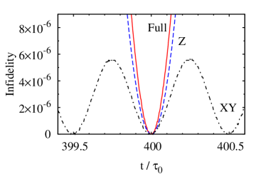
Figure 3: Simulated qubit infidelity $1-\langle F\rangle$ [Eq. (35)] in the vicinity of the first full rotation period of the double-dot qubit at $t=T$. Position-dependent magnetic field $B_{\mu}(\theta)$ is assumed static, and the rotation period $T$ is chosen commensurate with the Larmor frequency, $\omega_{0}T/2\pi=400$. Dashed line: only $B_{z}(\theta)$ is included; the infidelity minimum is exactly at $t=T$, in agreement with Eq. (54) which is exact in this situation. Dotted line: only the transverse components $B_{\mu}(\theta)$, $\mu=x,y$ are included. The infidelity minimum is slightly off the commensurate time $t=T$ due to the terms not included in Eq. (52). All three components of the field $B_{\mu}(\theta)$ are included for the red solid line.

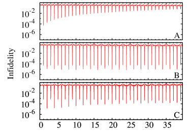
Figure 4: Simulation results for fidelity measured at the end of each cycle, for a linear time-dependence of $B_{1i}^{\mu}$ with (a) forward, (b) forward-back dot rotations [cf. Fig. 2], as well as (c) forward-back for quadratic time-dependence.

For the case of the static Overhauser field, see Fig. 3, we see that the average infidelity is dominated by the contribution from the $z$-component of the field, and that the infidelity nearly vanishes at the end of the spatial exchange protocol. For a linearly time-interpolated Overhauser field, the infidelity increases over several cycles of the single-direction $\pi$ pulses, Fig. 4a, but maintains a low value $\sim 10^{-5}$ after alternating between a sequence of two forward rotations, followed by two rotations in the opposite direction, Fig. 4b. However, for the quadratic interpolation, Fig. 4c, the infidelity gradually increases even for the alternating protocol, though it stays below $10^{-4}$ for several cycles.

VI Possible Experimental Setup

Aspects of our proposal, such as the precise construction of few-electron quantum dots in III-V semiconductor heterostructures have already been demonstrated in experiments. Petta et al. (2005); Reilly et al. (2008); van Weperen et al. (2011); Laird et al. (2010) However, the precise adiabatic rotation required in our proposal may be quite difficult to accomplish experimentally. We now discuss possible design implementations for an experimental realization, as well as physical constraints.

As discussed above, our proposal is suitable in materials with relatively weak spin-orbit coupling such as GaAs/AlGaAs heterostructures. We believe the electrons in a 2DEG could be confined in the radial direction by creating a circular depletion layer by placing electrostatic gates with a constant voltage in the center and outer edge of the circle as sketched in Figure 1. Since we wish to suppress the tunneling, the normal interdot spacing should be much larger than the dot size, $a$, so we assume that the circular trajectory has a radius $r_{0}\sim 15a\sim 1$ µm. Confinement and rotation in the angular direction could be accomplished by placing appropriately chosen time-dependent voltages on the ”wedge-gates” on both sides of the electron (Fig. 1). Several of these wedges will be needed to accomplish the smooth and adiabatic trajectory needed. The combined use of wedge and circular gates may require gates on both the top and bottom of the sample. The typical confining potential is approximated by $U\sim m\omega_{\text{d}}^{2}a^{2}$, which only requires reasonable gate voltages on the order of 100 mV.

The averaging of the hyperfine interaction is only valid in the quasi-static approximation of the Overhauser field. In general, the hyperfine interaction between the electron and the nuclei leads to a Knight shift. However, in the presence of the magnetic field, fluctuating corrections to the quasi-static approximation are inversely proportional to $B_{0}$ and can be neglectedTaylor et al. (2007). Thus, the most significant effect in this case is due to the dipole-dipole interaction of nearest neighboring nuclei which requires that $T\ll t_{\rm nuc}\sim 10^{-4}$sMerkulov et al. (2002). This places a lower bound on the velocity, while there is also an upper bound necessary to ensure that the Lorentz force from the dot rotation only deforms the actual path of the electron by a distance much smaller than the correlation length of the Overhauser field. This results in the restriction, $10^{-1}\ll v\ll 10^{5}$ in m/s. This rather lenient constraint is due to the assumption that confinement potential be large compared to the other potentials in our system. This allows us to neglect trajectory deviations from perturbations such as charge noise. In our estimates we also assumed $v$ to be small compared to the speed of sound, $s\sim 5\times 10^{3}$m/s. With $a/r_{0}\sim 15$ and $v\sim 10\,$m/s we obtain the rotation period $T\sim 1$ µs, which easily satisfies the above conditions and, according to our simulations, should result in the infidelities lower than $10^{-4}$ for significant time-scales. The rotation period could potentially be decreased to allow more operations to be performed before the states decohere.

VII Conclusion

We analyzed the real-space exchange of quantum dots as a possible substitute for the tunneling exchange. Ideally, exchange eliminates the hyperfine dephasing from the Overhauser field parallel to the applied field, leaving only the smaller effects from the in-plane field. The real-space exchange accomplishes the same suppression of the hyperfine interaction, but avoids the problematic sensitivity to charge noise present in exchange via tunneling. While spatial exchange does introduce additional effects such as spin-orbit coupling, simple tricks like using pairs of $\pi$ rotations in alternating directions can be used to suppress these so that the decoherence is still dominated by the hyperfine interaction. In particular, this field only enters as the small ratio of the average in-plane Overhauser field to the externally applied field. Perhaps the simplest way to suppress the hyperfine interaction in this approach is to reduce this ratio by increasing the externally applied field.

In addition, this spatial exchange is compatible with some of the methods already being attempted such as nuclear polarization via pumping. If the hyperfine interaction can be further suppressed, the next largest contribution from our spatial exchange approach would come from the disorder of the sample or the electron-phonon coupling. Our analysis of this spatial exchange also remains valid in systems that use additional quantum dots,Laird et al. (2010); van Weperen et al. (2011) with universal quantum operations in mind, as long as each operation is applied to only two dots at a time.

While the movement of quantum dots requires the precise control of the confining potential, which may be difficult to realize experimentally, our analysis shows that the construction of such a system is viable. With realistic parameter values from current experiments, our analysis produces infidelities smaller than $10^{-4}$ after ten decoupling cycles. This setup could also be a productive step towards the experimental realization of more complicated exchange systems, with many more interesting applications.

VIII Acknowledgements

This work was supported in part by the U.S. Army Research Office under Grant No. W911NF-11-1-0027 (LPP, DD), and by the NSF under Grants DMR-0748925 (KS, DD) and 1018935 (LPP, DD).

References

- Levy (2002) J. Levy, Phys. Rev. Lett., 89, 147902 (2002).
- Burkard et al. (1999) G. Burkard, D. Loss, and D. P. DiVincenzo, Phys. Rev. B, 59, 2070 (1999).
- Khaetskii et al. (2003) A. Khaetskii, D. Loss, and L. Glazman, Phys. Rev. B, 67, 195329 (2003).
- Gullans et al. (2010) M. Gullans, J. J. Krich, J. M. Taylor, H. Bluhm, B. I. Halperin, C. M. Marcus, M. Stopa, A. Yacoby, and M. D. Lukin, Phys. Rev. Lett., 104, 226807 (2010).
- Klauser et al. (2006) D. Klauser, W. A. Coish, and D. Loss, Phys. Rev. B, 73, 205302 (2006).
- Khodjasteh and Lidar (2005) K. Khodjasteh and D. A. Lidar, Phys. Rev. Lett., 95, 180501 (2005).
- Zhang et al. (2007) W. Zhang, V. V. Dobrovitski, L. F. Santos, L. Viola, and B. N. Harmon, Phys. Rev. B, 75, 201302 (2007).
- Imamoḡlu et al. (2003) A. Imamoḡlu, E. Knill, L. Tian, and P. Zoller, Phys. Rev. Lett., 91, 017402 (2003).
- Taylor et al. (2003) J. M. Taylor, C. M. Marcus, and M. D. Lukin, Phys. Rev. Lett., 90, 206803 (2003).
- Reilly et al. (2008) D. J. Reilly, J. M. Taylor, J. R. Petta, C. M. Marcus, M. P. Hanson, and A. C. Gossard, Science, 321, 817 (2008).
- Petta et al. (2005) J. R. Petta, A. C. Johnson, J. M. Taylor, E. A. Laird, A. Yacoby, M. D. Lukin, C. M. Marcus, M. P. Hanson, and A. C. Gossard, Science, 309, 2180 (2005).
- Barthel et al. (2010) C. Barthel, J. Medford, C. M. Marcus, M. P. Hanson, and A. C. Gossard, Phys. Rev. Lett., 105, 266808 (2010).
- van Weperen et al. (2011) I. van Weperen, B. D. Armstrong, E. A. Laird, J. Medford, C. M. Marcus, M. P. Hanson, and A. C. Gossard, Phys. Rev. Lett., 107, 030506 (2011).
- Golovach et al. (2010) V. N. Golovach, M. Borhani, and D. Loss, Phys. Rev. A, 81, 022315 (2010).
- Shitade et al. (2010) A. Shitade, M. Ezawa, and N. Nagaosa, Phys. Rev. B, 82, 195305 (2010).
- Silsbee (2004) R. H. Silsbee, Journal of Physics: Condensed Matter, 16, R179 (2004).
- Zawadzki and Pfeffer (2004) W. Zawadzki and P. Pfeffer, Semiconductor Science and Technology, 19, R1 (2004).
- Golovach et al. (2004) V. N. Golovach, A. Khaetskii, and D. Loss, Phys. Rev. Lett., 93, 016601 (2004).
- Krich and Halperin (2007) J. J. Krich and B. I. Halperin, Phys. Rev. Lett., 98, 226802 (2007).
- Pryadko and Quiroz (2009) L. P. Pryadko and G. Quiroz, Phys. Rev. A, 80, 042317 (2009).
- Pryadko and Sengupta (2006) L. P. Pryadko and P. Sengupta, Phys. Rev. B, 73, 085321 (2006).
- Uhrig (2007) G. S. Uhrig, Phys. Rev. Lett., 98, 100504 (2007).
- Laird et al. (2010) E. A. Laird, J. M. Taylor, D. P. DiVincenzo, C. M. Marcus, M. P. Hanson, and A. C. Gossard, Phys. Rev. B, 82, 075403 (2010).
- Taylor et al. (2007) J. M. Taylor, J. R. Petta, A. C. Johnson, A. Yacoby, C. M. Marcus, and M. D. Lukin, Phys. Rev. B, 76, 035315 (2007).
- Merkulov et al. (2002) I. A. Merkulov, Al. L. Efros, and M. Rosen, Phys. Rev. B, 65, 205309 (2002).