A class of pairwise models for epidemic dynamics on weighted networks

Abstract

In this paper, we study the $SIS$ (susceptible-infected-susceptible) and $SIR$ (susceptible-infected-removed) epidemic models on undirected, weighted networks by deriving pairwise-type approximate models coupled with individual-based network simulation. Two different types of theoretical/synthetic weighted network models are considered. Both models start from non-weighted networks with fixed topology followed by the allocation of link weights in either (i) random or (ii) fixed/deterministic way. The pairwise models are formulated for a general discrete distribution of weights, and these models are then used in conjunction with network simulation to evaluate the impact of different weight distributions on epidemic threshold and dynamics in general. For the $SIR$ dynamics, the basic reproductive ratio $R_{0}$ is computed, and we show that (i) for both network models $R_{0}$ is maximised if all weights are equal, and (ii) when the two models are equally matched, the networks with a random weight distribution give rise to a higher $R_{0}$ value. The models are also used to explore the agreement between the pairwise and simulation models for different parameter combinations.

Keywords: weighted network, pairwise model, moment closure

1 Introduction

Conventional models of epidemic spread consider a host population of identical individuals, each interacting in the same way with each of the others (see [2, 24, 45] and references therein). At the same time, in order to develop more realistic mathematical models for the spread of infectious diseases, it is important to obtain the best possible representation of the corresponding transmission mechanism. To achieve this, more recent models have included some of the many complexities that have been observed in mixing patterns. One such approach consists in splitting the population into a set of different subgroups, each with different social behaviours. Even more detail is included within network approaches, which allow to include differences between individuals, not just between sub-populations. In such models, each individual is represented as a node, and interactions that could permit the transmission of infection appear as edges linking nodes. The last decade has seen a substantial increase in the research of how infectious diseases are spread over large networks of connected nodes, where networks themselves can represent either small social contact networks or larger scale travel networks, including global aviation networks [22, 26, 37, 46, 52, 53, 54, 59, 60]. Importantly, the characteristics of the network, such as the average degree and the node degree distribution have a profound effect on the dynamics of the infectious disease spread, and hence significant efforts are made to capture properties of realistic contact networks.

Network models provide an intuitively appealing way to consider the social structure of populations, but they bring with them the challenge of collecting sufficient data to parameterise them fully. Ideally, an entire population would be sampled and all relevant interactions measured in order to reconstruct the contact network, but this is, unsurprisingly, seldom possible, and it is generally necessary to make suitable approximations. With the advance of computer-based tracking, statistical properties of many realistic networks (e.g. mobile phone calls) have been studied in great detail, and these are often used as proxy for the analysis of epidemic dynamics [26, 41].

One of the simplifying assumptions often put into models on networks is that all links are equally likely to transmit infection [14, 31, 46, 63]. However, a more detailed consideration leads to an observation that this is often not the case, as some links are likely to be far more capable of transmitting infection than others due to closer contacts (e.g. within households [11]) or long-duration interactions [18, 30, 62, 63, 64]. To account for this heterogeneity in properties of social interactions, network models can be adapted, thus resulting in weighted contact networks, where connections between different nodes have different weights. These weights may be associated with the duration, proximity, or social setting of the interaction, and the key point is that they are expected to be correlated with the risk of disease transmission. The precise relationship between the properties of an interaction and its riskiness is hugely complex; here, we will consider a“weight” that is exactly proportional to the transmission rate along a link. From a general perspective, one can consider two types of weighted networks: symmetric networks, where the strength only varies between different edges but is the same for a given pair of connected nodes, or go one step further and allow for the strength to be different even for the same pair of connected nodes $A$ and $B$, depending on whether $A$ infects $B$, or $B$ infects $A$. The first type of networks can be efficiently conceived as undirected graphs represented by symmetric connection matrices, while for the second one it is necessary to consider the contact network as a directed graph, resulting in a connection matrix, which in general is non-symmetric. Although consideration of weighted networks may seem as an additional complication for the analysis of epidemic dynamics, in fact it provides a much more realistic representation of actual contact networks.

Early models of weighted networks arose in the context of identifying genetic and metabolic networks [1, 56]. Later on, they found applications in a number of diverse research areas, such as international trade networks [10, 32], scientific collaboration networks [9, 33, 51], aviation networks of individual countries [3, 49] or global aviation networks [5, 20, 41] and networks of mobile phone communications [58]. Yook et al. [73] started a systematic study of evolving networks with nonbinary connectivities by considering growing weighted and exponential networks. This approach was later developed into a generic formalism for the analysis of evolving weighted networks [5, 6, 7, 50, 51]. Newman [55] has discussed general properties of weighted networks. Substantial amount of work has been done on the analysis of scale-free networks with different types of weight distribution [67, 74]. Wang et al. [68] have proposed a model with dynamical adjustment of weights in technological networks.

In epidemiological context, Yan et al. [70] analysed a model on weighted scale-free networks and found that heterogeneity in weight distribution leads to a slowdown in the spread of epidemics. Furthermore, they have shown that for a given network topology and mean infectivity, epidemics spread fastest in unweighted networks. Chu et al. [17] have investigated the dynamics of an $SI$ model on weighted scale-free networks with community structure and showed that the contribution coming from weights of edges connecting different communities exceeds the impact of weights on edges inside communities. Karsai et al. [43] have studied mean-field and finite-size scaling in weighted networks with small weights on edges connecting high-degree nodes. Yang et al. [72] have shown that disease prevalence can be maximized when the edge weights are chosen to be inversely proportional to the degrees of receiving nodes but, in this case, the transmissibility was not directly proportional to the weights and weights were also asymmetric. Yang & Zhou [71] have considered $SIS$ epidemics on homogeneous networks with uniform or power-law edge weight distribution and shown how to derive a certain type of mean-field description for such models. Britton et al. [15] have derived an expression for the basic reproductive ratio in weighted networks with generic distributions of node degree and weights, and Deijfen [23] has performed a similar analysis to study vaccination in such networks. In terms of practical epidemiological applications, weighted networks have already been effectively used to study control of global pandemics [19, 21, 29] and the spread of animal disease due to cattle movement between farms [35, 69]. Eames et al. [29] have considered an $SIR$ model on an undirected weighted network, where rather than using some theoretical formalism to generate an idealized network, the authors have relied on social mixing data obtained from questionnaires completed by members of a peer group [62] to construct a realistic weighted network. Having analysed the dynamics of epidemic spread in a such a network, they showed how information about node-specific infection risk can be used to develop targeted preventative vaccination strategies. As an alternative approach to modelling heterogeneity in network interactions, Eames [27] has considered a network with two types of contacts: random and regular, where the first type refers to arbitrary connections with any node in the network, while the second type designates multiple repeated contacts with the same nodes. He showed that in a highly clustered population, random contacts allow infection to reach otherwise inaccessible parts of the network, while in the case of all contacts being regular, clustering leads to a significant reduction in the spread of infection.

In this paper, we consider the dynamics of an infectious disease spreading on weighted networks with different weight distributions. Since we are primarily concerned with the effects of weight distribution on the disease dynamics, the connection matrix will be assumed to be symmetric, representing the situation when the weights can only be different for different network edges, but for a given edge the weight is the same irrespective of the direction of infection. From epidemiological perspective, we consider both the case when the disease confers permanent immunity (represented by an $SIR$ model), and the case when the immunity is short-lived, and upon recovery the individuals return to the class of susceptibles ($SIS$ model). For both of these cases we derive the corresponding ODE-based pairwise models and their closure approximations. Numerical simulation of both the network dynamics and the pairwise approximations are performed.

The outline of this paper is as follows. In the next section, the construction of specific weighted networks to be used for analysis of epidemic dynamics is discussed. This is complemented by the derivation of corresponding pairwise models and their closure approximations. Section 3 contains the derivation of the basic reproductive ratio $R_{0}$ for the $SIR$ model and for different weight distributions as well as numerical simulation of both network models and their pairwise ODE counterparts. The paper concludes in Section 4 with discussion of results and possible further extensions of this work.

2 Material and methods

2.1 Network construction

There are two conceptually different approaches to constructing weighted networks for modelling infectious disease spread. In the first approach, there is a seed or a primitive motif, and the network is then grown or evolved from this initial seed according to some specific rules. In this method, the topology of the network is co-evolving with the distribution of weights on the edges [6, 7, 8, 50, 72]. Another approach is to consider a weighted network as a superposition of an unweighted network with a distribution of weights across edges which could independent of the original network or it may be correlated with node metrics, such as their degree, [15, 23, 34, 66]. In this paper we use the second approach in order to investigate the particular role played by the distribution of weights across edges, rather than network topology, in the dynamics of epidemic spread. Besides computational efficiency, this will allow us to make some analytical headway in deriving and analysing low-dimensional pairwise models which are likely to perform better when weights are attached according to the scenarios described above.

Here we consider two different methods of assigning weights to network links: a network in which weights are assigned to links at random, and a network in which each node has the same distribution of weighted links connected to it. In reality, there is likely to be a great deal more structure to interaction weights, but in the absence of precise data and also for the purposes of developing models that allow one to explore a number of different assumptions, we make these simplifying approximations.

2.1.1 Random weight distribution

First we consider a simple model of an undirected weighted network with $N$ nodes where the weights of the links can take values $w_{i}$ with probability $p_{i}$, where $i=1,2,\dots,M$. The underlying degree distribution of the corresponding unweighted network can be chosen to be of the more basic forms, e.g. homogeneous random or Erdős-Rényi-type random networks.

The generation of such networks is straightforward, and weights can be assigned during link creation in the unweighted network. For example, upon using the configuration model for generating unweighted networks, each new link will have a weight assigned to it based on the chosen weight distribution. This means that in a homogeneous random network with each node having $k$ links, the distribution of link weights of different type will be multinomial, and it is given by

$$P(n_{w_{1}},n_{w_{2}},\dots,n_{w_{M}})=\frac{k!}{n_{w_{1}}!n_{w_{2}}!\dots n_{w_{M}}!}p_{1}^{n_{1}}p_{2}^{n_{2}}\dots p_{M}^{n_{M}},$$ (1)

where, $n_{w_{1}}+n_{w_{2}}+\cdots+n_{w_{M}}=k$ and $P(n_{w_{1}},n_{w_{2}},\dots,n_{w_{M}})$ stands for the probability of a node having $n_{w_{1}}$, $n_{w_{2}}$, $\dots$, $n_{w_{M}}$ links with weights $w_{1}$, $w_{2}$, $\dots$, $w_{M}$, respectively. While the above expression is applicable in the most general set-up, it is worth considering the case of weights of only two types, where the distribution of link weights for a homogenous random network becomes binomial

$$P(n_{w_{1}},n_{w_{2}}=k-n_{w_{1}})={k\choose n_{w_{1}}}p_{1}^{n_{1}}(1-p_{1})^{k-n_{1}},$$ (2)

where, $p_{1}+p_{2}=1$ and $n_{w_{1}}+n_{w_{2}}=k$. The average link weight in the model above can be easily found as

$$w_{av}^{random}=\sum_{i=1}^{M}p_{i}w_{i},$$

which for the case of weights of two types $w_{1}$ and $w_{2}$ reduces to

$$w_{av}^{(2r)}=p_{1}w_{1}+p_{2}w_{2}=p_{1}w_{1}+(1-p_{1})w_{2}.$$

2.1.2 Fixed deterministic weight distribution

As a second example we consider a network, in which each node has $k_{i}$ links with weight $w_{i}$ ($i=1,2,\dots,M$), where $k_{1}+k_{2}+\cdots+k_{M}=k$. The different weights here could be interpreted as being associated with different types of social interaction: e.g. home, workplace, and leisure contacts, or physical and non-physical interactions. In this model all individuals are identical in terms of their connections, not only having the same number of links (as in the model above) but also having the same set of weights. The average weight in such a model is given by

$$w_{av}^{fixed}=\sum_{i=1}^{M}p_{i}w_{i},\hskip 14.22636ptp_{i}=\frac{k_{i}}{k},$$

where $p_{i}$ is the fraction of links of type $i$ for each node. In the case of links of two types with weights $w_{1}$ and $w_{2}$, the average weight becomes

$$w_{av}^{(2f)}=p_{1}w_{1}+p_{2}w_{2}=\frac{k_{1}}{k}w_{1}+\frac{k_{2}}{k}w_{2}=\frac{k_{1}}{k}w_{1}+\frac{k-k_{1}}{k}w_{2}.$$

2.1.3 Epidemic models

In this study, the simple $SIS$ and $SIR$ epidemic models are considered. The epidemic dynamics is specified in terms of infection and recovery events. The rate of transmission across an unweighted edge between an infected and susceptible individual is denoted by $\tau$. This will then be adjusted by the weight of the link which is assumed to be directly proportional to the strength of the transmission along that link. Infected individuals recover independently of each other at rate $\gamma$. The simulation is implemented using Gillespie algorithm [36] with inter-event times distributed exponentially with a rate given by the total rate of change in the network, with the single event to be implemented at each step being chosen at random and proportionally to its rate. All simulations start with most nodes being susceptible and with a few infected nodes chosen at random.

2.2 Pairwise equations

In this section we extend the classic pairwise model for unweighted networks [44, 61] to the case of weighted graphs with $M$ different link-weight types. Pairwise models successfully interpolate between classic compartmental ODE models and full individual-based network simulation with the added advantage of high transparency and a good degree of analytical tractability. These qualities makes them an ideal tool for studying dynamical processes on networks [27, 38, 40, 44], and they can be used on their own and/or in parallel with simulation. The original versions of the pairwise models have been successfully extended to networks with heterogenous degree distribution [28], asymmetric networks [65] and situations where transmission happens across different/combined routes [27, 38] as well as when taking into consideration network motifs of higher order than pairs and triangles [39]. The extension that we propose is based on the previously established precise counting procedure at the level of individuals, pairs and triples, as well as on a careful and systematic account of all possible transitions needed to derive the full set of evolution equations for singles and pairs. These obviously involve the precise dependency of lower order moments on higher order ones, e.g. the rate of change of the expected number of susceptible nodes is proportional to the expected number of links between a susceptible and infected node. We extend the previously well-established notation [44] to account for the added level of complexity due to different link weights. In line with this, the number of singles remains unchanged, with $[A]$ denoting the number of nodes across the whole network in state $A$. Pairs of type $A-B$, $[AB]$, are now broken down depending on link weights, i.e. $[AB]_{i}$ represents the number of links of type $A-B$ with the link having weight $w_{i}$, where as before $i=1,2,\dots,M$ and $A,B\in\{S,I,R\}$ if an $SIR$ dynamics is used. As before, links are doubly counted (e.g. in both directions) and thus the following relations hold: $[AB]_{m}=[BA]_{m}$ and $[AA]_{m}$ is equal to twice the number of uniquely counted links of weight $w_{m}$ with nodes at both ends in state $A$. From this extension it follows that $\sum_{i=1}^{M}[AB]_{i}=[AB]$. The same convention holds at the level of triples where $[ABC]_{mn}$ stands for the expected number of triples where a node in state $B$ connects a node in state $A$ and $C$ via links of weight $w_{m}$ and $w_{n}$, respectively. The weight of the link impacts on the rate of transmission across that link, and this is achieved by using a link-specific transmission rate equal to $\tau w_{i}$, where $i=1,2,\dots,M$. In line with the above, we construct two pairwise models, one for $SIS$ and one for $SIR$ dynamics.

The pairwise model for the $SIS$ dynamics can be written in the form:

$$\begin{array}[]{l}[\dot{S}]=\gamma{[I]}-\tau{\sum_{n=1}^{M}{w_{n}}{[SI]_{n}}},\\ \\ \ [\dot{I}]=\tau{\sum_{n=1}^{M}{w_{n}}{[SI]_{n}}}-\gamma{[I]},\\ \\ \ [\dot{SI}]_{m}=\gamma{([II]_{m}-[SI]_{m})}+\tau{\sum_{n=1}^{M}{w_{n}}{([SSI]_{mn}-[ISI]_{nm})}}-\tau{w_{m}}{[SI]_{m}},\\ \\ \ [\dot{II}]_{m}=-2{\gamma{[II]_{m}}}+2{\tau}{\sum_{n=1}^{M}w_{n}{[ISI]_{nm}}}+2{\tau}{w_{m}}{[SI]_{m}},\\ \\ \ [\dot{SS}]_{m}=2{\gamma{[SI]_{m}}}-2{\tau{\sum_{n=1}^{M}w_{n}{[SSI]_{mn}}}},\end{array}$$ (3)

where $m=1,2,3,...,M$ and $[AB]_{m}$ denotes the expected number of links with weight $w_{m}$ connecting two nodes of type $A$ and $B$, respectively ($A,B\in\{S,I\}$).

In the case when upon infection individuals recover at rate $\gamma$ and once recovered they maintain a life-long immunity, we have the following system of equations describing the dynamics of a pairwise $SIR$ model:

$$\begin{array}[]{l}\dot{[S]}=-\tau{\sum_{n=1}^{M}{w_{n}}{[SI]_{n}}},\\ \\ \dot{[I]}=\tau{\sum_{n=1}^{M}{w_{n}}{[SI]_{n}}}-\gamma{[I]},\\ \\ \dot{[R]}=\gamma{[I]},\\ \\ \ [\dot{S}{S}]_{m}=-2{\tau{\sum_{n=1}^{M}{w_{n}}{[SSI]_{mn}}}},\\ \\ \ [\dot{S}{I}]_{m}=\tau{\sum_{n=1}^{M}{w_{n}}{([SSI]_{mn}-[ISI]_{nm})}}-\tau{w_{m}}{[SI]_{m}}-\gamma{[SI]_{m}},\\ \\ \ [\dot{S}{R}]_{m}=-{\tau{\sum_{n=1}^{M}{w_{n}}{[ISR]_{nm}}}}+\gamma{[SI]_{m}},\\ \\ \ [\dot{I}{I}]_{m}=2{\tau}{\sum_{n=1}^{M}w_{n}{[ISI]_{nm}}}+2{\tau}{w_{m}{[SI]_{m}}}-2{\gamma}{[II]_{m}},\\ \\ \ [\dot{I}{R}]_{m}={\tau{\sum_{n=1}^{M}{w_{n}}{[ISR]_{nm}}}}+\gamma{([II]_{m}-[IR]_{m})},\\ \\ \ [\dot{R}{R}]_{m}=\gamma{[IR]_{m}},\end{array}$$ (4)

where again $m=1,2,3,...,M$ with the same notation as above.

The above systems of equations (3) and (4) are not closed, as equations for the pairs require knowledge of triples, and thus, equations for triples are needed. This dependency on higher-order moments can be curtailed by closing the equations via approximating triples in terms of singles and pairs [44]. For both systems, the agreement with simulation will heavily depend on the precise distribution of weights across the links, the network topology, and the type of closures that will be used to capture essential features of network structure and the weight distribution. As a check and a reference back to previous model, in Appendix A shows how systems (3) and (4) reduce to the standard unweighted pairwise $SIS$ and $SIR$ models [44] when all weights are equal to each other, $w_{1}=w_{2}=\cdots=w_{M}=W$.

2.2.1 Closure relations

The most natural extension of the classic closure is given by

$$[ABC]_{mn}=\frac{k-1}{k}\frac{[AB]_{m}[BC]_{n}}{[B]},$$ (5)

where $k$ is the number of links per node for a homogeneous natwork or the average nodal degree for networks with other than homogenous degree distributions. Even for the simplest case of homogenous random networks with two weights, a different version of the closure can be derived. The starting point for this different closure is the observation that the average number of links of weight $w_{1}$ across the whole network is $k_{1}=p_{1}k\leq k$, and similarly, the average number of links of weight $w_{2}$ is $k_{2}=(1-p_{1})k\leq k$. This motivates the following closures

$$\begin{array}[]{l}\displaystyle{\ [ABC]_{11}=[AB]_{1}(k_{1}-1)\frac{[BC]_{1}}{k_{1}[B]}=\frac{k_{1}-1}{k_{1}}\frac{[AB]_{1}[BC]_{1}}{[B]},}\\ \\ \displaystyle{\ [ABC]_{12}=[AB]_{1}k_{2}\frac{[BC]_{2}}{k_{2}[B]}=\frac{[AB]_{1}[BC]_{2}}{[B]},}\\ \\ \displaystyle{\ [ABC]_{21}=[AB]_{2}k_{1}\frac{[BC]_{1}}{k_{1}[B]}=\frac{[AB]_{2}[BC]_{1}}{[B]},}\\ \\ \displaystyle{\ [ABC]_{22}=[AB]_{2}(k_{2}-1)\frac{[BC]_{2}}{k_{2}[B]}=\frac{k_{2}-1}{k_{2}}\frac{[AB]_{2}[BC]_{2}}{[B]}.}\end{array}$$ (6)

The specific choice of closure will depend on the structure of the network and, especially, how the weights are distributed. For example, for the case of the homogeneous random networks with links allocate randomly, both closures offer a viable alternative. For the case of a network where each node has a fixed pre-allocated number of links with different weights, e.g. $k_{1}$ and $k_{2}$ links with weights $w_{1}$ and $w_{2}$, respectively, the second closure (6) offers the more natural/intuitive avenue towards closing the system and obtaining good agreement with network simulation.

3 Results

In this section we present analytical and numerical results for weighted networks and pairwise representations of $SIS$ and $SIR$ models in the case of two different link-weight types (i.e. $w_{1}$ and $w_{2}$).

3.1 Threshold dynamics for the $SIR$ model - the network perspective

The basic reproductive ratio, $R_{0}$ (the average number of secondary cases produced by a typical index case in an otherwise susceptible population), is one of the most fundamental quantities in epidemiology ([2, 25]). Besides informing us on whether a particular disease will spread in a population, as well as quantifying the severity of an epidemic outbreak, it can be also used to calculate a number of other important quantities that have good intuitive interpretation. In what follows, we will compute $R_{0}$ and $R_{0}$-like quantities and will discuss their relation to each other, and also issues around these being model-dependent. First, we compute $R_{0}$ from an individual-based or network perspective by employing the next generation matrix approach as used in the context of models with multiple transmission routes such as household models [4].

Random weight distribution: First we derive an expression for $R_{0}$ when the underlying network is homogeneous, and the weights of the links are assigned at random according to a prescribed weight distribution. In the spirit of the proposed approach, the next generation matrix can be easily computed to yield

$$NGM=(a_{ij})_{i,j=1,2}=\left|\begin{array}[]{cc}(k-1)p_{1}r_{1}&(k-1)p_{1}r_{1}\\ (k-1)p_{2}r_{2}&(k-1)p_{2}r_{2}\end{array}\right|,$$

where

$$r_{1}=\frac{\tau w_{1}}{\tau w_{1}+\gamma},\hskip 14.22636ptr_{2}=\frac{\tau w_{2}}{\tau w_{2}+\gamma}$$

represent the probability of transmission from an infected to a susceptible across a link of weight $w_{1}$ and $w_{2}$, respectively. Here, the entry $a_{ij}$ stands for the average number of infections produced via links of type $i$ (i.e. with weight $w_{i}$) by a typical infectious node who itself has been infected across a link of type $j$ (i.e. with weight $w_{j}$). Using the fact that $p_{2}=1-p_{1}$, the basic reproductive ratio can be found from the leading eigenvalue of the $NGM$ matrix as follows

$$R_{0}^{1}=(k-1)(p_{1}r_{1}+(1-p_{1})r_{2}).$$ (7)

In fact, the expression for $R_{0}$ can be simply generalised to more than two weights to give $R_{0}=(k-1)\sum_{i=1}^{M}p_{i}r_{i}$, where $w_{m}$ has frequency given by $p_{m}$ with the constraint that $\sum_{i=1}^{M}p_{i}=1$. It is straightforward to show that upon assuming uniform weight distribution $w_{i}=W$ for $i=1,2,\dots,M$, the basic reproduction number on a homogeneous graph reduces to $R_{0}=(k-1)r$ as expected, and where, $r=\tau W/(\tau W+\gamma)$.

Deterministic weight distribution: The case when the number of links with given weights for each node is fixed can be captured with the same approach, and the next generation matrix can be constructed as follows

$$NGM=\left|\begin{array}[]{cc}(k_{1}-1)r_{1}&k_{1}r_{1}\\ k_{2}r_{2}&(k_{2}-1)r_{2}\end{array}\right|.$$

As before, the leading eigenvalue of the $NGM$ matrix yields the basic reproductive ratio,

$$R_{0}^{2}=\frac{(k_{1}-1)r_{1}+(k_{2}-1)r_{2}+\sqrt{[(k_{1}-1)r_{1}-(k_{2}-1)r_{2}]^{2}+4k_{1}k_{2}r_{1}r_{2}}}{2}.$$ (8)

Using these two equivalent expressions for the basic reproductive ratio, it is possible to prove the following result.

Theorem 1. Given the setup for the fixed weight distribution and using $p_{1}=k_{1}/k$, $p_{2}=k_{2}/k$ and $k_{1}+k_{2}=k$, if $1\leq k_{1}\leq k-1$ (which implies that $1\leq k_{2}\leq k-1$), then $R_{0}^{2}\leq R_{0}^{1}$.

The proof of this result is sketched out in Appendix B. This Theorem effectively states that provided each node has at least one link of type 1 and one link of type 2, then independently of disease parameters, it follows that the basic reproductive ratio as computed from (7) always exceeds or is equal to an equivalent $R_{0}$ computed from (8).

It is worth noting that both $R_{0}$ values reduce to

$$R_{0}^{1}=R_{0}^{2}=R_{0}=(k-1)r=\frac{(k-1)\tau W}{\tau W+\gamma},$$ (9)

if one assumes that weights are equal, i.e. $w_{1}=w_{2}=W$. As one would expect, the first good indicator of the impact of weights on the epidemic dynamics will be the average weight. Hence, it is worth considering the problem of maximising the values $R_{0}$ under assumption of a fixed average weight:

$$p_{1}w_{1}+p_{2}w_{2}=W.$$ (10)

Under this constraint the following statement holds.

Theorem 2. For weights constrained by $p_{1}w_{1}+p_{2}w_{2}=W$ (or $(k_{1}/k)w_{1}+(k_{2}/k)w_{2}=W$ for a fixed weights distribution), $R_{0}^{1}$ and $R_{0}^{2}$ attain their maxima when $w_{1}=w_{2}=W$, and the maximum values for both is $\displaystyle{R_{0}=(k-1)r=\frac{(k-1)\tau W}{\tau W+\gamma}}$.

The proof of this result is presented in Appendix C.

The above results suggest that for the same average link weight and when the one-to-one correspondence between $p_{1}$ and $k_{1}/k$, and $p_{2}$ and $k_{2}/k$ holds, the basic reproductive ratio is higher on networks with random weight distribution than on networks with a fixed weight distribution. This, however, does not preclude the possibility of having a network with random weight distribution with smaller average weight exhibiting an $R_{0}$ value that it is bigger than the $R_{0}$ value corresponding to a network where weights are fixed and the average weight is higher. The direct implication is that it is not sufficient to know just the average link weight in order to draw conclusions about possible epidemic outbreaks on weighted networks; rather one has to know the precise weight distribution that provides a given average weight.

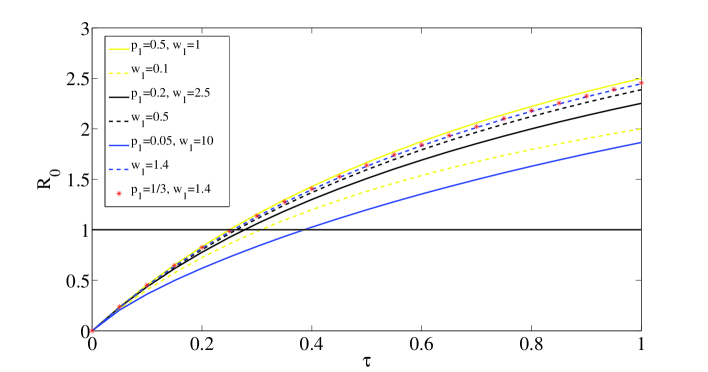
Figure 1: Plots of the basic reproductive ratio $R_{0}$ for the two types of weighted networks with different weight and weight frequency combinations, but with $p_{1}w_{1}+p_{2}w_{2}=1$. The case of homogenous networks with weights assigned at random (continuous lines with $p_{1}$ and $w_{1}$ given in the legend) considers the situation where the contribution of the two different weight types is equal ($p_{1}w_{1}=p_{2}w_{2}=0.5$) but with weight $w_{1}$ increasing (top to bottom) and its frequency decreasing. Increasing the magnitude of weights but reducing their frequency leads to smaller $R_{0}$ values. The case of homogeneous networks with fixed number of links of type $w_{1}$ and $w_{2}$ (dashed lines with only $w_{1}$ given in the legend) illustrates the situation where $w_{1}$ increases (bottom to top) while $p_{1}=k_{1}/k=1/3$ and $p_{2}=(k-k_{1})/k=2/3$ remain fixed. Here the opposite tendency is observed with increasing weights leading to higher $R_{0}$ values. Finally, for the randomly distributed weights case, setting $p_{1}=1/3,w_{1}=1.4$ and observing $p_{1}w_{1}+p_{2}w_{2}=1$, we obtain $R_{0}$ ($\star$) values which compare almost directly to the fixed-weights case (top, dashed line). Other parameters are set to $k=6$, $k_{1}=2$ and $\gamma=1$.

Figure 1 shows how the basic reproductive ratio changes with the transmission rate $\tau$ for different weight distributions. When links on a homogeneous network are distributed at random, the increase in the magnitude of one specific link weight (e.g. $w_{1}$) accompanied by a decrease in its frequency leads to smaller $R_{0}$ values. This is to be expected since the contribution of the different link types in this case is kept constant ($p_{1}w_{1}=p_{2}w_{2}=0.5$) and this implies that the overall weight of the network links accumulates in a small number of highly weighted links with most links displaying small weights and thus making transmission less likely. The statement above is more rigorously underpinned by the results of Theorem 1 & 2 which clearly show that equal or more homogeneous weights lead to higher values of the basic reproductive ratio. For the case of fixed weight distribution, the changes in the value of $R_{0}$ are investigated in terms of varying the weights, so that overall weight in the network remains constant. This is constrained by fixing values of $p_{1}$ and $p_{2}$ and, in this case, the highest values are obtained for higher values of $w_{1}$. The flexibility here is reduced due to $p_{1}$ and $p_{2}$ being fixed, and a different link breakdown may lead to different observations. The top continuous line in Fig. 1 corresponds to the maximum $R_{0}$ value achievable for both models if the $p_{1}w_{1}+p_{2}w_{2}=1$ constraint is fulfilled.

3.2 $R_{0}$-like threshold for the $SIR$ model - a pairwise model perspective

To compute the value of $R_{0}$-like quantity from the pairwise model, we use the approach suggested by Keeling [44], which utilises the local spatial/network structure and correctly accounts for correlations between susceptible and infectious nodes early on in the epidemics. This can be achieved by looking at the early behaviour of $[SI]_{1}/[I]=\lambda_{1}$ and $[SI]_{2}/[I]=\lambda_{2}$ when considering links of only two different weights. In line with Eames [27], we start from the evolution equation of $[I]$

$$\dot{[I]}=(\tau w_{1}[SI]_{1}/[I]+\tau w_{2}[SI]_{2}/[I]-\gamma)[I],$$

where from the growth rate $\tau w_{1}\lambda_{1}+\tau w_{2}\lambda_{2}-\gamma$ it is easy to define the threshold quantity $R$ as follows,

$$R=\frac{\tau w_{1}\lambda_{1}+\tau w_{2}\lambda_{2}}{\gamma}.$$ (11)

For the classic closure (5), one can compute the early quasi-equilibria for $\lambda_{1}$ and $\lambda_{2}$ directly from the pairwise equations as follows

$$\lambda_{1}=\frac{\gamma{(k-1)}{p_{1}}{R}}{\tau{w_{1}}+\gamma{R}}\,\,\,\text{and}\,\,\,\lambda_{2}=\frac{\gamma{(k-1)}(1-p_{1}){R}}{\tau{w_{2}}+\gamma{R}}.$$

Substituting these into (11) and solving for $R$ yields

$$R=\frac{R_{1}+R_{2}+\sqrt{(R_{1}+R_{2})^{2}+4R_{1}R_{2}Q}}{2},$$ (12)

where

$$\begin{array}[]{l}\displaystyle{R_{1}=\frac{\tau{w_{1}}[(k-1)p_{1}-1]}{\gamma},\hskip 8.5359ptR_{2}=\frac{\tau{w_{2}}[(k-1)p_{2}-1]}{\gamma},}\\ \\ \displaystyle{Q=\frac{k-2}{[(k-1)p_{1}-1][(k-1)p_{2}-1]},}\end{array}$$

with details of all calculations presented in Appendix D. We note that $R>1$ will result in an epidemic, while $R<1$ will lead to the extinction of the disease. It is straightforward to show that for equal weights, say $W$, the expression above reduces to $R=\tau W(k-2)/\gamma$ which is in line with $R_{0}$ value in [44] for unclustered, homogeneous networks. Under the assumption of a fixed total weight $W$, one can show that similarly to the network-based basic reproductive ratio, $R$ achieves its maximum when $w_{1}=w_{2}=W$.

In a similar way, for the modified closure (6), we can use the same methodology to derive the threshold quantity as

$$R=\frac{R_{1}+R_{2}+\sqrt{(R_{1}+R_{2})^{2}+4R_{1}R_{2}(Q-1)}}{2},$$ (13)

where

$${R_{1}=\frac{\tau{w_{1}}(k_{1}-2)}{\gamma},\hskip 8.5359ptR_{2}=\frac{\tau{w_{2}}(k_{2}-2)}{\gamma},\hskip 8.5359ptQ=\frac{k_{1}k_{2}}{(k_{1}-2)(k_{2}-2)}.}$$

For this closure once again, $R>1$ results in an epidemic, while for $R<1$, the disease dies out. Details of this calculations are shown in Appendix D. It is noteworthy that one can derive expressions (12) and (13) by considering the leading eigenvalue of linearization of system (4) near its disease-free steady state with the corresponding pairwise closures given in (5) and (6).

Finally, we note that this seemingly $R_{0}$-lookalike, $R=\tau W(k-2)/\gamma$ for the equal weights case $w_{1}=w_{2}=W$ is a multiple of $(k-2)$ as opposed to $(k-1)$ as is the case for the $R_{0}$ derived based on the individual-based perspective, where, for equal weights, $R_{0}^{1}=R_{0}^{2}=\tau W(k-1)/(\tau W+\gamma)$. This obviously highlights the strong dependency of $R_{0}$ on the modelling framework and also the difficulty in trying to reconcile findings based on different models.

3.3 The performance of pairwise models and the impact of weight distributions on the dynamics of epidemics

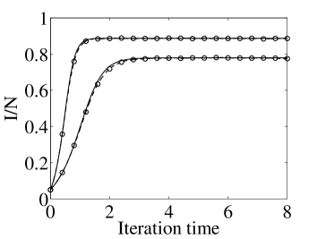
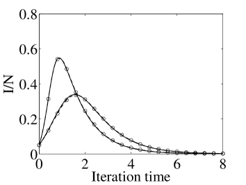
Figure 2: The infection prevalence ($I/N$) from the pairwise and simulation models for homogeneous random networks with random weight distribution (ODE: solid line, simulation: dashed line and (o)). All nodes have degree $k=5$ with $N=1000$, $I_{0}=0.05N$, $\gamma=1$ and $\tau=1$. From top to bottom, the parameter values are: $w_{1}=5,p_{1}=0.2,w_{2}=1.25,p_{2}=0.8$ (top), and $w_{1}=0.5,p_{1}=0.5,w_{2}=1.5,p_{2}=0.5$ (bottom). The left and right panels represent the $SIS$ and $SIR$ dynamics, respectively.

To evaluate the efficiency of the pairwise approximation models, we will now compare numerical solutions of models (3) and (4) to results obtained from the corresponding network simulation. The discussion around the comparison of the two models is interlinked with the discussion of the impact of different weight distributions/patterns on the overall epidemic dynamics. We being our numerical investigation by considering weight distributions with moderate heterogeneity. This is illustrated in Fig. 2, where excellent agreement between simulation and pairwise models is obtained. The agreement remains valid for both $SIS$ and $SIR$ dynamics, and networks with higher average link weight lead to higher prevalence levels at equilibrium for $SIS$ and higher infectiousness peaks for $SIR$.

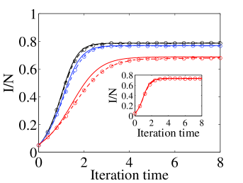
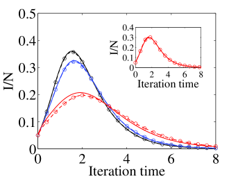
Figure 3: The infection prevalence ($I/N$) from the pairwise and simulation models for homogenous networks with random weight distribution (ODE: solid line, simulation: dashed line and (o)). All numerical tests use $N=1000$, $I_{0}=0.05N$, $k=5$, $\gamma=1,\tau=1$ and $p_{1}=0.05$ ($p_{2}=1-p_{1}=0.95$). From top to bottom, $w_{1}=2.5,5,10$, $w_{2}=0.875/0.95,0.75/0.95,0.5/0.95$. The weight distributions are chosen such that the average link weight, $p_{1}w_{1}+p_{2}w_{2}=1$, remains constant. Insets of (a) and (b): the same parameter values as for the lowest prevalence plots but, with $k=10$ and $\tau=0.5$. The left and right panel represent the $SIS$ and $SIR$ dynamics, respectively.

Next, we explore the impact of weight distribution under the condition that the average weight remains constant (i.e. $p_{1}w_{1}+p_{2}w_{2}=1$, where without loss of generality the average weight has been chosen to be equal to 1). First, we keep the proportion of edges of type one (i.e. with weight $w_{1}$) fixed and change the weight itself by gradually increasing its magnitude. Due to the constraint on the average weight and the condition $p_{2}=1-p_{1}$, the other descriptors of the weight distribution follow. Fig. 3 shows that concentrating a large portion of the total weight on a few links leads to smaller epidemics, since the majority of links are low-weight and thus have a small potential to transmit the disease. This effect is exacerbated for the highest value of $w_{1}$; in this case $95\%$ of the links are of weight $w_{2}=(1-p_{1}w_{1})/(1-p_{1})=0.5/0.95$ leading to epidemics of smallest impact (Fig. 3(a)) and smallest size of outbreak (Fig. 3(b)).

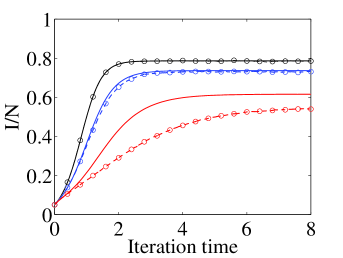
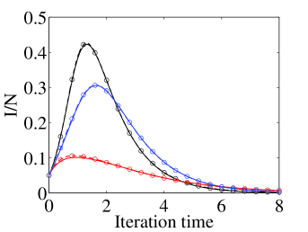
Figure 4: The infection prevalence ($I/N$) from the pairwise and simulation model for homogenous networks with random weight distribution (ODE: solid line, simulation: dashed line and (o)). All numerical tests use $N=1000$, $I_{0}=0.05N$, $k=10$, $\gamma=1,\tau=0.5$ and $w_{1}=10$. From top to bottom, $P(w_{1})=0.01,0.05,0.09$, $w_{2}=0.9/0.99,0.5/0.95,0.1/0.91$. Here also $p_{2}=1-p_{1}$ and $p_{1}w_{1}+p_{2}w_{2}=1$. The left and right panel represent the $SIS$ and $SIR$ dynamics, respectively.

While the previous setup kept the frequency of links constant while changing the weights, one can also investigate the impact of keeping at least one of the weights constant (e.g. the larger one) and changing its frequency. To ensure a fair comparison, here we also require that the average link weight over the whole network is kept constant. When such highly weighted links are rare, the system approaches the non-weighted network limit where the transmission rate is simply scaled by $w_{2}$ (the most abundant link type). As Fig. 4 shows, in this case, the agreement is excellent, and as the frequency of the highly weighted edges/links increases, disease transmission is less severe.

Regarding the comparison of the pairwise and simulation models, we note that while the agreement is generally good for a large part of the disease and weight parameter space, the more extreme scenarios of weight distribution result in poorer agreement. This is illustrated in both Figs. 3 and 4 (see bottom curves), with the worst agreement for the $SIS$ dynamics. The insets in Fig. 3 show that increasing the average connectivity improves the agreement. However, the cause of disagreement is due to a more subtle effect driven also by the weight distribution. For example, in Fig. 4, the average degree in the network is $10$, higher then used previously and equal to that in the insets from Fig. 3, but despite this, the agreement is still poor.

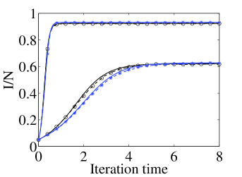
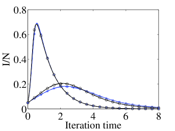
Figure 5: The infection prevalence ($I/N$) based on random (model 1) and fixed (model 2) weight distribution (ODE: black (1) and blue (2) solid line, simulation results: same as ODE but dashed lines, and ($\circ$) and ($\ast$)). All numerical tests use $N=1000$, $I_{0}=0.05N$, $k=10$, $k_{1}=2$, $k_{2}=8$, $p_{1}=k_{1}/k$, $p_{2}=k_{2}/k$, $w_{1}=10$, $w_{2}=1.25$ and $\gamma=1$. The rate of infection $\tau=0.5$ (top) and $\tau=0.1$ (bottom). The left and right panel represent the $SIS$ and $SIR$ dynamics, respectively.

The two different weighted network models are compared in Fig. 5. This is done be using the same link weights and setting $p_{1}=k_{1}/k$ and $p_{2}=k_{2}/k$. Epidemics on network with random weight distribution grow faster and, given the same time scales of the epidemic, this is line with results derived in Theorem 1 & 2 and findings concerning the growth rates. The difference is less marked for larger values of $\tau$ where a significant proportion of the nodes becomes infected.

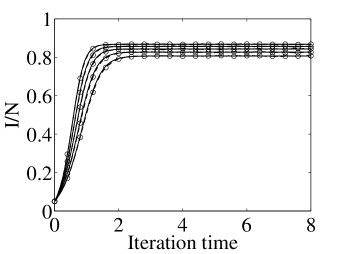
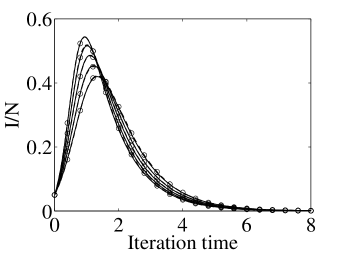
Figure 6: The infection prevalence ($I/N$) for a fixed weight distribution (ODE: solid lines, simulation results: dashed lines and (o)). All numerical tests use $N=1000$, $I_{0}=0.05N$, $k=6$, $\gamma=1,\tau=1$ and $w_{1}=1.4,w_{2}=0.8$. From top to bottom : $k_{1}=5,4,3,2,1$ and $k_{2}=k-k_{1}$. The left and right panel represent the $SIS$ and $SIR$ dynamics, respectively.

In Fig. 6 the link weight composition is altered by decreasing the proportion of highly-weighted links. As expected, the reduced average link weight across the network leads to epidemics of smaller size while keeping the excellent agreement between simulation and pairwise model results.

4 Discussion

The present study has explored the impact of weight heterogeneity and highlighted that the added heterogeneity of link weights does not manifest itself in the same way as most other heterogeneities in epidemic models on networks. Usually, heterogeneities lead to an increase in $R_{0}$ but potentially for final size to fall. However, for weighted networks the concentration of infectiousness on fewer target link, and thus target individuals, leads to a fall in $R_{0}$ for both homogeneous random and fixed weight distribution models. Increased heterogeneity in weights accentuates the locality of contact and is taking the model further from the mass-action type models. Infection is concentrated along a smaller number of links, which results in wasted infectivity and lower $R_{0}$. This is in line with similar results [15, 16, 70] where different modelling approaches have been used to capture epidemics on weighted networks.

The models proposed in this paper are simple mechanistic models with basic weight distributions, but despite this they provide a good basis for analysing disease dynamics on weighted networks in a rigorous and systematic way. The modified pairwise models have performed well, and provide good approximation to direct simulation. As expected, the agreement with simulations typically breaks down at or close to the threshold, but away from it, pairwise models provide a good counterpart or alternative to simulation. Disagreement only appears for extreme weight distributions, and we hypothesise that this is mainly due to the network becoming more modular with islands of nodes connected by links of low weight being bridged together by highly weighted links. A good analogy to this is provided by considering the case of a pairwise model on unweighted networks specified in terms of two network metrics, node number $N$ and average number of links $k$. The validity of the pairwise model relies on the network being connected up at random, or according to the configuration model. This can be easily broken by creating two sub-networks of equal size both exhibiting the same average connectivity. Simulations on such type of networks will not agree with the pairwise model, and highlights that the network generating algorithm can push the network out of the set of ‘acceptable’ networks. We expect that this or similar argument can more precisely explain why the agreement breaks down for significant link-weight heterogeneity.

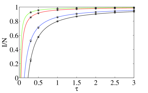
Figure 7: Endemic steady state from the $SIS$ model on networks with random weight distribution. The continuous lines correspond to the steady state computed numerically by setting all evolution equations in the pairwise system to zero. These are complemented by finding the endemic steady state through direct integration of the ODE system for a long-enough time ($\circ$), as well as direct simulation ($\ast$). The first marker corresponds to $\tau=0.3$ followed by $\tau=0.5,1.0,\dots,3.0$. All results are based on: $k=5$, $\gamma=1$ and $w_{1}=10,w_{2}=1$. From top to bottom : $p_{1}=0.9,0.5,0.1,0.01$ and $p_{2}=1-p_{1}$.

The usefulness of pairwise models is illustrated in Fig. 7, where the $I/N$ values are plotted for a range of $\tau$ values and for different weight distributions. Here, the equilibrium value has been computed by finding the steady state directly from the ODEs (3) by finding numerically the steady state solution of a set on nonlinear equations (i.e. $\dot{[A]}=0$ and $\dot{[AB]}=0$). To test the validity, the long term solution of the ODE is plotted along with results based on simulation. The agreement away from the threshold is excellent and illustrates clearly the impact of different weight distributions on the magnitude of the endemic threshold.

The models proposed here can be extended in a number of different ways. One potential avenue for further research is the analysis of correlations between link weight and node degree. This direction has been explored but in the context of classic compartmental mean-field models based on node degree [42, 57]. Given that pairwise models extend to heterogeneous networks such avenues can be further explored to include different type of correlations or other network dependent weight distributions. While this is a viable direction, it is expected that the extra complexity will make the pairwise models more difficult to analyse and disagreement between pairwise and simulation model more likely. Another theoretically interesting and practically important aspect is the consideration of different types of time delays, representing latency or temporary immunity [13], and the analysis of their effects on the dynamics of epidemics on weighted networks. The methodology presented in this paper can be of wider relevance to studies of other natural phenomena where overlay networks provide effective description. Examples of such systems include the simultaneous spread of two different diseases in the same population [12], the spread of the same disease but via different routes [47] or the spread of epidemics concurrently with information about the disease [38, 48]. These areas offer other important avenues for further extensions.

5 Appendix

5.1 Appendix A - Reducing the weighted pairwise models to the unweighted equivalents

We start from the system

$$\begin{array}[]{l}\dot{[S]}=\gamma{[I]}-\tau{\sum_{n=1}^{M}{w_{n}}{[SI]_{n}}},\\ \\ \dot{[I]}=\tau{\sum_{n=1}^{M}{w_{n}}{[SI]_{n}}}-\gamma{[I]},\\ \\ \ [\dot{SI}]_{m}=\gamma{([II]_{m}-[SI]_{m})}+\tau{\sum_{n=1}^{M}{w_{n}}{([SSI]_{mn}-[ISI]_{nm})}}-\tau{w_{m}}{[SI]_{m}},\\ \\ \ [\dot{II}]_{m}=-2{\gamma{[II]_{m}}}+2{\tau}{\sum_{n=1}^{M}w_{n}{[ISI]_{nm}}}+2{\tau}{w_{m}}{[SI]_{m}},\\ \\ \ [\dot{S}{S}]_{m}=2{\gamma{[SI]_{m}}}-2{\tau{\sum_{n=1}^{M}w_{n}{[SSI]_{mn}}}},\end{array}$$ (14)

where $m=1,2,\dots,M$. To close this system of equations at the level of pairs, we use the approximations

$$\ [ABC]_{mn}=\frac{k-1}{k}\frac{[AB]_{m}[BC]_{n}}{[B]}.$$

To reduce these equations to the standard pairwise model for unweighted networks we use the fact that $\sum_{m=1}^{M}{[AB]_{m}}=[AB]$ for $A,B\in\{S,I\}$ and aim to derive the evolution equation for $[AB]$. Assuming that all weights are equal to some $W$, the following relations hold,

$$\dot{[SI]} =\sum_{m=1}^{M}\dot{[SI]_{m}}$$

$$=\sum_{m=1}^{M}\left(\gamma{([II]_{m}-[SI]_{m})}+\tau{\sum_{n=1}^{M}{w_{n}}{([SSI]_{mn}-[ISI]_{nm})}}-\tau{w_{m}}{[SI]_{m}}\right)$$

$$=\gamma([II]-[SI])-\tau W[SI]+\tau W\sum_{m=1}^{M}{\sum_{n=1}^{M}{([SSI]_{mn}-[ISI]_{nm})}},$$

where the summations of the triples can be resolved as follows,

$$\sum_{m=1}^{M}\sum_{n=1}^{M}[SSI]_{mn} =\frac{k-1}{k}\sum_{m=1}^{M}[SS]_{m}\sum_{n=1}^{M}\frac{[SI]_{n}}{[S]}$$

$$=\frac{k-1}{k}\frac{[SS][SI]}{[S]}=[SSI].$$

Using the same argument for all other triples, the pairwise model for weighted networks with all weights being equal (i.e. $W=1$) reduces to the classic pairwise model, that is

$$\begin{array}[]{l}\dot{[S]}=\gamma{[I]}-\tau{[SI]},\\ \\ \dot{[I]}=\tau{[SI]}-\gamma{[I]},\\ \\ \ \sum_{m=1}^{M}{[\dot{S}{I}]}=[\dot{S}{I}]=\gamma{([II]-[SI])}+\tau{[SSI]-[ISI]-[SI]},\\ \\ \ \sum_{m=1}^{M}{[\dot{I}{I}]}=[\dot{I}{I}]=-2{\gamma{[II]}}+2{\tau{([ISI]+[SI])}},\\ \\ \ \sum_{m=1}^{M}{[\dot{S}{S}]}=[\dot{S}{S}]=2{\gamma{[SI]}}-2{\tau{[SSI]}}.\end{array}$$

A similar argument holds for the pairwise model on weighted networks with $SIR$ dynamics.

5.2 Appendix B - Proof of Theorem 1

We illustrate the main steps needed to complete the proof of Theorem 1. This revolves around starting from the inequality itself and showing via a series of algebraic manipulations that it is equivalent to a simpler inequality that holds trivially. Upon using that $p_{1}k=k_{1}$, $p_{2}k=k_{2}$ and $p_{2}+p_{1}=1$, the original inequality can be rearranged to give

$$\sqrt{[(k_{1}-1)r_{1}-(k_{2}-1)r_{2}]^{2}+4k_{1}k_{2}r_{1}r_{2}}\leq(k_{1}-1)r_{1}+(k_{2}-1)r_{2}+2r_{1}p_{2}+2r_{2}p_{1}.$$ (15)

Based on the assumptions of the Theorem, the right-hand side is positive, and thus this inequality is equivalent to the one where both the left- and right-hand sides are squared. Combined with the fact that $p_{2}=1-p_{1}$, after a series of simplifications and factorizations this inequality can be recast as

$$4p_{1}(1-p_{1})(r_{1}^{2}+r_{2}^{2})+8kp_{1}(1-p_{1})r_{1}r_{2}\leq 4kp_{1}(1-p_{1})(r_{1}^{2}+r_{2}^{2})+8p_{1}(1-p_{1})r_{1}r_{2},$$ (16)

which can be further simplified to

$$4p_{1}(1-p_{1})(r_{1}-r_{2})^{2}(k-1)\geq 0,$$ (17)

which holds trivially and thus completes the proof. We note that in the strictest mathematical sense the condition of the Theorem should be $(k_{1}-1)r_{1}+(k_{2}-1)r_{2}+2r_{1}p_{2}+2r_{2}p_{1}\geq 0$. This holds if the current assumptions are observed since these are stronger but follow from a practical reasoning whereby for the network with fixed weight distribution, a node should have at least one link with every possible weight type.

5.3 Appendix C - Proof of Theorem 2

First, we show that $R_{0}^{1}$ is maximised when $w_{1}=w_{2}=W$. $R_{0}^{1}$ can be rewritten to give

$$\ R_{0}^{1} = (k-1)\left(p_{1}\frac{\tau{w_{1}}}{\tau{w_{1}}+r}+(1-p_{1})\frac{\tau{w_{2}}}{\tau{w_{2}}+r}\right).$$ (18)

Maximising this given the constraint $w_{1}p_{1}+w_{2}(1-p_{1})=W$ can be achieved by considering $R_{0}^{1}$ as a function of the two weights and incorporating the constraint into it via the Lagrange multiplier method. Hence, we define a new function $f(w_{1},w_{2},\lambda)$ as follows

$$\begin{array}[]{l}\displaystyle{\ f(w_{1},w_{2},\lambda)=(k-1)\left(p_{1}\frac{\tau{w_{1}}}{\tau{w_{1}}+r}+(1-p_{1})\frac{\tau{w_{2}}}{\tau{w_{2}}+r}\right)}\\ \\ \hskip 56.9055pt+\lambda(w_{1}p_{1}+w_{2}(1-p_{1})-W).\end{array}$$

Finding the extrema of this functions leads to a system of three equations

$$\begin{array}[]{l}\displaystyle{\ \frac{\partial{f}}{\partial{w_{1}}}=\frac{(k-1)p_{1}\tau\gamma}{(\tau{w_{1}}+\gamma)^{2}}+\lambda{p_{1}}=0,}\\ \\ \displaystyle{\ \frac{\partial{f}}{\partial{w_{2}}}=\frac{(k-1)(1-p_{1})\tau\gamma}{(\tau{w_{2}}+\gamma)^{2}}+\lambda(1-p_{1})=0,}\\ \\ \displaystyle{\ w_{1}p_{1}+w_{2}(1-p_{1})-W=0.}\end{array}$$

Expressing $\lambda$ from the first two equations and equating these two expressions yields

$$\ \frac{(k-1)\tau\gamma}{(\tau{w_{1}}+\gamma)^{2}}=\frac{(k-1)\tau\gamma}{(\tau{w_{2}}+\gamma)^{2}}.$$ (19)

Therefore,

$$\ w_{1}=w_{2}=W,$$ (20)

and it is straightforward to confirm that this is a maximum.

Performing the same analysis for $R_{0}^{2}$ is possible but it is more tedious. Instead, we propose a more elegant argument to show that $R_{0}^{2}$ under the constraint of constant total link weight achieves its maximum when $w_{1}=w_{2}=W$. The argument starts by considering $R_{0}^{2}$ when $w_{1}=w_{2}=W$. In this case, and using that $r_{2}=r_{1}=r=\tau W/(\tau W+\gamma)$ we can write,

$$\begin{array}[]{l}\displaystyle{\ R^{2\ast}_{0}=\frac{(k_{1}-1)r_{1}+(k_{2}-1)r_{2}+\sqrt{[(k_{1}-1)r_{1}-(k_{2}-1)r_{2}]^{2}+4k_{1}k_{2}r_{1}r_{2}}}{2}}\\ \\ \displaystyle{\ =\frac{r(k_{1}+k_{2}-2)+\sqrt{r^{2}[(k_{1}-1)-(k_{2}-1)]^{2}+4r^{2}k_{1}k_{2}}}{2}}\\ \\ \displaystyle{\ =\frac{r(k_{1}+k_{2}-2)+r\sqrt{(k_{1}+k_{2})^{2}}}{2}}\\ \\ \displaystyle{\ =\frac{r(2k_{1}+2k_{2}-2)}{2}=r(k_{1}+k_{2}-1)=(k-1)r.}\end{array}$$

However, it is known from Theorem 1 that $R_{0}^{2}\leq R_{0}^{1}$, and we have previously shown that $R_{0}^{1}$ under the present constraint achieves its maximum when $w_{1}=w_{2}=W$, and its maximum is equal to $(k-1)r$. All the above can be written as

$$R_{0}^{2}\leq R_{0}^{1}\leq(k-1)r.$$ (21)

Now taking into consideration that $R^{2\ast}_{0}=(k-1)r$, the inequality above can be written as

$$R_{0}^{2}\leq R_{0}^{1}\leq(k-1)r=R^{2\ast}_{0},$$ (22)

and this concludes the proof.

5.4 Appendix D - The $R_{0}$-like threshold $R$

Let us start from the evolution equation for $[I](t)$,

$$\dot{[I]} =\tau{(w_{1}{{[SI]_{1}}}+w_{2}{{[SI]_{2}}})}-\gamma{[I]}$$

$$=\left[\tau{w_{1}}\left(\frac{[SI]_{1}}{[I]}\right)+\tau{w_{2}}\left(\frac{[SI]_{2}}{[I]}\right)-\gamma\right]{[I]}$$

$$=(\tau{w_{1}}\lambda_{1}+\tau{w_{2}}\lambda_{2}-\gamma){[I]},$$

where $\lambda_{1}=\frac{[SI]_{1}}{[I]}$ and $\lambda_{2}=\frac{[SI]_{2}}{[I]}$, and let $R$ be defined as

$$R=\frac{\tau{w_{1}}{\lambda_{1}}+\tau{w_{2}}{\lambda_{2}}}{\gamma}.$$ (23)

Following the method outlined by Keeling [44] and Eames [27], we calculate the early quasi-equilibrium values of $\lambda_{1,2}$ as follows:

$$\begin{array}[]{l}\dot{\lambda_{1}}=0\Leftrightarrow\dot{[SI]}_{1}[I]=\dot{[I]}[SI]_{1},\\ \dot{\lambda_{2}}=0\Leftrightarrow\dot{[SI]}_{2}[I]=\dot{[I]}][SI]_{2}.\end{array}$$

Upon using the pairwise equations and the closure, consider $[\dot{S}{I}]_{1}{[I]}=[\dot{I}][SI]_{1}$:

$$[\dot{S}{I}]_{1}{[I]} = ({\tau}w_{1}{[SSI]_{11}}+{\tau}w_{2}{[SSI]_{12}}-{\tau}w_{1}{[ISI]_{11}}-{\tau}w_{2}{[ISI]_{21}}-{\tau}w_{1}{[SI]_{1}}-\gamma{[SI]_{1}})[I]$$ (24)

$$= (\tau{w_{1}}{[SI]_{1}}+{\tau}w_{2}{{[SI]_{2}}}-\gamma{[I]})[SI]_{1}.$$

Using the classical closure

$$\begin{array}[]{l}\displaystyle{\ [ABC]_{12}=\frac{k-1}{k}\frac{[AB]_{1}[BC]_{2}}{[B]},}\\ \\ \displaystyle{\ [ABC]_{21}=\frac{k-1}{k}\frac{[AB]_{2}[BC]_{1}}{[B]},}\end{array}$$

and making the substitution : $[{S}{I}]_{1}=\lambda_{1}{[I]}$ , $[{S}{I}]_{2}=\lambda_{2}{[I]}$, $[I]\ll 1$, $[S]\approx N$, $[SS]_{1}\approx kNp_{1}$, $[SS]_{2}\approx kN(1-p_{1})$ together with $\gamma R=\tau{w_{1}}{\lambda_{1}}+\tau{w_{2}}{\lambda_{2}}$, we have

$$({\tau}w_{1}\lambda_{1}+{\tau}w_{2}\lambda_{2})kp_{1}-({\tau}w_{1}\lambda_{1}+{\tau}w_{2}\lambda_{2})p_{1}-({\tau}w_{1}\lambda_{1}+{\tau}w_{2}\lambda_{2})\lambda_{1}-\tau{w_{1}}\lambda_{1}=0,$$

which can be solved for $\lambda_{1}$ to give

$$\lambda_{1}=\frac{\gamma{(k-1)}{p_{1}}{R}}{\tau{w_{1}}+\gamma{R}}.$$

Similarly, $\lambda_{2}$ can be found as

$$\lambda_{2} = \frac{\gamma{(k-1)}(1-p_{1}){R}}{\tau{w_{2}}+\gamma{R}}.$$ (25)

Substituting the expressions for $\lambda_{1,2}$ into the original equation for $R$ yields

$$R=\frac{A+B+\sqrt{(A+B)^{2}+4\tau^{2}w_{1}w_{2}(k-2)}}{2\gamma},$$

where $A=\tau w_{1}[(k-1)p_{1}-1]$ and $B=\tau w_{2}[(k-1)p_{2}-1]$. If we define

$${R_{1}=\frac{\tau{w_{1}}[(k-1)p_{1}-1]}{\gamma}},\hskip 14.22636pt\mbox{and}\hskip 14.22636pt\displaystyle{R_{2}=\frac{\tau{w_{2}}[(k-1)p_{2}-1]}{\gamma}},$$

the expression simplifies to

$$R=\frac{R_{1}+R_{2}+\sqrt{(R_{1}+R_{2})^{2}+4R_{1}R_{2}Q}}{2},$$

where $\displaystyle{Q=\frac{(k-2)}{[(k-1)p_{1}-1][(k-1)p_{2}-1]}}$.

Substituting the modified closure

$$\begin{array}[]{l}\displaystyle{\ [ABC]_{11}=\frac{k_{1}-1}{k_{1}}\frac{[AB]_{1}[BC]_{1}}{[B]},}\\ \\ \displaystyle{\ [ABC]_{12}=\frac{[AB]_{1}[BC]_{2}}{[B]},}\\ \\ \displaystyle{\ [ABC]_{21}=\frac{[AB]_{2}[BC]_{1}}{[B]},}\\ \\ \displaystyle{\ [ABC]_{22}=\frac{k_{2}-1}{k_{2}}\frac{[AB]_{2}[BC]_{2}}{[B]},}\end{array}$$

into (24) and making further substitution : $[{S}{I}]_{1}=\lambda_{1}{[I]}$, $[{S}{I}]_{2}=\lambda_{2}{[I]}$, $[I]\ll 1$, $[S]\approx N$, $[SS]_{1}\approx k_{1}N$, $[SS]_{2}\approx k_{2}N$, we have

$$({\tau}w_{1}\lambda_{1}+{\tau}w_{2}\lambda_{2})k_{1}-({\tau}w_{1}\lambda_{1}+{\tau}w_{2}\lambda_{2})\lambda_{1}-2\tau w_{1}\lambda_{1}=0\Longrightarrow\lambda_{1}=\frac{\gamma{k_{1}}{R}}{2\tau{w_{1}}+\gamma{R}}.$$

Similarly, the equation $[\dot{S}{I}]_{2}{[I]}=[\dot{I}][SI]_{2}$ yields

$$\lambda_{2}=\frac{\gamma{k_{2}}{R}}{2\tau{w_{2}}+\gamma{R}}.$$

Substituting these expressions for $\lambda_{1,2}$ into (23), we have

$$\begin{array}[]{l}\displaystyle{R=\frac{\tau{(w_{1}k_{1}+w_{2}k_{2})}-2\tau(w_{1}+w_{2})}{2\gamma}}\\ \\ \displaystyle{\hskip 28.45274pt+\frac{\sqrt{\left[2\tau(w_{1}+w_{2})-\tau(w_{1}k_{1}+w_{2}k_{2})\right]^{2}+8\tau^{2}w_{1}w_{2}(k_{1}+k_{2}-2)}}{2\gamma}.}\end{array}$$

If we define

$$R_{1}=\frac{\tau{w_{1}}(k_{1}-2)}{\gamma},\hskip 14.22636ptR_{2}=\frac{\tau{w_{2}}(k_{2}-2)}{\gamma},$$

the above expression for $R$ simplifies to

$$R=\frac{R_{1}+R_{2}+\sqrt{(R_{1}+R_{2})^{2}+4R_{1}R_{2}(Q-1)}}{2}$$ (26)

where

$$Q=\frac{k_{1}k_{2}}{(k_{1}-2)(k_{2}-2)}.$$

References

- [1] Almaas, E., Kovács, B., Viczek, T., Oltval, Z.N. & Barabási, A.-L. (2004). Global organization of metabolic fluxes in the bacterium Escherichia coli, Nature 427, 839-843.
- [2] Anderson, R.M. & May, R.M. (1992). Infectious Diseases of Humans. Oxford: Oxford University Press.
- [3] Bagler, G. (2008). Analysis of the airport network of India as a complex weighted network. Physica A 387, 2972-2980.
- [4] Ball, F. & Neal, P. (2008). Network epidemic models with two levels of mixing. Math. Biosci. 212, 69-87.
- [5] Barrat, A., Barthélemy, M., Pastor-Satorras, R. & Vespignani, A. (2004). The architecture of complex weighted networks. Proc. Natl. Acad. Sci. USA. 101, 3747-3752.
- [6] Barrat, A., Barthélemy, M. & Vespignani, A. (2004). Weighted evolving networks: coupling topology and weight dynamics. Phys. Rev. Lett. 92, 228701.
- [7] Barrat, A., Barthélemy, M. & Vespignani, A. (2004). Modeling the evolution of weighted networks. Phys. Rev. E 70, 066149.
- [8] Barrat, A., Barthélemy, M. & Vespignani, A. (2005). The effects of spatial constraints on the evolution of weighted complex networks. J. Stat. Mech., P05003.
- [9] Barthélemy, M., Barrat, A., Pastor-Satorras, R. & Vespignani, A. (2005). Characterization and modeling of weighted networks. Physica A 346, 34-43.
- [10] Bhattacharya, K., Mukherjee, G., Saramäki, J., Kaski, K. & Manna, S.S. (2008). The international trade network: weighted network analysis and modelling. J. Stat. Mech., P02002.
- [11] Beutels, P., Shkedy, Z., Aerts, M. & Van Damme, P. (2006). Social mixing patterns for transmission models of close contact infections: exploring self-evaluation and diary-based data collection through a web-based interface. Epidemiol. Infect. 134, 1158-1166.
- [12] Blyuss, K.B. & Kyrychko, Y.N. (2005). On a basic model of a two-disease epidemic. Appl. Math. Comp. 160, 177-187.
- [13] Blyuss, K.B. & Kyrychko, Y.N. (2010). Stability and bifurcations in an epidemic model with varying immunity period. Bull. Math. Biol. 72, 490-505.
- [14] Boccaletti, S., Latora, V., Moreno, Y., Chavez, M. & Hwang, D.-U. (2006). Complex networks: structure and dynamics. Phys. Rep. 424, 175-308.
- [15] Britton, T., Deijfen, M. & Liljeros, F. (2011). A weighted configuration model and inhomogeneous epidemics, J. Stat. Phys. 145, 1368-1384.
- [16] Britton, T. & Lindenstrand, D. Inhomogeneous epidemics on weighted networks, Math. Biosci. published online http://dx.doi.org/10.1016/j.mbs.2012.06.005.
- [17] Chu, X., Guan, J., Zhang, Z. & Zhou, S. (2009). Epidemic spreading in weighted scale-free networks with community structure. J. Stat. Mech., P07043.
- [18] Cohen, S., Doyle, W.J., Skoner, D.P., Rabin, B.S. & Gwaltney Jr., J.M. (1997). Social ties and susceptibility to the common cold, JAMA 277, 1940-1944.
- [19] Colizza, V., Barrat, A., Barthélemy, M., Valleron, A.-J. & Vespignani, A. (2007). Modelling the worldwide spread of pandemic influenza: baseline case and containment interventions. PLoS Med. 4, 95-110.
- [20] Colizza, V., Barrat, A., Barthélemy, M. & Vespignani, A. (2006). The role of the airline transportation network in the prediction and predictability of global epidemics. Proc. Natl. Acad. Sci. USA 103, 2015-2020.
- [21] Cooper, B.S., Pitman, R.J., Edmunds, W.J. & Gay, N.J. (2006). Delaying the international spread of pandemic influenza. PLoS Med. 3, e212.
- [22] Danon, L., Ford, A.P., House, T., Jewell, C.P., Keeling, M.J., Roberts, G.O., Ross, J.V. & Vernon, M.C. (2011). Networks and the epidemiology of infectious disease. Interdisc. Persp. Infect. Diseases 2011, 284909.
- [23] Deijfen, M. (2011). Epidemics and vaccination on weighted graphs. Math. Biosci. 232, 57-65).
- [24] Diekmann, O. & Heesterbeek, J.A.P. (2000). Mathematical epidemiology of infectious diseases: model building, analysis and interpretation. Chichester: Wiley.
- [25] Diekmann, O., Heesterbeek, J.A.P. & Metz, J.A.J. (1990). On the definition and the computation of the basic reproduction ratio , in models for infectious diseases in heterogeneous populations. J. Math. Biol. 28, 365-382.
- [26] Dorogovtsev, S.N. & Mendes, J.F.F. (2003). Evolution of networks: From biological nets to the Internet and WWW. Oxford: Oxford University Press.
- [27] Eames K.T.D. (2008). Modelling disease spread through random and regular contacts in clustered populations. Theor. Popul. Biol. 73, 104-111.
- [28] Eames, K.T.D. & Keeling, M.J. (2002). Modeling dynamic and network heterogeneities in the spread of sexually transmitted diseases. Proc. Natl. Acad. Sci. USA 99, 13330-13335.
- [29] K.T.D Eames, J.M. Read & W.J. Edmunds, Epidemic prediction and control in weighted networks, Epidemics 1, 70-76 (2009).
- [30] Edmunds, W.J., O’Callaghan, C.J. & Nokes, D.J. (1997). Who mixes with whom? A method to determine the contact patterns of adults that may lead to the spread of airborne infections. Proc. R. Soc. Lond. B 264, 949-957.
- [31] Eubank, S., Guclu, H., Kumar, V.S.A., Marathe, M.V., Srinivasan, A., Toroczkai, Z. & Wang, N. (2004). Modelling disease outbreak in realistic urban social networks. Nature 429, 180-184.
- [32] Fagiolo, G., Reyes, J. & Schiavo, S. (2008). On the topological properties of the world trade web: A weighted network analysis. Physica A 387, 3868-3873.
- [33] Fan, Y., Li, M., Chen, J., Gao, L., Di, Z. & Wu, J. (2004). Network of econophysicists: a weighted network to investigate the development of econophysics. Int. J. Mod. Phys. B 18, 17-19, 2505-2512.
- [34] Garlaschelli, D. (2009). The weighted random graph model. New J. Phys. 11, 073005.
- [35] Gilbert, M., Mitchell, A., Bourn, D., Mawdsley, J., Clifton-Hadley, R. & Wint, W. (2005). Cattle movements and bovine tuberculosis in Great Britain. Nature 435, 491-496.
- [36] Gillespie, D.T. (1977). Exact stochastic simulation of coupled chemical reactions. J. Phys. Chem. 81, 2340-2361.
- [37] Gross, T. & Sayama, H. (Eds.) (2009). Adaptive networks: theory, models and applications. New York: Springer.
- [38] Hatzopoulos, V., Taylor, M., Simon, P.L. & Kiss, I.Z. (2011). Multiple sources and routes of information transmission: implications for epidemic dynamics. Math. Biosci. 231, 197-209.
- [39] House, T., Davies, G., Danon, L. & Keeling, M.J. (2009). A motif-based approach to network epidemics, Bull. Math. Biol. 71, 1693-1706.
- [40] House, T. & Keeling, M.J. (2011). Insights from unifying modern approximations to infections on networks. J. Roy. Soc. Interface 8, 67-73.
- [41] Hufnagel, L., Brockmann, D. & Geisel, T. (2004). Forecast and control of epidemics in a globalized world. Proc. Natl. Acad. Sci. USA 101, 15124-15129.
- [42] Joo, J. & Lebowitz, J.L. (2004). Behavior of susceptible-infected-susceptible epidemics on heterogeneous networks with saturation. Phys. Rev. E 69, 066105.
- [43] Karsai, M., Juhász, R. & Inglói, F. (2006). Nonequilibrium phase transitions and finite-size scaling in weighted scale-free networks. Phys. Rev. E 73, 036116.
- [44] Keeling, M.J. (1999). The effects of local spatial structure on epidemiological invasions. Proc. R. Soc. Lond. B 266, 859-867.
- [45] Keeling, M.J. & Rohani, P. (2007). Modeling infectious diseases in humans and animals. Princeton: Princeton University Press.
- [46] Keeling, M.J. & Eames, K.T.D. (2005). Networks and epidemic models. J. R. Soc. Interface 2, 295-307.
- [47] Kiss, I.Z., Green, D.M. & Kao, R.R. (2006). The effect of contact heterogeneity and multiple routes of transmission on final epidemic size. Math. Biosci. 203, 124-136.
- [48] Kiss, I.Z., Cassell, J., Recker, M. & Simon, P.L. (2010). The impact of information transmission on epidemic outbreaks. Math. Biosci. 225, 1-10.
- [49] Li, W. & Cai, X. (2004). Statistical analysis of airport network of China. Phys. Rev. E 69, 046106.
- [50] Li, C. & Chen, G. (2004). A comprehensive weighted evolving network model. Physica A 343, 288-294.
- [51] Li, M., Wu, J., Wang, D., Zhou, T., Di, Z. & Fan, Y. (2007). Evolving model of weighted networks inspired by scientific collaboration networks. Physica A 375, 355-364
- [52] Moore, C. & Newman, M.E.J. (2000). Epidemics and percolations on small-world networks. Phys. Rev. E 61, 5678-5682.
- [53] Moreno, Y., Pastor-Satorras, R. & Vespignani, A. (2002). Epidemic outbreaks in complex heterogeneous networks. Eur. Phys. J. B 26, 521-529.
- [54] Newman, M.E.J. (2002). Spread of epidemic disease on networks. Phys. Rev. E 66, 016128.
- [55] Newman, M.E.J. (2004). Analysis of weighted networks. Phys. Rev. E 70, 056131.
- [56] Noda, K., Shinohara, A., Takeda, M., Matsumoto, S., Miyano, S. & Kuhara, S. (1998). Finding genetic network from experiments by weighted network model. Gen. Inform. 9, 141-150.
- [57] Olinky, R. & Stone, L. (2004). Unexpected epidemic thresholds in heterogeneous networks: The role of disease transmission. Phys. Rev. E 70, 030902(R).
- [58] Onnela, J.-P., Saramäki, J., Hyvönen, J., Szabó, G., de Menezes, M.A., Kaski, K., Barabási, A.-L. & Kertész, J. (2007). Analysis of a large-scale weighted network of one-to-one human communication. New J. Phys. 9, 179.
- [59] Pastor-Satorras, R. & Vespignani, A. (2001). Epidemic spreading in scale-free networks. Phys. Rev. Lett. 86, 3200-3202.
- [60] Pastor-Satorras, R. & Vespignani, A. (2001). Epidemic dynamics and endemic states in complex networks. Phys. Rev. E 63, 066117.
- [61] Rand, D.A. (1999). Correlation equations and pair approximations for spatial ecologies. CWI Quarterly 12, 329-368.
- [62] Read, J.M., Eames, K.T.D. & Edmunds, W.J. (2008). Dynamic social networks and the implications for the spread of infectious disease. J. R. Soc. Interface 5, 1001-1007.
- [63] Riley, S. (2007). Large-scale spatial-transmission models of infectious disease. Science 316, 1298-1301.
- [64] Riley, S. & Ferguson, N.M. (2006). Smallpox transmission and control: spatial dynamics in Great Britain. Proc. Natl. Acad. Sci. 103, 12637-12642.
- [65] Sharkey, K.J., Fernandez, C., Morgan, K.L., Peeler, E., Thrush, M., Turnbull, J.F. & Bowers, R.G. (2006). Pair-level approximations to the spatio-temporal dynamics of epidemics on asymmetric contact networks. J. Math. Biol. 53, 61-85.
- [66] Wang, N.-N. & Chen, G.-L. (2011). A virus spread model based on cellular automata in weighted scale-free networks. Am. J. Engrg, Techn. Res. 11, 148-154.
- [67] Wang, S. & Zhang, C. (2004). Weighted competition scale-free network. Phys. Rev. E 70, 066127.
- [68] Wang, W.-X., Wang, B.-H., Hu, B., Yan, G. & Ou, Q. (2005). General Dynamics of Topology and Traffic onWeighted Technological Networks. Phys. Rev. Lett. 94, 188702.
- [69] Webb, C.R. (2006). Investigating the potential spread of infectious diseases of sheep via agricultural shows in Great Britain. Epidemiol. Infect. 134, 31-40.
- [70] Yan, G., Zhou, T., Wang, J., Fu, Z.-Q. & Wang, B.-H. (2005). Epidemic spread in weighted scale-free networks. Chinese Phys. Lett. 22, 510.
- [71] Yang, Z. & Zhou, T. (2012). Epidemic spreading in weighted networks: an edge-based mean-field solution. Phys. Rev. E 85, 056106.
- [72] Yang, R., Zhou, T., Xie, Y.-B., Lai, Y.-C. & Wang, B.-H. (2008). Optimal contact process on complex networks. Phys. Rev. E 78, 066109.
- [73] Yook, S.H., Jeong, H., Barabási, A.-L. & Tu, Y. (2001). Weighted evolving networks. Phys. Rev. Lett. 86, 5835-5838.
- [74] Zheng, D., Trimper, S., Zheng, B. & Hui, P.M. (2003). Weighted scale-free networks with stochastic weight assignments. Phys Rev. E 67, 040102R.