Two accurate time-delay distances from strong lensing: implications for cosmology

Abstract

Strong gravitational lenses with measured time delays between the multiple images and models of the lens mass distribution allow a one-step determination of the time-delay distance, and thus a measure of cosmological parameters. We present a blind analysis of the gravitational lens RXJ1131$-$1231 incorporating (1) the newly measured time delays from COSMOGRAIL, the COSmological MOnitoring of GRAvItational Lenses, (2) archival Hubble Space Telescope imaging of the lens system, (3) a new velocity-dispersion measurement of the lens galaxy of $323\pm 20\,\rm km\,s^{-1}$ based on Keck spectroscopy, and (4) a characterization of the line-of-sight structures via observations of the lens’ environment and ray tracing through the Millennium Simulation. Our blind analysis is designed to prevent experimenter bias. The joint analysis of the data sets allows a time-delay distance measurement to 6% precision that takes into account all known systematic uncertainties. In combination with the Wilkinson Microwave Anisotropy Probe seven-year (WMAP7) data set in flat $w$CDM cosmology, our unblinded cosmological constraints for RXJ1131$-$1231 are: $H_{0}=80.0^{+5.8}_{-5.7}\,\rm km\,s^{-1}\,Mpc^{-1}$, $\Omega_{\rm de}=0.79\pm 0.03$, $w=-1.25^{+0.17}_{-0.21}$. We find the results to be statistically consistent with those from the analysis of the gravitational lens B1608$+$656, permitting us to combine the inferences from these two lenses. The joint constraints from the two lenses and WMAP7 are $H_{0}=75.2^{+4.4}_{-4.2}\,\rm km\,s^{-1}\,Mpc^{-1}$, $\Omega_{\rm de}=0.76^{+0.02}_{-0.03}$ and $w=-1.14^{+0.17}_{-0.20}$ in flat $w$CDM, and $H_{0}=73.1^{+2.4}_{-3.6}\,\rm km\,s^{-1}\,Mpc^{-1}$, $\Omega_{\Lambda}=0.75^{+0.01}_{-0.02}$ and $\Omega_{\rm k}=0.003^{+0.005}_{-0.006}$ in open $\Lambda$CDM. Time-delay lenses constrain especially tightly the Hubble constant $H_{0}$ (5.7% and 4.0% respectively in $w$CDM and open $\Lambda$CDM) and curvature of the universe. The overall information content is similar to that of Baryon Acoustic Oscillation experiments. Thus, they complement well other cosmological probes, and provide an independent check of unknown systematics. Our measurement of the Hubble constant is completely independent of those based on the local distance ladder method, providing an important consistency check of the standard cosmological model and of general relativity.

1. Introduction

In the past century precise astrophysical measurements of the geometry and content of the universe (hereafter cosmography) have led to some of the most remarkable discoveries in all of physics. These include the expansion and acceleration of the Universe, its large scale structure, and the existence of non-baryonic dark matter (see review by Freedman & Turner, 2003). These observations form the empirical foundations of the standard cosmological model, which is based on general relativity and the standard model of particle physics but requires additional non-standard features such as non-baryonic dark matter and dark energy.

Even in the present era of so-called precision cosmography, many profound questions about the Universe remain unanswered. What is the nature of dark energy? What are the properties of the dark matter particle? How many families of relativistic particles are there? What are the masses of the neutrinos? Is general relativity the correct theory of gravity? Did the Universe undergo an inflationary phase in its early stages?

From an empirical point of view, the way to address these questions is to increase the accuracy and precision of cosmographic experiments. For example, clues about the nature of dark energy can be gathered by measuring the expansion history of the Universe to very high precision, and modeling the expansion as being due to a dark energy component having an equation of state parametrized by $w$ that evolves with cosmic time (e.g., Frieman et al., 2008, and references therein). Likewise, competing inflationary models can be tested by measuring the curvature of the Universe to very high precision. Given the high stakes involved, it is essential to develop multiple independent methods as a way to control for known systematic uncertainties, uncover new ones, and ultimately discover discrepancies that may reveal new fundamental physics. For example, a proven inconsistency between inferences at high redshift from the study of the cosmic microwave background, with inferences at lower redshift from galaxy redshift surveys would challenge the standard description of the evolution of the Universe over this redshift interval, and possibly lead to revisions of either our theory of gravity or of our assumptions about the nature of dark matter and dark energy.

In this paper we present new results from an observational program aimed at precision cosmography using gravitational lens time delays. The idea of doing cosmography with time-delay lenses goes back fifty years and it is a simple one (Refsdal, 1964). When a source is observed through a strong gravitational lens, multiple images form at the extrema of the time-delay surface, according to Fermat’s principle (e.g., Schneider et al., 1992; Falco, 2005; Schneider et al., 2006). If the source is variable, the time delays between the images can be measured by careful monitoring of the image light curves (see, e.g., Courbin, 2003). With an accurate model of the gravitational lens, the absolute time delays can be used to convert angles on the sky into an absolute distance, the so-called time-delay distance, which can be compared with predictions from the cosmological model given the lens and source redshifts (e.g., Blandford & Narayan, 1992; Jackson, 2007; Treu, 2010, and references therein). This distance is a combination of three angular diameter distances, and so is primarily sensitive to the Hubble constant ($H_{0}$), with some higher order dependence on the other cosmological parameters (Coe & Moustakas, 2009; Linder, 2011). Gravitational time delays are a one-step cosmological method to determine the Hubble constant that is completely independent of the local cosmic distance ladder (Freedman et al., 2001; Riess et al., 2011; Freedman et al., 2012; Reid et al., 2012). Knowledge of the Hubble constant is currently the key limiting factor in measuring parameters like the dark energy equation of state, curvature, or neutrino mass, in combination with other probes like the cosmic microwave background (Freedman & Madore, 2010; Riess et al., 2011; Freedman et al., 2012; Weinberg et al., 2012; Suyu et al., 2012). These features make strong gravitational time delays a very attractive probe of cosmology.

Like most high-precision measurements, however, a good idea is only the starting point. A substantial amount of effort and observational resources needs to be invested to control the systematic errors. In the case of gravitational time delays, this has required several observational and modeling breakthroughs. Accurate, long duration, and well-sampled light curves are necessary to obtain accurate time delays in the presence of microlensing. Modern light curves have much higher photometric precision, sampling and duration (Fassnacht et al., 2002; Courbin et al., 2011) compared to the early pioneering light curves (e.g., Lehar et al., 1992). High resolution images of extended features in the source, and stellar kinematics of the main deflector, provide hundreds to thousands of data points to constrain the mass model of the main deflector, thus reducing the degeneracy between the distance and the gravitational potential of the lens that affected previous models constrained only by the positions of the lensed quasars (e.g., Schechter et al., 1997). Finally, cosmological numerical simulations can now be used to characterize the distribution of mass along the line of sight (LOS) (Hilbert et al., 2009), which was usually neglected in early studies that were not aiming for precisions of a few percent. The advances in the use of gravitational time delays as a cosmographic probe are summarized in the analysis of the gravitational lens system B1608$+$656 by Suyu et al. (2010). In that paper, we demonstrated that, with sufficient ancillary data, a single gravitational lens can yield a time-delay distance measured to 5% precision, and the Hubble constant to 7% precision. In combination with the Wilkinson Microwave Anisotropy Probe 5-year (WMAP5) results, the B1608$+$656 time-delay distance constrained $w$ to 18% precision and the curvature parameter to $\pm 0.02$ precision, comparable to contemporary Baryon Acoustic Oscillation experiments (Percival et al., 2007) and observations of the growth of massive galaxy clusters (on $w$ constraints; Mantz et al., 2010).

Building on these recent developments in the analysis, and on the state-of-the-art monitoring campaigns carried out by the COSMOGRAIL (COSmological MOnitoring of GRAvItational Lenses; e.g., Vuissoz et al. 2008; Courbin et al. 2011; Tewes et al. 2012b) and Kochanek et al. (2006) teams, it is now possible to take gravitational time delay lens cosmography to the next level and achieve precision comparable to current measurements of the Hubble constant, flatness, $w$ and other cosmological parameters (Riess et al., 2011; Freedman et al., 2012; Komatsu et al., 2011). To this end we have recently initiated a program to obtain data and model four additional gravitational lens systems with the same quality as that of B1608$+$656. These four lenses are selected from the COSMOGRAIL sample with the smallest uncertainties in the delays between the images of $\leq$$6\%$. They cover various image configurations: (1) four lensed images with three of them merging, a.k.a. the “cusp” configuration, (2) four lensed images with two of them merging, a.k.a. the “fold” configuration, (3) four images that are nearly symmetric about the lens center, a.k.a. the “cross” configuration, and (4) two images on opposite sides of the lens galaxy. This sample will allow us to probe the optimal lens configuration for time-delay cosmography and also investigate potential selection effects.

We present here the results for the first of these systems, RXJ1131$-$1231, based on new time delays measured by the COSMOGRAIL collaboration (Tewes et al., 2012b), new spectroscopic data from the Keck Telescope, a new analysis of archival Hubble Space Telescope (HST) images, and a characterization of the LOS effects through numerical simulations, the observed galaxy number counts in the field, and the modeled external shear. We carry out a self-consistent modeling of all the available data sets in a Bayesian framework, and infer (1) a likelihood function for the time-delay distance that can be combined with any other independent probe of cosmology, and (2) in combination with our previous measurement of B1608$+$656 and the WMAP 7-year (WMAP7) results, the posterior probability density function (PDF) for the Hubble constant, curvature density parameter and dark energy equation-of-state parameter $w$.

Three additional lens systems are scheduled to be observed with HST in cycle 20 (GO 12889; PI Suyu) and will be published in forthcoming papers. An integral part of this program is the use of blind analysis, to uncover unknown systematic errors and to avoid unconscious experimenter bias. Only when each system’s analysis has been judged to be complete and final by its authors, are the implications for cosmology revealed. These results are then published without any further modification. In this way, we can assess whether the results are mutually consistent within the estimated errors or whether unknown systematics are adding significantly to the total error budget.

This paper is organized as follows. After a brief recap of the theory behind time-delay lens cosmography in Section 2, we summarize our strategy in Section 3 and describe our observational data in Section 4. In Section 5, we write out the probability theory used in the data modeling and describe the procedure for carrying out the blind analysis. The lensing and time-delay analysis are presented in Section 6, and a description of our treatment of the LOS mass structure in the RXJ1131$-$1231 field is in Section 7. We present measurements of the time-delay distance, and discuss the sources of uncertainties in Section 8. We show our unblinded cosmological parameter inferences in Section 9, which includes joint analysis with our previous lens data set and with WMAP7. Finally, we conclude in Section 10. Throughout this paper, each quoted parameter estimate is the median of the appropriate one-dimensional marginalized posterior PDF, with the quoted uncertainties showing, unless otherwise stated, the $16^{\rm th}$ and $84^{\rm th}$ percentiles (that is, the bounds of a 68% credible interval).

2. Cosmography from gravitational lens time delays

In this section, we give a brief overview of the use of gravitational lens time delays to study cosmology. More details on the subject can be found in, e.g., Schneider et al. (2006), Jackson (2007), Treu (2010) and Suyu et al. (2010). Readers familiar with time-delay lenses may wish to proceed directly to Section 3.

In a gravitational lens system, the time it takes the light from the source to reach us depends on both the path of the light ray and also the gravitational potential of the lens. The excess time delay of an image at angular position $\mbox{\boldmath{${\theta}$}}=(\theta_{1},\theta_{2})$ with corresponding source position $\mbox{\boldmath{${\beta}$}}=(\beta_{1},\beta_{2})$ relative to the case of no lensing is

$$t(\mbox{\boldmath{${\theta}$}},\mbox{\boldmath{${\beta}$}})=\frac{D_{\Delta t}}{c}\left[\frac{(\mbox{\boldmath{${\theta}$}}-\mbox{\boldmath{${\beta}$}})^{2}}{2}-\psi(\mbox{\boldmath{${\theta}$}})\right],$$ (1)

where $D_{\Delta t}$ is the so-called time-delay distance, $c$ is the speed of light, and $\psi(\mbox{\boldmath{${\theta}$}})$ is the lens potential. The time-delay distance is a combination of the angular diameter distance to the lens (or deflector) ($D_{\rm d}$) at redshift $z_{\rm d}$, to the source ($D_{\rm s}$), and between the lens and the source ($D_{\rm ds}$):

$$D_{\Delta t}\equiv(1+z_{\rm d})\frac{D_{\rm d}D_{\rm s}}{D_{\rm ds}}.$$ (2)

The lens potential $\psi(\mbox{\boldmath{${\theta}$}})$ is related to the dimensionless surface mass density of the lens, $\kappa(\mbox{\boldmath{${\theta}$}})$, via

$$\nabla^{2}\psi(\mbox{\boldmath{${\theta}$}})=2\kappa(\mbox{\boldmath{${\theta}$}}),$$ (3)

where

$$\kappa(\mbox{\boldmath{${\theta}$}})=\frac{\Sigma(D_{\rm d}\mbox{\boldmath{${\theta}$}})}{\Sigma_{\rm crit}},$$ (4)

$\Sigma(D_{\rm d}\mbox{\boldmath{${\theta}$}})$ is the surface mass density of the lens (the projection of the three dimensional density $\rho$ along the LOS), $\Sigma_{\rm crit}$ is the critical surface mass density defined by

$$\Sigma_{\rm crit}=\frac{c^{2}}{4\pi G}\frac{D_{\rm s}}{D_{\rm d}D_{\rm ds}},$$ (5)

and $G$ is the gravitational constant.

For lens systems whose sources vary in time (as do active galactic nuclei, AGNs), one can monitor the brightnesses of the lensed images over time and hence measure the time delay, $\Delta t_{ij}$, between the images at positions $\mbox{\boldmath{${\theta}$}}_{i}$ and $\mbox{\boldmath{${\theta}$}}_{j}$:

$$\Delta t_{ij} \equiv t(\mbox{\boldmath{${\theta}$}}_{i},\mbox{\boldmath{${\beta}$}})-t(\mbox{\boldmath{${\theta}$}}_{j},\mbox{\boldmath{${\beta}$}})$$ (6)

$$= \frac{D_{\Delta t}}{c}\left[\frac{(\mbox{\boldmath{${\theta}$}}_{i}-\mbox{\boldmath{${\beta}$}})^{2}}{2}-\psi(\mbox{\boldmath{${\theta}$}}_{i})-\frac{(\mbox{\boldmath{${\theta}$}}_{j}-\mbox{\boldmath{${\beta}$}})^{2}}{2}+\psi(\mbox{\boldmath{${\theta}$}}_{j})\right].$$

By using the image configuration and morphology, one can model the mass distribution of the lens to determine the lens potential $\psi(\mbox{\boldmath{${\theta}$}})$ and the unlensed source position ${\beta}$. Lens systems with time delays can therefore be used to measure $D_{\Delta t}$ via Equation (6), and constrain cosmological models via the distance-redshift test (e.g., Refsdal, 1964, 1966; Fadely et al., 2010; Suyu et al., 2010). Having dimensions of distance, $D_{\Delta t}$ is inversely proportional to $H_{0}$, and being a combination of three angular diameter distances, it depends weakly on the other cosmological parameters as well.

The radial slope of the lens mass distribution and the time-delay distance both have direct influence on the observables: for a given time delay, a galaxy with a steep radial profile leads to a lower $D_{\Delta t}$ than that of a galaxy with a shallow profile (e.g., Witt et al., 2000; Wucknitz, 2002; Kochanek, 2002). Therefore, to measure $D_{\Delta t}$, it is necessary to determine the radial slope of the lens galaxy. Several authors have shown that the spatially extended sources (such as the host galaxy of the AGN in time-delay lenses) can be used to measure the radial slope at the image positions, where it matters (e.g., Dye & Warren, 2005; Dye et al., 2008; Suyu et al., 2010; Vegetti et al., 2010; Suyu, 2012).

In addition to the mass distribution associated with the lens galaxy, structures along the LOS also affect the observed time delays. The external masses and voids cause additional focussing and defocussing of the light rays respectively, and therefore affect the time delays and $D_{\Delta t}$ inferences. We follow Keeton (2003), Suyu et al. (2010) and many others and suppose that the effect of the LOS structures can be characterized by a single parameter, the external convergence $\kappa_{\rm ext}$, with positive values associated with overdense LOS and negative values with underdense LOS. Except for galaxies very nearby to the strong lens system, the $\kappa_{\rm ext}$ contribution of the LOS structures to the lens is effectively constant across the scale of the lens system.

Given the measured delays between the images of a strong lens, a mass model that does not account for the external convergence leads to an under/overprediction of $D_{\Delta t}$ for over/underdense LOS. In particular, the true $D_{\Delta t}$ is related to the modeled one by

$$D_{\Delta t}=\frac{D_{\Delta t}^{\rm model}}{1-\kappa_{\rm ext}}.$$ (7)

Two practical approaches to overcome this degeneracy are (1) to use the stellar kinematics of the lens galaxy (e.g., Treu & Koopmans, 2002; Koopmans & Treu, 2003; Treu & Koopmans, 2004; Barnabè et al., 2009; Auger et al., 2010; Suyu et al., 2010; Sonnenfeld et al., 2012) to make an independent estimate of the lens mass and (2) to study the environment of the lens system (e.g., Keeton & Zabludoff, 2004; Fassnacht et al., 2006; Momcheva et al., 2006; Suyu et al., 2010; Wong et al., 2011; Fassnacht et al., 2011) in order to estimate $\kappa_{\rm ext}$ directly. In Section 7, we combine both approaches to infer $\kappa_{\rm ext}$.

3. Accurate and precise distance measurements

We summarize our strategy for accurate and precise cosmography with all known sources of systematic uncertainty taken into account. We assemble the following key ingredients for obtaining $D_{\Delta t}$ via Equation (6)

• observed time delays: dedicated and long-duration monitoring, particularly from COSMOGRAIL, yields delays with uncertainties of only a few percent (Tewes et al., 2012a, b).

• lens mass model: deep and high-resolution imagings of the lensed arcs, together with our flexible modeling techniques that use as data the thousands of surface brightness pixels of the lensed source, allow constraints of the potential difference between the lensed images (in Equation (6)) at the few percent level (e.g., Suyu et al., 2010).

• external convergence: the stellar velocity dispersion of the lens galaxy provides constraints on both the lens mass distribution and external convergence. We further calibrate observations of galaxy counts in the fields of lenses (Fassnacht et al., 2011) with ray tracing through numerical simulations of large-scale structure (e.g., Hilbert et al., 2007) to constrain directly and statistically $\kappa_{\rm ext}$ at the $\sim$5% level (Suyu et al., 2010).

With all these data sets for the time-delay lenses, we can measure $D_{\Delta t}$ for each lens with $\sim 5-8\%$ precision (including all sources of known uncertainty). A comparison of a sample of lenses will allow us to test for residual systematic effects, if they are present. With systematics under control, we can combine the individual distance measurements to infer global properties of cosmology since the gravitational lenses are independent of one another.

4. Observations of RXJ1131$-$1231

The gravitational lens RXJ1131$-$1231 (J2000: ${\rm 11^{h}31^{m}52^{s}}$, $-12^{\arcdeg}31^{\prime}59^{\prime\prime}$) was discovered by Sluse et al. (2003) during polarimetric imaging of a sample of radio quasars. The spectroscopic redshifts of the lens and the quasar source are $z_{\rm d}=0.295$ and $z_{\rm s}=0.658$, respectively (Sluse et al., 2003). We present the archival HST images in Section 4.1, the time delays from COSMOGRAIL in Section 4.2, the lens velocity dispersion in Section 4.3 and information on the lens environment in Section 4.4.

4.1. Archival HST imaging

HSTAdvanced Camera for Surveys (ACS) images were obtained for RXJ1131$-$1231 in two filters, F814W and F555W (ID 9744; PI Kochanek). In each filter, five exposures were taken with a total exposure time of 1980s. We show in Figure 1 the F814W image of the lens system. The background quasar source is lensed into four images denoted by A, B, C, and D, and the spectacular features surrounding the quasar images are the lensed images of the quasar host that is a spiral galaxy (Claeskens et al., 2006). The primary lens galaxy is marked by G, and the object marked by S is most likely a satellite of G (Claeskens et al., 2006). Henceforth, we refer to S as the satellite.

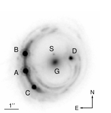
Figure 1.— HST ACS F814W image of the gravitational lens RXJ1131$-$1231. The lensed AGN images of the spiral source galaxy are marked by A, B, C and D, and the star forming regions of the spiral galaxy form the spectacular lensed structures. The primary lens galaxy and the satellite lens galaxy are indicated by G and S, respectively.

We reduce the images using MultiDrizzle with charge transfer inefficiency taken into account (e.g., Anderson & Bedin, 2010; Massey et al., 2010). The images are drizzled to a final pixel scale of $0\farcs 05$ pix^-1 and the uncertainty on the flux in each pixel is estimated from the science and the weight image by adding in quadrature the Poisson noise from the source and the background noise due to the sky and detector readout. We note that in some of the exposures the central regions of the two brightest AGN images are slightly saturated and are masked during the drizzling process.

To model the lens system using the spatially extended Einstein ring of the host galaxy, we focus on the F814W image since the contrast between the ring and the AGN is more favorable in F814W. In particular, the bright AGNs in F555W have diffraction spikes extending into the Einstein ring that are difficult to model and are thus prone to systematics effects. The detailed modeling of the F814W image is in Section 6.

4.2. Time delays

We use the new time-delay measurements of RXJ1131$-$1231 presented in Tewes et al. (2012b). The COSMOGRAIL and Kochanek et al. teams have monitored RXJ1131$-$1231 since December 2003 using several optical 1–1.5m telescopes. Resolved light curves of the four AGN images are extracted from these observations by “deconvolution photometry”, following Magain et al. (1998). These curves presently span 9 years with over 700 epochs, and display a typical sampling of 2–3 days within the observation seasons. The time delays are measured through several new and independent techniques (detailed in Tewes et al., 2012a), all specifically developed to handle microlensing variability due to stars in the lens galaxy. All these techniques yield consistent results, attributed to both the long light curves and the comprehensive uncertainty estimation. For our analysis we select the time-delay measurements from the regression difference technique as recommended by Tewes et al. (2012b) who showed that this technique yielded the smallest bias and variance in their error analysis when applied to synthetic curves mimicking the microlensing variability in RXJ1131$-$1231. In particular we use the time delays relative to image B, namely: $\Delta t_{\rm AB}=0.7\pm 1.4$ days, $\Delta t_{\rm CB}=-0.4\pm 2.0$ days, and $\Delta t_{\rm DB}=91.4\pm 1.5$ days, where the uncertainties are conservative and direct sums of the estimated statistical and systematic contributions from Tewes et al. (2012b).

4.3. Lens velocity dispersion

We observed RXJ1131$-$1231 with the Low-Resolution Imaging Spectrometer (LRIS; Oke et al. 1995) on Keck 1 on 4–5 January 2011. The data were obtained from the red side of the spectrograph using the 600/7500 grating with the D500 dichroic in place. A slit mask was employed to obtain simultaneously spectra for galaxies near the lens system. The night was clear with a nominal seeing of $0\farcs 7$, and we use 4 exposures of 1200s for a total exposure time of 4800s.

We follow Auger et al. (2008) to reduce each exposure by performing a single resampling of the spectra onto a constant wavelength grid. We use the same wavelength grid for all exposures to avoid resampling the spectra when combining them. An output pixel scale of 0.8 Å pix^-1 was used to match the dispersion of the 600/7500 grating. Individual spectra are extracted from an aperture 0$\farcs$81 wide (corresponding to 4 pixels on the LRIS red side) centered on the lens galaxy. The size of the aperture was chosen to avoid contamination from the spectrum of the lensed AGNs. We combine the extracted spectra by clipping the extreme points at each wavelength and taking the variance-weighted sum of the remaining data points. We repeat the same extraction and coaddition scheme for a sky aperture to determine the resolution of the output co-added spectrum: ${\rm R}=2300$, corresponding to $\sigma_{\rm obs}=56\,{\rm km\,s^{-1}}$. The typical signal-to-noise ratio per pixel of the final spectrum is $\sim$$20$.

The stellar velocity dispersion is determined in the same manner as Suyu et al. (2010). Briefly, we use a suite of stellar templates of K and G giants, augmented with one A and one F star template, from the INDO-US library (Valdes et al., 2004) to fit directly to the observed spectrum, after convolving each template with a kernel to bring them to the same spectral resolution as the data. First and second velocity moments are proposed by a Markov chain Monte Carlo (MCMC) simulation and the templates are shifted and broadened to these moments. We then fit the model templates to the data in a linear least squares sense, including a fifth order polynomial to account for any emission from the background source (e.g., Suyu et al., 2010). The observed and modeled spectra are shown in Figure 2. Our estimate for the central line-of-sight velocity dispersion from this inference is $\sigma=323\pm 20\,{\rm km\,s^{-1}}$, including systematics from changing the polynomial order and choosing different fitting regions.

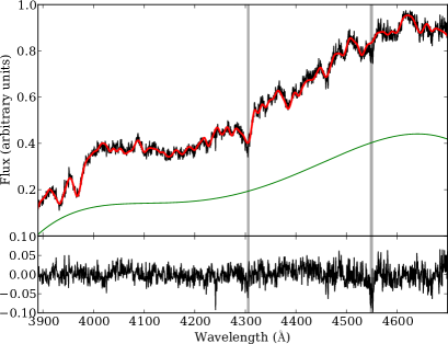
Figure 2.— Top panel: The LRIS spectrum of RXJ1131$-$1231 (black line) with a model generated from 9 INDO-US templates and a 5^th order continuum overplotted (red line, with green showing the continuum). The gray shaded areas were not included in the fit. Bottom panel: the residuals of the model fit. From the spectrum and model, we measure a central velocity dispersion of $\sigma=323\pm 20\,{\rm km\,s^{-1}}$, including systematic uncertainties.

4.4. Galaxy counts in the field

Fassnacht et al. (2011) counted the number of galaxies with F814W magnitudes between 18.5 and 24.5 that lie within $45^{\prime\prime}$ from the lens system. Compared to the aperture counts in random lines of sight in pure-parallel fields, RXJ1131$-$1231 has 1.4 times the average number of galaxy counts (Fassnacht et al., 2011). We use this relative galaxy count in Section 7.2 to estimate statistically the external convergence.

5. Probability theory for combining multiple data sets

We now present the mathematical framework for the inference of cosmological parameters from the combination of the data sets described in the previous section. In order to test for the presence of any unknown systematic uncertainty, we describe a procedure for blinding the results during the analysis phase in Section 5.2. This procedure is designed to ensure against unconscious experimenter bias towards “acceptable” results.

5.1. Joint analysis

The analysis performed here is similar to the one presented in Suyu et al. (2010), with a few improvements. We briefly describe the procedure below.

The data sets are denoted by ${d_{\rm ACS}}$ for the ACS image (packaged into a vector of $160^{2}$ surface brightness values), ${\Delta t}$ for the delays between the images, $\sigma$ for the lens velocity dispersion, and ${d_{\rm env}}$ for properties of the lens environment such as the relative galaxy count $n_{\rm r}=n_{\rm gal}/\langle n_{\rm gal}\rangle$. We are interested in obtaining the posterior PDF of the model parameters ${{\xi}}$ given all available data,

$$P(\mbox{\boldmath{${{\xi}}$}}|\mbox{\boldmath{${d_{\rm ACS}}$}},\mbox{\boldmath{${\Delta t}$}},\sigma,\mbox{\boldmath{${d_{\rm env}}$}})\propto P(\mbox{\boldmath{${d_{\rm ACS}}$}},\mbox{\boldmath{${\Delta t}$}},\sigma,\mbox{\boldmath{${d_{\rm env}}$}}|\mbox{\boldmath{${{\xi}}$}})P(\mbox{\boldmath{${{\xi}}$}})$$ (8)

where the proportionality follows from Bayes’ Theorem. The first term on the right-hand side is known as the likelihood, and the second is the prior PDF. Since the data sets are independent, the likelihood is separable,

$$P(\mbox{\boldmath{${d_{\rm ACS}}$}},\mbox{\boldmath{${\Delta t}$}},\sigma,\mbox{\boldmath{${d_{\rm env}}$}}|\mbox{\boldmath{${{\xi}}$}}) = P(\mbox{\boldmath{${d_{\rm ACS}}$}}|\mbox{\boldmath{${{\xi}}$}})\,P(\mbox{\boldmath{${\Delta t}$}}|\mbox{\boldmath{${{\xi}}$}})$$ (9)

$$\ \ \ \ P(\sigma|\mbox{\boldmath{${{\xi}}$}})\,P(\mbox{\boldmath{${d_{\rm env}}$}}|\mbox{\boldmath{${{\xi}}$}}).$$

Some of the parameters influence all the predicted data sets, while other parameters affect the fitting of particular data sets only. Specifically, $\mbox{\boldmath{${{\xi}}$}}=\{\mbox{\boldmath{${{\pi}}$}},\gamma^{\prime},\theta_{\rm E},\gamma_{\rm ext},\mbox{\boldmath{${{\eta}}$}},r_{\rm ani},\kappa_{\rm ext}\}$, where ${{\pi}}$ are the cosmological parameters (e.g., $H_{0}$, $w$, $\Omega_{\rm de}$), $\gamma^{\prime}$ is the radial profile slope of the main lens galaxy (where $\rho\propto r^{-\gamma^{\prime}}$), $\theta_{\rm E}$ is the Einstein radius of the main lens (that characterizes the normalization of the lens mass profile), $\gamma_{\rm ext}$ is the external shear strength at the lens, ${{\eta}}$ denotes the remaining lens model parameters for the ACS data, $r_{\rm ani}$ is the anisotropy radius for the stellar orbits of the lens galaxy, and $\kappa_{\rm ext}$ is the external convergence. For the lensing and time delays, we subsume the cosmological dependence into the time-delay distance $D_{\Delta t}=D_{\Delta t}(\mbox{\boldmath{${{\pi}}$}})$. Keeping only the direct dependencies in each of the likelihoods, we obtain

$$P(\mbox{\boldmath{${{\xi}}$}}|\mbox{\boldmath{${d_{\rm ACS}}$}},\mbox{\boldmath{${\Delta t}$}},\sigma,\mbox{\boldmath{${d_{\rm env}}$}})\propto P(\mbox{\boldmath{${d_{\rm ACS}}$}},\mbox{\boldmath{${\Delta t}$}}|D_{\Delta t},\gamma^{\prime},\theta_{\rm E},\gamma_{\rm ext},$$

$$\mbox{\boldmath{${{\eta}}$}},\kappa_{\rm ext})P(\sigma|\mbox{\boldmath{${{\pi}}$}},\gamma^{\prime},\theta_{\rm E},r_{\rm ani},\kappa_{\rm ext})P(\mbox{\boldmath{${d_{\rm env}}$}}|\kappa_{\rm ext},\gamma_{\rm ext})$$

$$P(\mbox{\boldmath{${{\pi}}$}})P(\gamma^{\prime})P(\theta_{\rm E})P(\gamma_{\rm ext})P(\mbox{\boldmath{${{\eta}}$}})P(r_{\rm ani})P(\kappa_{\rm ext}).$$ (10)

For cosmography, we are interested in the cosmological parameters ${{\pi}}$ after marginalizing over all other parameters

$$P(\mbox{\boldmath{${{\pi}}$}}|\mbox{\boldmath{${d_{\rm ACS}}$}},\mbox{\boldmath{${\Delta t}$}},\sigma,\mbox{\boldmath{${d_{\rm env}}$}})=\int{\rm d}\gamma^{\prime}\,{\rm d}\theta_{\rm E}\,{\rm d}\gamma_{\rm ext}\,{\rm d}\mbox{\boldmath{${{\eta}}$}}\,{\rm d}r_{\rm ani}\,$$

$${\rm d}\kappa_{\rm ext}\,P(\mbox{\boldmath{${{\xi}}$}}|\mbox{\boldmath{${d_{\rm ACS}}$}},\mbox{\boldmath{${\Delta t}$}},\sigma,\mbox{\boldmath{${d_{\rm env}}$}})$$ (11)

We describe the forms of the partially marginalized lensing and time-delay likelihood in Section 6, the kinematics likelihood in Section 7.1 and the external convergence likelihood in Section 7.2. For marginalizing the parameters that are common to the data sets, we importance sample the priors following Lewis & Bridle (2002) and Suyu et al. (2010) (a procedure sometimes referred to as “simple Monte Carlo”).

5.2. Blind analysis

We blind the analysis to avoid experimenter bias, allowing us to test for the presence of residual systematics in our analysis technique by comparing the final unblinded results from RXJ1131$-$1231 with the constraints from the previous analysis of B1608$+$656. As described by Conley et al. (2006), the blinding is not meant to hide all information from the experimenter; rather, we blind only the parameters that concern the cosmological inference.

We define two analysis phases. During the initial “blind” phase, we compute likelihoods and priors, and sample the posterior PDF, as given above, taking care to only make parameter-space plots using one plotting code. This piece of software adds offsets to the cosmological parameters ($D_{\Delta t}$ and the components of ${{\pi}}$) before displaying the PDFs, such that we always see the marginalized distributions with centroids at exactly zero. We can therefore still see, and measure, the precision of the blinded parameters, and visualize the correlations between these parameters, but without being able to see if we have “the right answer” based on our expectations. Both the parameter uncertainties and degeneracies serve as useful checks during this blind phase: the plotting routine can overlay the constraints from different models to investigate sources of statistical and systematic uncertainties.

During the blind phase we performed a number of tests on the modeling to quantify the sources of uncertainties, and to check the robustness of the results. These are described in Sections 4–8. At the end of the tests, the collaboration convened a telecon to unblind the results. The authors SHS, MWA, SH, PJM, MT, TT, CDF, LVEK, DS, and FC discussed in detail the analysis and the blinded results, over a summary website. After all agreeing that the blind analysis was complete, and that we would publish without modification the results once unblinded, a script was run to update automatically the same website with plots and tables containing cosmological constraints no longer offset to zero. These are the results presented in Sections 8 and 9.1.

6. Lens Modeling

In this section, we simultaneously model the ACS images and the time delays to measure the lens model parameters, particularly $D_{\Delta t}$, $\gamma^{\prime}$, $\theta_{\rm E}$, and $\gamma_{\rm ext}$.

6.1. A comprehensive mass and light model

The ACS image in Figure 1 shows the light from the source as lensed by the galaxies G and S. To predict the surface brightness of the pixels on the image, we need a model for the lens mass distribution (that deflects the light of the source), the lens light distribution, the source light distribution and the point spread function (PSF) of the telescope.

6.1.1 Lens mass profiles

We use elliptically-symmetric distributions with power-law profiles to model the dimensionless surface mass density of the lens galaxies,

$$\kappa_{\rm pl}(\theta_{1},\theta_{2})=\frac{3-\gamma^{\prime}}{2}\left(\frac{\theta_{\rm E}}{\sqrt{q\theta_{1}^{2}+\theta_{2}^{2}/q}}\right)^{\gamma^{\prime}-1},$$ (12)

where $\gamma^{\prime}$ is the radial power-law slope (with $\gamma^{\prime}=2$ corresponding to isothermal), $\theta_{\rm E}$ is the Einstein radius, and $q$ is the axis ratio of the elliptical isodensity contours. Various studies have shown that the power-law profile provides accurate descriptions of lens galaxies (e.g., Gavazzi et al., 2007; Humphrey & Buote, 2010; Koopmans et al., 2009; Auger et al., 2010; Barnabè et al., 2011). In particular, Suyu et al. (2009) found that the grid-based lens potential corrections from power-law models were only $\sim 2\%$ for B1608$+$656 with interacting lens galaxies, thus validating the use of the simple power-law models even for complicated lenses. We note that the surface brightness of the main deflector in RXJ1131$-$1231 shows no signs of interaction (Section 6.1.2) and it is therefore much simpler than the case of B1608$+$656, further justifying the use of a simple power-law model to describe the mass distribution within the multiple images.

The Einstein radius in Equation (12) corresponds to the geometric radius of the critical curve, and the mass enclosed within the isodensity contour with the geometric Einstein radius is

$$M_{\rm E}=\pi\theta_{\rm E}^{2}D_{\rm d}^{2}\Sigma_{\rm crit}$$ (13)

that depends only on $\theta_{\rm E}$, a robust quantity in lensing.

The deflection angle and lens potential of the power-law profile are computed following Barkana (1998). For each lens galaxy, the distribution is suitably translated to the position of the lens galaxy and rotated by the position angle $\phi$ of the lens galaxy (where $\phi$ is a free parameter, measured counterclockwise from $\theta_{2}$). Since the satellite galaxy is small in extent, we approximate its mass distribution as a spherical isothermal mass distribution with $\gamma^{\prime}_{\rm S}=2$ and $q_{\rm S}=1$ in Equation (12). The (very small) impact of the satellite on cosmographic inferences is discussed in Section 8.5.

Our coordinate system is defined such that $\theta_{1}$ and $\theta_{2}$ point to the west and north, respectively. The origin of the coordinates is at the bottom-left corner of the ACS image containing 160$\times$160 pixels.

In addition to the lens galaxies, we include a constant external shear of the following form in polar coordinates $\theta$ and $\varphi$:

$$\psi_{\rm ext}(\theta,\varphi)=\frac{1}{2}\gamma_{\rm ext}\theta^{2}\cos 2(\varphi-\phi_{\rm ext}),$$ (14)

where $\gamma_{\rm ext}$ is the shear strength and $\phi_{\rm ext}$ is the shear angle. The shear position angle of $\phi_{\rm ext}=0\arcdeg$ corresponds to a shearing along the $\theta_{1}$ direction whereas $\phi_{\rm ext}=90\arcdeg$ corresponds to a shearing in the $\theta_{2}$ direction.

We do not include the external convergence $\kappa_{\rm ext}$ at this stage, since this parameter is completely degenerate with $D_{\Delta t}$ in the ACS and time-delay modeling. Rather, we use $D_{\Delta t}^{\rm model}\equiv(1-\kappa_{\rm ext})D_{\Delta t}$ for the lensing and time-delay data, and information on $\kappa_{\rm ext}$ will come from kinematics and lens environment in Section 7 to allow us to infer $D_{\Delta t}$.

6.1.2 Lens light

For the light distribution of the lens galaxies, we use elliptical Sérsic profiles,

$$I(\theta_{1},\theta_{2})=A\exp\left[-k\left(\left(\frac{\sqrt{\theta_{1}^{2}+\theta_{2}^{2}/q_{\rm L}^{2}}}{R_{\rm eff}}\right)^{1/n_{\rm sersic}}-1\right)\right],$$ (15)

where $A$ is the amplitude, $k$ is a constant such that $R_{\rm eff}$ is the effective (half-light) radius, $q_{\rm L}$ is the axis ratio, and $n_{\rm sersic}$ is the Sérsic index (Sérsic, 1968). The distribution is suitably rotated by positions angle $\phi_{\rm L}$ and translated to the galaxy positions $(\theta_{1,L},\theta_{2,L})$. We find that a single Sérsic profile for the primary lens galaxy leads to significant residuals, as was found by Claeskens et al. (2006). Instead, we use two Sérsic profiles with common centroids and position angles to describe the lens galaxy G. For the small satellite galaxy that illuminates only a few pixels, we use a circular Sérsic profile with $n_{\rm sersic}=1$. This simplifying assumption has no effect on the mass modeling since the light of the satellite is central and compact, and thus does not affect the light or mass of the other components.

6.1.3 Source light

To describe the surface brightness distribution of the lensed source, we follow Suyu (2012) and use a hybrid model comprised of (1) point images for the lensed AGNs on the image plane, and (2) a regular grid of source surface brightness pixels for the spatially extended AGN host galaxy. Modeling the AGN point images independently accommodates variations in the fluxes arising from microlensing, time delays and substructures. Each AGN image therefore has three parameters: a position in $\theta_{1}$ and $\theta_{2}$ and an amplitude. We collectively denote these AGN parameters as ${\nu}$. The extended source on a grid is modeled following Suyu et al. (2006), with curvature regularization.

6.1.4 PSF

A PSF is needed to model the light of the lens galaxies and the lensed source. We use stars in the field to approximate the PSF, which has been shown to work sufficiently well in modeling galaxy-scale strong lenses (e.g., Marshall et al., 2007; Suyu et al., 2009; Suyu, 2012). In particular, we adopt the star that is located at $2\farcm 4$ northwest of the lens system as the model of the PSF.

6.1.5 Image pixel uncertainties

The comprehensive mass and light model described above captures the large-scale features of the data very well. However, small-scale features in the image might cause misfits which, if not taken into account, may lead to an underestimation of parameter uncertainties and biased parameter estimates. Suyu (2012) found that by boosting the pixel uncertainty of the image surface brightness, the lens model parameters can be faithfully recovered with realistic estimation of uncertainties.

Following this study, we introduce two terms to describe the variance of the intensity at pixel $i$ of the ACS image ${d_{\rm ACS}}$,

$$\sigma_{{\rm pix},i}^{2}=\sigma_{\rm bkgd}^{2}+fd_{{\rm ACS,}i},$$ (16)

where $\sigma_{\rm bkgd}$ is the background uncertainty, $f$ is a scaling factor, and $d_{{\rm ACS,}i}$ is the image intensity. The second term, $fd_{{\rm ACS,}i}$, corresponds to a scaled version of Poisson noise for the astrophysical sources. We measure $\sigma_{\rm bkgd}$ from a blank region in the image without astrophysical sources. We set the value of $f$ such that the reduced $\chi^{2}$ is $\sim$1 for the lensed image reconstruction (see, e.g., Suyu et al., 2006, for details on the computation of the reduced $\chi^{2}$ that takes into account the regularization on the source pixels). Equation (16) by design downweights regions of high intensities where the residuals are typically most prominent. This allows the lens model to fit to the overall structure of the data instead of reducing high residuals at a few locations at the expense of poorer fits to the large-scale lensing features. The residuals near the AGN image positions are particularly high due to the high intensities and slight saturations in some of the images. Therefore, we set the uncertainty on the inner pixels of the AGN images to a very large number that effectively leads to these pixels being discarded. We discard only a small region in fitting the AGN light, and increase the region to minimize AGN residuals when using the extended source features to constrain the lens mass parameters.

6.2. Likelihoods

The model-predicted image pixel surface brightness can be written as a vector

$$\mbox{\boldmath{${d_{\rm ACS}^{\rm P}}$}}=\mbox{\boldmath{${\mathsf{B}}$}}\mbox{\boldmath{${g}$}}+\mbox{\boldmath{${\mathsf{B}}$}}\mbox{\boldmath{${\mathsf{L}}$}}\mbox{\boldmath{${s}$}}+\sum_{i=1}^{N_{\rm AGN}}\mbox{\boldmath{${a}$}}_{i}(\mbox{\boldmath{${\nu}$}}),$$ (17)

where ${\mathsf{B}}$ is a blurring operator that accounts for the PSF convolution, ${g}$ is a vector of image pixel intensities of the Sérsic profiles for the lens galaxy light, ${\mathsf{L}}$ is the lensing operator that maps source intensity to the image plane based on the deflection angles computed from the parameters of the lens mass distributions (such as $\gamma^{\prime}$, $\theta_{\rm E}$, $\gamma_{\rm ext}$), ${s}$ is a vector of source-plane pixel intensities, $N_{\rm AGN}(=4)$ is the number of AGN images, and $\mbox{\boldmath{${a}$}}_{i}(\mbox{\boldmath{${\nu}$}})$ is the vector of image pixel intensities for PSF-convolved image $i$ of the AGN.

The likelihood of the ACS data with $N_{\rm d}$ image pixels is

$$P(\mbox{\boldmath{${d_{\rm ACS}}$}}|\gamma^{\prime},\theta_{\rm E},\gamma_{\rm ext},\mbox{\boldmath{${{\eta}}$}})$$ (18)

$$=\int{\rm d}\mbox{\boldmath{${s}$}}\,P(\mbox{\boldmath{${d_{\rm ACS}}$}}|\gamma^{\prime},\theta_{\rm E},\gamma_{\rm ext},\mbox{\boldmath{${{\eta}}$}},\mbox{\boldmath{${s}$}})P(\mbox{\boldmath{${s}$}}),$$

where

$$P(\mbox{\boldmath{${d_{\rm ACS}}$}}|\gamma^{\prime},\theta_{\rm E},\gamma_{\rm ext},\mbox{\boldmath{${{\eta}}$}},\mbox{\boldmath{${s}$}})=$$ (19)

$$\frac{1}{Z_{\rm d}}\exp\sum_{i=1}^{N_{\rm d}}\left[-\frac{\left(d_{{\rm ACS,}i}-d_{{\rm ACS,}i}^{\rm P}\right)^{2}}{2\sigma_{{\rm pix},i}^{2}}\right]$$

$$\cdot\prod_{i}^{N_{\rm AGN}}\frac{1}{\sqrt{2\pi}\sigma_{i}}\exp\left[-\frac{|\mbox{\boldmath{${\theta}$}}_{i}-\mbox{\boldmath{${\theta}$}}^{\rm P}_{i}|^{2}}{2\sigma_{i}^{2}}\right].$$

In the first term of this likelihood function, $Z_{\rm d}$ is just the normalization

$$Z_{\rm d}=(2\pi)^{N_{\rm d}/2}\prod_{i=1}^{N_{\rm d}}\sigma_{{\rm pix},i},$$ (20)

$d_{{\rm ACS,}i}$ is the surface brightness of pixel $i$, $d_{{\rm ACS,}i}^{\rm P}(\gamma^{\prime},\theta_{\rm E},\gamma_{\rm ext},\mbox{\boldmath{${{\eta}}$}},\mbox{\boldmath{${s}$}})$ is the corresponding predicted value given by Equation (17) (recall that ${{\eta}}$ are the remaining lens model parameters to which the ACS data are sensitive), and $\sigma_{{\rm pix},i}^{2}$ is the pixel uncertainty given by Equation (16). The second term in the likelihood accounts for the positions of the AGN images, modeled as independent points (i.e. non-pixelated sources) in the image. In this term, $\mbox{\boldmath{${\theta}$}}_{i}$ is the measured image position (listed in Table 1), $\sigma_{i}$ is the estimated positional uncertainty of $0.005^{\prime\prime}$, and $\mbox{\boldmath{${\theta}$}}^{\rm P}_{i}(\gamma^{\prime},\theta_{\rm E},\gamma_{\rm ext},\mbox{\boldmath{${\eta}$}})$ is the predicted image position given the lens parameters. (Notice that this second term does not contribute to the marginalization integral of Equation (18).) The form of $P(\mbox{\boldmath{${s}$}})$ for the source intensity pixels and the resulting analytic expression for the marginalization in Equation (18) are detailed in Suyu et al. (2006).

Table 1Lens model parameters

		Marginalized
Description	Parameter	or optimized
		constraints
Time-delay distance (Mpc)	$D_{\Delta t}^{\rm model}$	$1883^{+89}_{-85}$
Lens mass distribution
Centroid of G in $\theta_{1}$ (arcsec)	$\theta_{\rm 1,G}$	$4.420^{+0.003}_{-0.002}$
Centroid of G in $\theta_{2}$ (arcsec)	$\theta_{\rm 2,G}$	$3.932^{+0.004}_{-0.003}$
Axis ratio of G	$q_{\rm G}$	$0.763^{+0.005}_{-0.008}$
Position angle of G ($\arcdeg$)	$\phi_{\rm G}$	$115.8^{+0.5}_{-0.5}$
Einstein radius of G (arcsec)	$\theta_{\rm E}$	$1.64^{+0.01}_{-0.02}$
Radial slope of G	$\gamma^{\prime}$	$1.95^{+0.05}_{-0.04}$
Centroid of S in $\theta_{1}$ (arcsec)	$\theta_{\rm 1,S}$	$4.323$
Centroid of S in $\theta_{2}$ (arcsec)	$\theta_{\rm 2,S}$	$4.546$
Einstein radius of S (arcsec)	$\theta_{\rm E,S}$	$0.20^{+0.01}_{-0.01}$
External shear strength	$\gamma_{\rm ext}$	$0.089^{+0.006}_{-0.006}$
External shear angle ($\arcdeg$)	$\phi_{\rm ext}$	$92^{+1}_{-2}$
Lens light as Sérsic profiles
Centroid of G in $\theta_{1}$ (arcsec)	$\theta_{\rm 1,GL}$	$4.411^{+0.001}_{-0.001}$
Centroid of G in $\theta_{2}$ (arcsec)	$\theta_{\rm 2,GL}$	$4.011^{+0.001}_{+0.001}$
Position angle of G ($\arcdeg$)	$\phi_{\rm GL}$	$121.6^{+0.5}_{-0.5}$
Axis ratio of G1	$q_{\rm GL1}$	$0.878^{+0.004}_{-0.003}$
Amplitude of G1	$A_{\rm GL1}$	$0.091^{+0.001}_{-0.001}$
Effective radius of G1 (arcsec)	$R_{\rm eff,GL1}$	$2.49^{+0.01}_{-0.01}$
Index of G1	$n_{\rm sersic,GL1}$	$0.93^{+0.03}_{-0.03}$
Axis ratio of G2	$q_{\rm GL2}$	$0.849^{+0.004}_{-0.004}$
Amplitude of G2	$A_{\rm GL2}$	$0.89^{+0.03}_{-0.03}$
Effective radius of G2 (arcsec)	$R_{\rm eff,GL2}$	$0.362^{+0.009}_{-0.009}$
Index of G2	$n_{\rm sersic,GL2}$	$1.59^{+0.03}_{-0.03}$
Centroid of S in $\theta_{1}$ (arcsec)	$\theta_{\rm 1,SL}$	$4.323$
Centroid of S in $\theta_{2}$ (arcsec)	$\theta_{\rm 2,SL}$	$4.546$
Axis ratio of S	$q_{\rm SL}$	$\equiv 1$
Amplitude of S	$A_{\rm SL}$	$34.11$
Effective radius of S (arcsec)	$R_{\rm eff,SL}$	$0.01$
Index of S	$n_{\rm sersic,SL}$	$\equiv 1$
Lensed AGN light
Position of image A in $\theta_{1}$ (arcsec)	$\theta_{\rm 1,A}$	$2.383$
Position of image A in $\theta_{2}$ (arcsec)	$\theta_{\rm 2,A}$	$3.412$
Amplitude of image A	$a_{\rm A}$	$1466$
Position of image B in $\theta_{1}$ (arcsec)	$\theta_{\rm 1,B}$	$2.344$
Position of image B in $\theta_{2}$ (arcsec)	$\theta_{\rm 2,B}$	$4.594$
Amplitude of image B	$a_{\rm B}$	$1220$
Position of image C in $\theta_{1}$ (arcsec)	$\theta_{\rm 1,C}$	$2.960$
Position of image C in $\theta_{2}$ (arcsec)	$\theta_{\rm 2,C}$	$2.300$
Amplitude of image C	$a_{\rm C}$	$502$
Position of image D in $\theta_{1}$ (arcsec)	$\theta_{\rm 1,D}$	$5.494$
Position of image D in $\theta_{2}$ (arcsec)	$\theta_{\rm 2,D}$	$4.288$
Amplitude of image D	$a_{\rm D}$	$129$

Notes. There are a total of 39 parameters that are optimized or sampled. Parameters that are optimized are held fixed in the sampling of the full parameter space and have no uncertainties tabulated. Changes in these optimized parameters have little effect on the key parameters for cosmology (such as $D_{\Delta t}^{\rm model}$). The tabulated values for the sampled parameters are the marginalized constraints with uncertainties given by the $16^{\rm th}$ and $84^{\rm th}$ percentiles (to indicate the 68% credible interval). For the lens light, two Sérsic profiles with common centroid and position angle are used to describe the primary lens galaxy G. They are denoted as G1 and G2 above. The position angles are measured counterclockwise from positive $\theta_{2}$ (north). The source surface brightness of the AGN host is modeled on a grid of pixels; these pixel parameters (${s}$) are analytically marginalized and are thus not listed.

The likelihood for the time delays is given by

$$P(\mbox{\boldmath{${\Delta t}$}}|D_{\Delta t}^{\rm model},\gamma^{\prime},\theta_{\rm E},\gamma_{\rm ext},\mbox{\boldmath{${{\eta}}$}})=$$ (21)

$$\prod_{i}\left(\frac{1}{\sqrt{2\pi}\sigma_{\Delta t,i}}\exp\left[\frac{(\Delta t_{i}-\Delta t_{i}^{\rm P})^{2}}{2\sigma_{\Delta t,i}^{2}}\right]\right),$$

where $\Delta t_{i}$ is the measured time delay with uncertainty $\sigma_{\Delta t,i}$ for image pair $i$=AB, CB, or DB, and $\Delta t_{i}^{\rm P}(D_{\Delta t}^{\rm model},\gamma^{\prime},\theta_{\rm E},\gamma_{\rm ext},\mbox{\boldmath{${{\eta}}$}})$ is the corresponding predicted time delay computed via Equation (6) given the lens mass model parameters.

The joint likelihood for the ACS and time delay data that appears in Equation (5.1), $P(\mbox{\boldmath{${d_{\rm ACS}}$}},\mbox{\boldmath{${\Delta t}$}}|D_{\Delta t},\gamma^{\prime},\theta_{\rm E},\gamma_{\rm ext},\mbox{\boldmath{${{\eta}}$}},\kappa_{\rm ext})$, is just the product of the likelihoods in Equations (18) and (21).

We assign uniform priors over reasonable linear ranges for all the lens parameters: $D_{\Delta t}^{\rm model}$, $\gamma^{\prime}$, $\theta_{\rm E}$, $\gamma_{\rm ext}$ and ${{\eta}}$. In particular, for the first four lens parameters, the linear ranges for the priors are $D_{\Delta t}^{\rm model}\in[0,10000]\,{\rm Mpc}$, $\gamma^{\prime}\in[1.5,2.5]$, $\theta_{\rm E}\in[0,5]^{\prime\prime}$, and $\gamma_{\rm ext}\in[0,1]$.

6.3. MCMC sampling

Figure 3.— Posterior of the key lens model parameters for the lensing and time-delay data. Each color represents a particular source resolution that is the dominant systematic uncertainty in the modeling of the ACS data. The solid curves are a Gaussian fit to the PDF by weighting each source resolution chain equally. The contours/shades mark the 68.3%, 95.4%, 99.7% credible regions.

We model the ACS image and time delays with Glee, a software package developed by Suyu & Halkola (2010) based on Suyu et al. (2006) and Halkola et al. (2008). The ACS image has $160$$\times$$160$ surface brightness pixels as constraints. There are a total of 39 lens model parameters that are summarized in Table 1. This is the most comprehensive lens model of RXJ1131$-$1231 to date. The list of parameters excludes the source surface brightness pixel parameters, ${s}$, which are analytically marginalized in computing the likelihood (see, e.g., Suyu & Halkola, 2010, for details). With such a large parameter space, we sequentially sample individual parts of the parameter space first to get good starting positions near the peak of the PDF before sampling the full parameter space. The aim is to obtain a robust PDF for the key lens parameters for cosmography: $D_{\Delta t}^{\rm model}$, $\gamma^{\prime}$, $\theta_{\rm E}$, and $\gamma_{\rm ext}$.

For an initial model of the lens light, we create an annular mask for the lensed arc and use the image pixels outside the annular mask to optimize the lens Sérsic profiles. The parameters for the light of the satellite is fixed to these optimized values for the remainder of the analysis since the satellite light has negligible effect on $D_{\Delta t}^{\rm model}$ and other lens parameters. Furthermore, we fix the centroid of the satellite’s mass distribution to its observed light centroid. We obtain an initial mass model for the lenses using the image positions of the multiple knots in the source that are identified following Brewer & Lewis (2008). Specifically, we optimize for the parameters that minimize the separation between the identified image positions and the predicted image positions from the mass model. We then optimize the AGN light together with the light of the extended source while keeping the lens light and lens mass model fixed. The AGN light parameters are then held fixed to these optimized values. Having obtained initial values for all the lens model parameters to describe the ACS data, we then proceed to sample the lens parameters listed in Table 1 using a MCMC method. In particular, we simultaneously vary the following parameters: modeled time-delay distance, all mass parameters of G, the Einstein radius of S, external shear, the extended source intensity distribution, and the lens light profile of G. Glee employs several of the methods of Dunkley et al. (2005) for efficient MCMC sampling and for assessing chain convergence.

6.4. Constraints on the lens model parameters

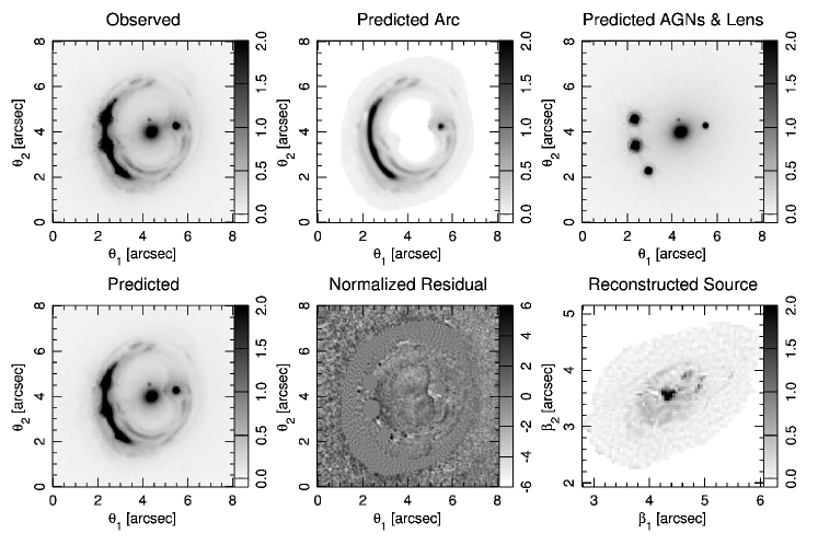
Figure 4.— ACS image reconstruction of the most probable model with a source grid of 64$\times$64 pixels. Top left: observed ACS F814W image. Top middle: predicted lensed image of the background AGN host galaxy. Top right: predicted light of the lensed AGNs and the lens galaxies. Bottom left: predicted image from all components, which is a sum of the top-middle and top-right panels. Bottom middle: image residual, normalized by the estimated 1$\sigma$ uncertainty of each pixel. Bottom right: the reconstructed host galaxy of the AGN in the source plane. Our lens model reproduces the global features of the data.

We explore various parameter values for the AGN light and the satellite Sérsic light, try different PSF models, and consider different masks for the lensed arcs and the AGNs (which are fixed in the MCMC sampling). These variations have negligible effect on the sampling of the other lens parameters. The only attribute that changes the PDF of the parameters significantly is the number of source pixels, or equivalently, the source pixel size. We try a series of source resolution from coarse to fine, and the parameter constraints stabilize starting at $\sim$50$\times$50 source pixels, corresponding to source pixel sizes of $\sim$$0\farcs 05$. Nonetheless, the parameter constraints for different source resolutions are shifted significantly from one another. Different source pixelizations minimize the image residuals in different manners, and predict different relative thickness of the arcs that provides information on the lens profile slope $\gamma^{\prime}$ (e.g., Suyu, 2012). To quantify this systematic uncertainty, we consider the following set of source resolutions: $50$$\times$$50$, $52$$\times$$52$, $54$$\times$$54$, $56$$\times$$56$, $58$$\times$$58$, $60$$\times$$60$, and $64$$\times$$64$. The likelihood $P(\mbox{\boldmath{${d_{\rm ACS}}$}},\mbox{\boldmath{${\Delta t}$}}|D_{\Delta t}^{\rm model},\gamma^{\prime},\theta_{\rm E},\gamma_{\rm ext})$, which is proportional to the marginalized posterior of these parameters $P(D_{\Delta t}^{\rm model},\gamma^{\prime},\theta_{\rm E},\gamma_{\rm ext}|\mbox{\boldmath{${d_{\rm ACS}}$}},\mbox{\boldmath{${\Delta t}$}})$ since the priors are uniform, is plotted in Figure 3 for each of these source resolutions. The scatter in constraints among the various source resolutions allows us to quantify the systematic uncertainty. In particular, we weight each choice of the source resolution equally, and combine the Markov chains together. In Table 1, we list the marginalized parameters from the combined samples.

We show the most probable image and source reconstruction for the $64$$\times$$64$ resolution in Figure 4. Only the image intensity pixels within the annular mask shown in the top-middle panel are used to reconstruct the source that is shown in the bottom-right panel. A comparison of the top-left and bottom-left panels shows that our lens model reproduces the global features of the ACS image. The time delays are also reproduced by the model: for the various source resolutions, the $\chi^{2}$ (not reduced) is $\sim$2 for the three delays relative to image B. There are some small residual features in the bottom-middle panel of Figure 4, and these cause the shifts in the parameter constraints seen in Figure 3 for different source pixel sizes. The reconstructed host galaxy of the AGN in the bottom-right panel shows a compact central peak, which is probably the bulge of the spiral source galaxy, embedded in a more diffuse patch of light (the disk) with knots/spiral features. The bulge and disk have half-light radii of $\sim$$0\farcs 1$ and $\sim$$0\farcs 8$, respectively. Given the source redshift, this implies a bulge size of $\sim$0.7 kpc and a disk size of $\sim$5 kpc, which are typical for disk galaxies at these redshifts (e.g., Barden et al., 2005; MacArthur et al., 2008) and are comparable to the largest sources in the lens systems of the Sloan Lens ACS survey (Newton et al., 2011).

6.5. Understanding the external shear

The inferred external shear is $\gamma_{\rm ext}=0.089\pm 0.006$ (marginalizing over all other model parameters) from modeling the ACS image and the time delays. The external shear may provide information on the amount of external convergence, since they originate from the same external structures. However, the high $\gamma_{\rm ext}$ found in our model could potentially be attributed to deviations of the primary lens from its elliptical power-law description; if this were the case, some of $\gamma_{\rm ext}$ would in fact be internal shear. To gauge whether the modeled shear is truly external, we also considered a model that includes a constant external convergence gradient. This introduces two additional parameters: $\kappa^{\prime}$ (gradient) and $\phi_{\kappa}$ (the position angle of the gradient, where $\phi_{\kappa}=0$ corresponds to positive $\kappa$ gradient along the positive $\theta_{2}$ direction, i.e., north). The ACS data allow us to constrain $\kappa^{\prime}=(5.1^{+0.4}_{-0.3})\times 10^{-3}\,\rm{arcsec}^{-1}$ and $\phi_{\kappa}=87\pm 2\arcdeg$. The convergence gradient is aligned along the same direction as the external shear within $5\arcdeg$ and has a sensible magnitude, suggesting that the shear is in fact truly external, and is likely due to mass structures to the east of the lens.

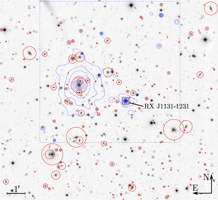
Figure 5.— $11.5^{\prime}$$\times$$10.5^{\prime}$ R-band image obtained from stacking 60 hours of the best-quality images in the COSMOGRAIL monitoring. The lens system is marked by the box near the center. Galaxies (stars) in the field are indicated by solid (dashed) circles. The radius of the solid circle is proportional to the flux of the galaxy. X-ray map from Chartas et al. (2009) are overlaid on the image within the dashed box. The concentrations of mass structures to the east of the lens are consistent with the modeled external shear and convergence gradient directions.

To investigate the origin of the external shear, we construct a wide-field R-band image from the COSMOGRAIL monitoring images that is shown in Figure 5. The lens system is indicated by the box, and the galaxies (stars) in the field are marked by solid (dashed) circles, identified using SExtractor (Bertin & Arnouts, 1996). Overlaid on the image within the dashed box are the X-ray contours from Chartas et al. (2009), showing the presence of a galaxy cluster that is located at $158^{\prime\prime}$ northeast of the lens (Morgan et al., 2006; Chartas et al., 2009). The cluster is at $z=0.1$ based on the redshift measurements of two of the red-sequence cluster galaxies from the Las Campanas Redshift Survey (Shectman et al., 1996; Williams et al., 2006). Using the measured 2$-$10 keV luminosity of $1.7\times 10^{42}{\rm\,ergs\,s^{-1}}$, X-ray temperature of 1.2 keV and core radius of a $\beta$ model of $4.2^{\prime\prime}$ for the cluster (Chartas et al., 2009), we estimate that the contribution of the cluster to the external shear at the lens is only a few percent. Nonetheless, large-scale structures associated with the cluster and the plethora of mass structures to the east of the lens could generate additional shear. The fact that our modeled external shear and convergence gradients both point toward mass structures in the east that are visible in Figure 5 is a further indication that the modeled shear is indeed external. We will use this external shear in Section 7.2 to constrain the external convergence.

6.6. Propagating the lens model forward

To facilitate the sampling and marginalization of the posterior of the cosmological parameters in Equations (5.1) and (5.1), we approximate the overall likelihood of ${d_{\rm ACS}}$ and ${\Delta t}$ from the multiple source resolutions in Figure 3 with a multivariate Gaussian distribution for the interesting parameters $\gamma^{\prime},\theta_{\rm E},\gamma_{\rm ext}$ and $D_{\Delta t}^{\rm model}$, marginalizing over the nuisance parameters ${{\eta}}$. This approximation allows the value of $P(\mbox{\boldmath{${d_{\rm ACS}}$}},\mbox{\boldmath{${\Delta t}$}}|\gamma^{\prime},\theta_{\rm E},\gamma_{\rm ext},D_{\Delta t}^{\rm model})$ to be computed at any position in this 4-dimensional parameter space. Note that in contrast to the other parameters, the Einstein radius of the primary lens galaxy, $\theta_{\rm E}$, is well determined, with minimal degeneracy with other parameters. This robust quantity is used in the dynamics modeling of the lens galaxy. The approximated Gaussian likelihood provides an easy way to combine with the stellar kinematics and lens environment information for measuring $D_{\Delta t}$.

7. Constraining the external convergence $\kappa_{\rm ext}$

In this section, we fold in additional information on the lens galaxy stellar kinematics and density environment to constrain the nuisance parameter $\kappa_{\rm ext}$ (which characterizes the effects of LOS structures).

7.1. Stellar kinematics

We follow Suyu et al. (2010) and model the velocity dispersion of the stars in the primary lens galaxy G, highlighting the main steps. The three-dimensional mass density distribution of the lens galaxy can be expressed as

$$\rho_{\rm G}(r)=(\kappa_{\rm ext}-1)\Sigma_{\rm crit}\theta_{\rm E}^{\gamma^{\prime}-1}D_{\rm d}^{\gamma^{\prime}-1}\frac{\Gamma(\frac{\gamma^{\prime}}{2})}{\pi^{1/2}\Gamma(\frac{\gamma^{\prime}-3}{2})}\frac{1}{r^{\gamma^{\prime}}}.$$ (22)

Note that the projected mass of the lens galaxy enclosed within $\theta_{\rm E}$ is $(1-\kappa_{\rm ext})M_{\rm E}$, while the projected mass associated with the external convergence is $\kappa_{\rm ext}M_{\rm E}$; the sum of the two is the Einstein mass $M_{\rm E}$ that was given in Equation (13). We employ spherical Jean’s modeling to infer the line-of-sight velocity dispersion, $\sigma^{\rm P}(\mbox{\boldmath{${{\pi}}$}},\gamma^{\prime},\theta_{\rm E},r_{\rm ani},\kappa_{\rm ext})$, from $\rho_{\rm G}$ by assuming the Hernquist profile (Hernquist, 1990) for the stellar distribution (e.g., Binney & Tremaine, 1987; Suyu et al., 2010). An anisotropy radius of $r_{\rm ani}=0$ corresponds to pure radial stellar orbits, while $r_{\rm ani}\rightarrow\infty$ corresponds to isotropic orbits with equal radial and tangential velocity dispersions. We note that $\sigma^{\rm P}$ is independent of $H_{0}$, but is dependent on the other cosmological parameters (e.g.,$w$ and $\Omega_{\rm de}$) through $\Sigma_{\rm crit}$ and the physical scale radius of the stellar distribution.

The likelihood for the velocity dispersion is

$$P(\sigma|\mbox{\boldmath{${{\pi}}$}},\gamma^{\prime},\theta_{\rm E},r_{\rm ani},\kappa_{\rm ext})$$ (23)

$$=\frac{1}{\sqrt{2\pi\sigma_{\sigma}^{2}}}\exp{\left[-\frac{(\sigma-\sigma^{\rm P}(\mbox{\boldmath{${{\pi}}$}},\gamma^{\prime},\theta_{\rm E},r_{\rm ani},\kappa_{\rm ext}))^{2}}{2\sigma_{\sigma}^{2}}\right]},$$

where $\sigma=323\,\rm km\,s^{-1}$ and $\sigma_{\sigma}=20\,\rm km\,s^{-1}$ from Section 4.3. Recall that the priors on $\gamma^{\prime}$ and $\theta_{\rm E}$ were assigned to be uniform in the lens modeling. We also impose a uniform prior on $r_{\rm ani}$ in the range of $[0.5,5]R_{\rm eff}$ for the kinematics modeling, where the effective radius based on the two-component Sérsic profiles in Table 1 is $1\farcs 85$ from the photometry. The uncertainty in $R_{\rm eff}$ has negligible impact on the predicted velocity dispersion. The prior PDF for ${{\pi}}$ is discussed in Section 8.1, while the PDF for $\kappa_{\rm ext}$ is described in the next section.

7.2. Lens environment

We combine the relative galaxy counts from Section 4.4, the measured external shear in Section 6.4, and the Millennium Simulation (MS; Springel et al., 2005) to obtain an estimate of $P(\kappa_{\rm ext}|\mbox{\boldmath{${d_{\rm env}}$}},\gamma_{\rm ext},{\rm MS})$. This builds on the approach presented in Suyu et al. (2010) that used only the relative galaxy counts.

Tracing rays through the Millennium Simulation (see Hilbert et al., 2009, for details of the method), we create 64 simulated survey fields, each of solid angle $4$$\times$$4\,\mathrm{deg}^{2}$. In each field we map the convergence and shear to the source redshift $z_{\rm s}$, and catalog the galaxy content, which we derive from the galaxy model by Guo et al. (2010). For each line of sight in each simulated field, we record the convergence, shear, and relative galaxy counts in a $45^{\prime\prime}$ aperture having I-band magnitudes between 18.5 and 24.5. These provide samples for the PDF $P(\kappa_{\rm ext},\gamma_{\rm ext},\mbox{\boldmath{${d_{\rm env}}$}}|{\rm MS})$. We assume that the constructed PDF is applicable to strong-lens lines of sight, following Suyu et al. (2010) who showed that the distribution of $\kappa_{\rm ext}$ for strong lens lines of sight are very similar to that for all lines of sight.

Structures in front of the lens distort the time delays and the images of the lens/source, while structures behind the lens further affect the time delays and images of the source. However, to model simultaneously the mass distributions of the strong lens galaxies and all structures along the line of sight is well beyond current capabilities. In practice, the modeling of the strong lens galaxies is performed separately from the description of line-of-sight structures, and we approximate the effects of the lines-of-sight structures into the single correction term $\kappa_{\rm ext}$, whose statistical properties we estimate from the Millennium Simulation.

By selecting the lines of sight in the Millennium Simulation that match the properties of RXJ1131$-$1231, we can obtain $P(\mbox{\boldmath{${d_{\rm env}}$}}|\kappa_{\rm ext},\gamma_{\rm ext},{\rm MS})\,P(\kappa_{\rm ext})$ and simultaneously marginalize over $\gamma_{\rm ext}$ in Equation (5.1). We assumed a uniform prior for $\gamma_{\rm ext}$ in the lensing analysis, such that $P(\gamma_{\rm ext})$ is a constant. The lensing likelihood is the only other term that depends on $\gamma_{\rm ext}$, and from Section 6.4, the lensing likelihood provides a tight constraint on $\gamma_{\rm ext}$ that is approximately Gaussian: $0.089\pm 0.006$. We can therefore simplify part of Equation (5.1) to

∫dγ_extP($${d_{\rm ACS}} {\Delta t}$$, — D_Δt, γ’, θ_E, γ_ext, κ_ext)

$$\ \ \ \ \cdot P(\mbox{\boldmath{${d_{\rm env}}$}}|\kappa_{\rm ext},\gamma_{\rm ext},{\rm MS})$$

≃P($${d_{\rm ACS}} {\Delta t}$$, — D_Δt, γ’, θ_E, κ_ext) (24)

$$\ \ \ \ \cdot P(\mbox{\boldmath{${d_{\rm env}}$}}|\kappa_{\rm ext},\gamma_{\rm ext}=0.089\pm 0.006,{\rm MS}),$$

where the above approximation, i.e., neglecting the covariance between $\gamma_{\rm ext}$ and the other parameters in the lensing likelihood and then marginalizing $\gamma_{\rm ext}$ separately, is conservative since we would gain in precision by including the covariances with other parameters. Furthermore, by Bayes’ rule,

P($${d_{\rm env}}$$— κ_ext, γ_ext=0.089±0.006, MS) P(κ_ext)

$$\propto P(\kappa_{\rm ext}|\mbox{\boldmath{${d_{\rm env}}$}},\gamma_{\rm ext}=0.089\pm 0.006,{\rm MS}),$$ (25)

which is precisely the PDF of $\kappa_{\rm ext}$ by selecting the samples in $P(\kappa_{\rm ext},\gamma_{\rm ext},\mbox{\boldmath{${d_{\rm env}}$}}|{\rm MS})$ that satisfies ${d_{\rm env}}$ with a relative galaxy count within $1.4\pm 0.05$, and subsequently weighting these samples by the Gaussian likelihood for $\gamma_{\rm ext}$. This effective prior PDF for $\kappa_{\rm ext}$ that is constructed from the weighted samples, $P(\kappa_{\rm ext}|\mbox{\boldmath{${d_{\rm env}}$}},\gamma_{\rm ext}=0.089\pm 0.006,{\rm MS})$, is shown by the solid line in Figure 6.

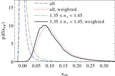
Figure 6.— The effective prior probability distribution for the external convergence $\kappa_{\rm ext}$ from combining ray tracing through the Millennium Simulation with (1) the galaxy count around the lens system relative to the average number of galaxy counts, and/or (2) the modeled external shear of $0.089\pm 0.006$. Dashed line: the convergence distribution for all lines of sight; Dot-dashed line: the convergence distribution for lines of sight with relative galaxy count $n_{\rm r}=1.4\pm 0.05$; Dotted line: the convergence distribution for all lines of sight weighted by the likelihood for $\gamma_{\rm ext}$ from the lens model; Solid line: the $\gamma_{\rm ext}$-weighted convergence distribution for lines of sight with $n_{\rm r}=1.4\pm 0.05$. The effective prior for $\kappa_{\rm ext}$ used in the final cosmological parameter inference is described by this, most informative, distribution.

8. Time-delay distance of RXJ1131$-$1231

We combine all the PDFs obtained in the previous sections to infer the time-delay distance $D_{\Delta t}$.

8.1. Cosmological priors

As written above, we could infer the time delay distance $D_{\Delta t}$ directly, given a uniform prior. However, we are primarily interested in the cosmological information contained in such a distance measurement, so prefer to infer these directly. The posterior probability distribution on $D_{\Delta t}$ can then be obtained by first calculating the posterior PDF of the cosmological parameters ${{\pi}}$ through the marginalizations in Equations (5.1) and (5.1), and then changing variables to $D_{\Delta t}$. Such transformations are of course straightforward when working with sampled PDFs.

As described in Table 2, we consider the following five cosmological world models, each with its own prior PDF $P(\mbox{\boldmath{${{\pi}}$}})$: U$H_{0}$, U$w$CDM, WMAP7$w$CDM, WMAP7o$\Lambda$CDM, and WMAP7o$w$CDM.

8.2. Posterior sampling

We sample the posterior PDF by weighting samples drawn from the prior PDF with the joint likelihood function evaluated at those points (Suyu et al., 2010). We generate samples of the cosmological parameters ${{\pi}}$ from the priors listed in Table 2. We then join these to samples of $\kappa_{\rm ext}$ drawn from $P(\kappa_{\rm ext})$ from Section 7.2 and shown in Figure 6, and to uniformly distributed samples of $\gamma^{\prime}$ within $[1.5,2.5]$ and $r_{\rm ani}$ within $[0.5,5]\,R_{\rm eff}$. Rather than generating samples of $\theta_{\rm E}$ from the uniform prior, we obtain samples of $\theta_{\rm E}$ directly from the Gaussian approximation to the lensing and time-delay likelihood since $\theta_{\rm E}$ is quite independent of other model parameters (as shown in Figure 3). This boosts sampling efficiency, and the $\theta_{\rm E}$ samples are only used to evaluate the kinematics likelihood.

For each sample of {${{\pi}}$, $\kappa_{\rm ext}$, $\gamma^{\prime}$, $r_{\rm ani}$, $\theta_{\rm E}$}, we obtain the weight (or importance) as follows: (1) we determine $D_{\Delta t}$ from ${{\pi}}$ via Equation (2), (2) we calculate $D_{\Delta t}^{\rm model}$ via Equation (7), (3) we evaluate $P(\mbox{\boldmath{${d_{\rm ACS}}$}},\mbox{\boldmath{${\Delta t}$}}|D_{\Delta t}^{\rm model},\gamma^{\prime})$ based on the Gaussian approximation shown in Figure 3 for $D_{\Delta t}^{\rm model}$ and $\gamma^{\prime}$, (4) we compute $P(\sigma|\mbox{\boldmath{${{\pi}}$}},\gamma^{\prime},\kappa_{\rm ext},\theta_{\rm E}$, $r_{\rm ani})$ via Equation (23), and (5) we weight the sample by the product of $P(\mbox{\boldmath{${d_{\rm ACS}}$}},\mbox{\boldmath{${\Delta t}$}}|D_{\Delta t}^{\rm model},\gamma^{\prime})$ and $P(\sigma|\mbox{\boldmath{${{\pi}}$}},\gamma^{\prime},\kappa_{\rm ext},\theta_{\rm E}$, $r_{\rm ani})$ from the previous two steps. The projection of these weighted samples onto ${{\pi}}$ or $D_{\Delta t}$ effectively marginalizes over the other parameters.

Table 2Priors on cosmological parameters

Prior	Description
U$H_{0}$	Flat $\Lambda$CDM with:
	uniform $H_{0}$ in $[0,150]\,\rm km\,s^{-1}\,Mpc^{-1}$,
	$\Omega_{\rm m}=0.27$, $\Omega_{\Lambda}=0.73$, $w=-1$.
	This is similar to the typical priors that
	were assumed in most of the early lensing
	studies, which sought to constrain $H_{0}$ at
	fixed cosmology.
U$w$CDM	Flat $w$CDM with:
	uniform $H_{0}$ in $[0,150]\,\rm km\,s^{-1}\,Mpc^{-1}$,
	uniform $\Omega_{\rm de}=1-\Omega_{\rm m}$ in $[0,1]$,
	uniform $w$ in $[-2.5,0.5]$.
WMAP7$w$CDM†	WMAP7 for {$H_{0}$, $\Omega_{\rm de}$, $w$} in $w$CDM
	with flatness and time-independent $w$.
WMAP7o$\Lambda$CDM†	WMAP7 for {$H_{0}$, $\Omega_{\Lambda}$, $\Omega_{\rm m}$} in open
	(or rather, non-flat) $\Lambda$CDM with $w=-1$
	and $\Omega_{\rm k}=1-\Omega_{\Lambda}-\Omega_{\rm m}$ as the curvature
	parameter.
WMAP7o$w$CDM†	WMAP7 for {$H_{0}$, $\Omega_{\rm de}$, $w$, $\Omega_{\rm k}$} in open
	$w$CDM with time-independent $w$ and
	curvature parameter $\Omega_{\rm k}=1-\Omega_{\rm de}-\Omega_{\rm m}$.

^†The prior PDF for the cosmological parameters are taken to be the posterior PDF from the WMAP 7-year data set (Komatsu et al., 2011).

8.3. Blind analysis in action

As a brief illustration of our blind analysis approach, we show in the left panel of Figure 7 the blinded plot of the time-delay distance measurement. For all cosmological parameters such as $D_{\Delta t}$, $D_{\Delta t}^{\rm model}$, $H_{0}$, $w$, $\Omega_{\rm m}$, etc., we always plotted their probability distribution with respect to the median during the blind analysis. Therefore, we could use the shape of the PDFs to check our analysis and avoid introducing experimenter bias by blinding the absolute parameter values. When we marginalized the parameters during the blind phase, our analysis code also returned the constraints with respect to the median. For example, the blinded time-delay distance for the WMAP7$w$CDM cosmology would be $0^{+130}_{-120}$ Mpc. We used this particular cosmology as our fiducial world model during the blind analysis. In the remainder of the paper, we show the unblinded results of RXJ1131$-$1231. The comparison with the gravitational lens B1608$+$656 and other cosmological probes was performed after we unblinded the analysis of RXJ1131$-$1231; otherwise, the blind analysis would be spoiled by such a comparison since the results of these previous studies were already known.

8.4. Posterior PDF for $D_{\Delta t}$

We show in the right-hand panel of Figure 7 the unblinded probability distribution of the time-delay distance for the first three cosmological models in Table 2. The priors, shown in dotted lines, are broad and rather uninformative. When including information from ${d_{\rm ACS}}$, ${\Delta t}$, $\sigma$, and $\kappa_{\rm ext}$, we obtain posterior PDFs of $D_{\Delta t}$ for RXJ1131$-$1231 that are nearly independent of the prior, demonstrating that time-delay lenses provide robust measurements of $D_{\Delta t}$. We find that the data constrain the $D_{\Delta t}$ to RXJ1131$-$1231 with $\sim$$6\%$ precision.

We can compress these results by approximating the posterior PDF for $D_{\Delta t}$ as a shifted log normal distribution:

$$P(D_{\Delta t}|H_{0},\Omega_{\rm de},w,\Omega_{\rm m})\simeq$$ (26)

$$\frac{1}{\sqrt{2\pi}(x-\lambda_{\rm D})\sigma_{\rm D}}\exp{\left[-\frac{(\log(x-\lambda_{\rm D})-\mu_{\rm D})^{2}}{2\sigma_{\rm D}^{2}}\right]},$$

where $x=D_{\Delta t}/(1\,{\rm Mpc})$, $\lambda_{\rm D}=1425.6$, $\mu_{\rm D}=6.4993$ and $\sigma_{\rm D}=0.19377$. This approximation accurately reproduces the cosmological inference, in that $H_{0}$ is recovered within $<1\%$ in terms of its median, 16^th and 84^th percentile values for the WMAP7 cosmologies we have considered. The robust constraint on $D_{\Delta t}$ serves as the basis for cosmological inferences in Section 9.

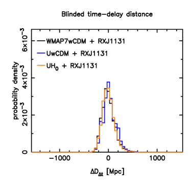
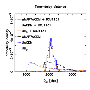
Figure 7.— Blinded (left) and unblinded (right) PDFs for $D_{\Delta t}$, showing the RXJ1131$-$1231 posterior constraints on $D_{\Delta t}$ (solid) given assorted priors for the cosmological parameters (dotted, labeled). See Table 2 for a full description of the various priors. RXJ1131$-$1231 provides tight constraints on $D_{\Delta t}$, which translates into information about $\Omega_{\rm m}$, $\Omega_{\rm de}$, $w$ and particularly $H_{0}$.

8.5. Sources of uncertainty

Our $D_{\Delta t}$ measurement accounts for all known sources of uncertainty that we have summarized in Table 3. The dominant sources are the first three items. The precision for the time delay is the 1$\sigma$ uncertainty as a fraction of the measured value for the longest delay, $\Delta t_{\rm DB}$. For the lens mass model and line-of-sight contributions, we define the precision as half the difference between the 16^th and 84^th percentiles of the PDF for $D_{\Delta t}^{\rm model}$ from Section 6.4 in fractions of its median value and for $\kappa_{\rm ext}$ from Section 7.2 in fractions of 1, respectively. The remaining sources of uncertainty are collectively denoted by “other sources”, and the two main contributors to this category are the peculiar velocity of the lens and the impact of the satellite.

Spectroscopic studies of the field of RXJ1131$-$1231 indicate that the lens is in a galaxy group with a velocity dispersion of $429^{+119}_{-93}\,\rm km\,s^{-1}$ (Wong et al., 2011). RXJ1131$-$1231 is the brightest red sequence galaxy in this group, and is thus likely to be near the center of mass of the group halo with a small peculiar velocity relative to the group (Zabludoff & Mulchaey, 1998; Williams et al., 2006; George et al., 2012). However, the group could be moving relative to the Hubble flow due to nearby large-scale structures. The one-dimensional rms galaxy peculiar velocity is typically $\lesssim 300\rm km\,s^{-1}$ (e.g., Mosquera & Kochanek, 2011; Peebles, 1993). A peculiar velocity of $300\,\rm km\,s^{-1}$ for RXJ1131$-$1231 would cause $D_{\Delta t}$ to change by $0.8\%$. A similar peculiar velocity for the lensed source has a much smaller impact on $D_{\Delta t}$, changing it by only $0.2\%$. We note that the peculiar velocities of lenses are stochastic, and this source of uncertainty should average out in a sample of lenses.

We have explicitly included the satellite in our lens mass model in Section 6. However, there is some degeneracy in apportioning the mass between the satellite and the primary lens galaxy since lensing is mostly sensitive to the total mass enclosed within the lensing critical curves (approximately traced by the arcs). The more massive the satellite, the less massive the primary lens galaxy. Owing to its central location and the degeneracy with the mass of the main deflector, we expect the impact of the satellite on the difference in gravitational potential between the multiple images to be very small.

To assess the effect of the mass of the satellite on our $D_{\Delta t}$ inference, we consider an extreme model where the satellite has zero mass. In this case, we require a more massive primary lens galaxy with higher $\theta_{\rm E}$ to fit the lensing features, as expected. The resulting $D_{\Delta t}^{\rm model}$ and $\gamma^{\prime}$ from this model are consistent with that of the original model, but with larger parameter uncertainties due to poorer fits without the satellite. Even if we use the overestimated $\theta_{\rm E}$ of the primary lens from this extreme model for the kinematics, we find that the effect on the inferred $D_{\Delta t}$ is at the $<1\%$ level.

In Table 3, we list the total uncertainty of $6.7\%$ based on a simple Gaussian approximation where we add up the uncertainties of each contribution in quadrature. This is close to the more accurate $6.0\%$ based on proper sampling that takes into account the non-Gaussian distribution (e.g., of $\kappa_{\rm ext}$) and the inclusion of the stellar velocity dispersion. We note that the sampling does not include explicitly the other sources that contribute at the $<$$1\%$ level; however, they are practically insignificant in the overall error budget. Most of the uncertainty in $D_{\Delta t}$ comes from the lens mass model and the line-of-sight contribution. Reducing the uncertainty on RXJ1131$-$1231’s $D_{\Delta t}$ would require a better model of the source intensity distribution that depends less sensitively on the source pixel size (possibly via an adaptive source pixelization scheme (e.g., Vegetti & Koopmans, 2009)), and a better characterization of $\kappa_{\rm ext}$ by using more observational information from the field. Investigations are in progress to improve $\kappa_{\rm ext}$ constraints (Greene et al., submitted; Collett et al., submitted).

Table 3Error budget on time-delay distance of RXJ1131$-$1231

Description	uncertainty
time delays	1.6%
lens mass model	4.6%
line-of-sight contribution	4.6%
other sources	$<$1%
Total (Gaussian approximation)	6.7%
Total (full sampling)	6.0%

Notes. The other sources of uncertainty that contribute at the $<$$1\%$ include the peculiar velocity of the lens and the impact of the satellite. Details are in Section 8.5. The Gaussian approximation simply adds the uncertainties in quadrature, providing a crude estimate for the total uncertainty based on the full sampling of the non-Gaussian PDFs.

9. Cosmological inference

We now present our inference on the parameters of the expanding Universe and compare our results to other cosmographic probes. Specifically, our $D_{\Delta t}$ measurement for RXJ1131$-$1231 provides information on cosmology that is illustrated in Section 9.1. We compare the results to that of B1608$+$656 to check for consistency in Section 9.2, before combining the two lenses together in Section 9.3. We then compare the constraints from the two time-delay lenses to a few other cosmological probes in Section 9.4.

9.1. Constraints from RXJ1131$-$1231

We have seen that the RXJ1131$-$1231 $D_{\Delta t}$ measurement is nearly independent of assumptions about the background cosmology. While $D_{\Delta t}$ is primarily sensitive to $H_{0}$, information from $D_{\Delta t}$ must be shared with other cosmological parameters via the combination of angular diameter distances. Therefore, cosmological parameter constraints will depend somewhat on our assumptions for the background cosmology. In this section we consider the first three cosmologies listed in Table 2: U$H_{0}$, U$w$CDM, and WMAP7$w$CDM.

With all other parameters fixed in the U$H_{0}$ cosmology except for $H_{0}$, all our knowledge of $D_{\Delta t}$ is converted to information on $H_{0}$. We therefore obtain a precise measurement of $H_{0}=78.7^{+4.3}_{-4.5}\,\rm km\,s^{-1}\,Mpc^{-1}$ for RXJ1131$-$1231 with a 5.5% uncertainty.

Next, we relax our assumptions on $\Omega_{\rm de}$, $\Omega_{\rm m}$ and $w$, and consider the U$w$CDM and WMAP7$w$CDM cosmologies in a flat Universe. Figure 8 shows the resulting constraints. The contours for the U$w$CDM cosmology with vertical bands in the $H_{0}$ panels illustrates that the time-delay distance is mostly sensitive to $H_{0}$. The constraint on $H_{0}$ breaks the parameter degeneracies in the WMAP7 data set, and we obtain the following joint parameter constraints for RXJ1131$-$1231 in combination with WMAP7: $H_{0}=80.0^{+5.8}_{-5.7}\,\rm km\,s^{-1}\,Mpc^{-1}$, $\Omega_{\rm de}=0.79\pm 0.03$, and $w=-1.25^{+0.17}_{-0.21}$.

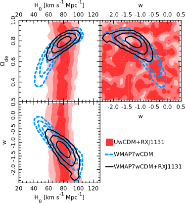
Figure 8.— RXJ1131$-$1231 marginalized posterior PDF for $H_{0}$, $\Omega_{\rm de}$ and $w$ in flat $w$CDM cosmological models. Contours/shades mark the 68.3%, 95.4%, 99.7% credible regions. The three sets of contours/shades correspond to three different prior/data set combinations. Shaded red: RXJ1131$-$1231 constraints given by the U$w$CDM prior; dashed blue: the prior provided by the WMAP7 data set alone; solid black: the joint constraints from combining WMAP7 and RXJ1131$-$1231.

9.2. Comparison between RXJ1131$-$1231 and B1608$+$656

How do the results of RXJ1131$-$1231 compare with that of B1608$+$656? We show in Figure 9 the overlay of the cosmological constraints of RXJ1131$-$1231 and B1608$+$656 in U$H_{0}$ (top panel) and U$w$CDM (bottom panel). To investigate the consistency of the two data sets, we need to consider their likelihood functions in the multi-dimensional cosmological parameter space: inconsistency is defined by insufficient overlap between the two likelihoods. We follow Marshall et al. (2006), and compute the Bayes Factor $F$ in favor of a single set of cosmological parameters and a simultaneous fit:

$$F=\frac{\langle L^{\rm R}L^{\rm B}\rangle}{\langle L^{\rm R}\rangle\langle L^{\rm B}\rangle},$$ (27)

where $L^{\rm R}$ and $L^{\rm B}$ are the likelihoods of the RXJ1131$-$1231 and B1608$+$656 data respectively, computed at each prior sample point. See the Appendix for the derivation of this result.

For the cosmology U$H_{0}$, the Bayes Factor is 3.2; for U$w$CDM, it takes the value 3.8. For comparison, with two one-dimensional Gaussian PDFs, $F$ takes the value of 1 when the two distributions overlap at their 2$\sigma$ points, and is about 3.6 when they overlap at their 1$\sigma$ point. From this we conclude that the results from RXJ1131$-$1231 and B1608$+$656 are consistent with each other. We do not detect any significant residual systematics given the current uncertainties in our measurements.

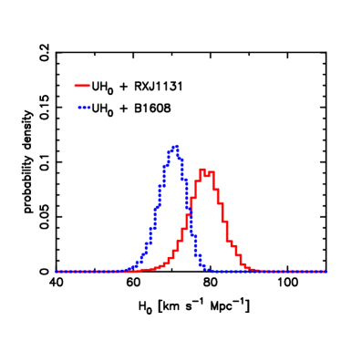
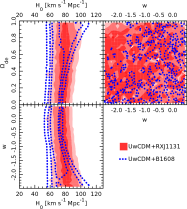
Figure 9.— Comparison of RXJ1131$-$1231 (solid red) with B1608$+$656 (dotted blue) in U$H_{0}$ (top) and U$w$CDM (bottom) cosmologies. The two distributions overlap within 2$\sigma$. The cosmological constraints from the two lenses are statistically consistent with each other: the ratio of the probability that the two lenses share global cosmological parameters to the probability that the lenses require independent cosmologies is 3.2 in U$H_{0}$ and 3.8 in U$w$CDM.

9.3. RXJ1131$-$1231 and B1608$+$656 in unison

Having shown that RXJ1131$-$1231 and B1608$+$656 yield consistent results with each other, we proceed to combine the results from these two lenses for cosmological inferences. In particular, we consider the constraints in the WMAP7$w$CDM and WMAP7o$\Lambda$CDM cosmologies in Table 2.

We show in Figure 10 the cosmological constraints from individual lenses in combination with WMAP7, and the combination of both lenses and WMAP7. By combining the two lenses, we tighten the constraints on $H_{0}$, $\Omega_{\rm de}$ and $\Omega_{\rm k}$. The precision on $w$ does not improve appreciably. With its low lens redshift, RXJ1131$-$1231 provide very little information to $w$ in addition to that obtained from B1608$+$656. In Table 4, we summarize the constraints from the two lenses.

WMAP7$w$CDM

 
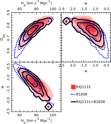
WMAP7o$\Lambda$CDM

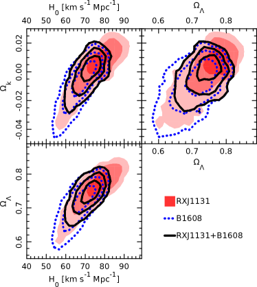
Figure 10.— Cosmological constraints from the combination of RXJ1131$-$1231 and B1608$+$656 assuming WMAP7$w$CDM (top) and WMAP7o$\Lambda$CDM (bottom) cosmologies. The combined posterior PDF is shown by the solid contours, the PDF for RXJ1131$-$1231 in combination with WMAP7 is the shaded contours, and the PDF for B1608$+$656 in combination with WMAP7 is the dotted contours. Contours/shades mark the 68.3%, 95.4%, 99.7% credible regions.

Table 4Cosmological constraints from RXJ1131$-$1231 and B1608$+$656 in combination with WMAP7

Cosmology	Parameter	Marginalized	Precision
		Value (68% CI)
	$H_{0}$	$75.2^{+4.4}_{-4.2}$	5.7%
$w$CDM	$\Omega_{\rm de}$	$0.76^{+0.02}_{-0.03}$	2.5%
	$w$	$-1.14^{+0.17}_{-0.20}$	18%
	$H_{0}$	$73.1^{+2.4}_{-3.6}$	4.0%
o$\Lambda$CDM	$\Omega_{\Lambda}$	$0.75^{+0.01}_{-0.02}$	1.9%
	$\Omega_{\rm k}$	$0.003^{+0.005}_{-0.006}$	0.6%

Notes. The $H_{0}$ values are in units of $\rm km\,s^{-1}\,Mpc^{-1}$. The “precision” in the fourth column is defined as half the 68% confidence interval, as a percentage of 75 for $H_{0}$, $1$ for $\Omega_{\rm de}$, $\Omega_{\Lambda}$, and $\Omega_{\rm k}$, and $-1.0$ for $w$.

9.4. Comparison of lenses and other cosmographic probes

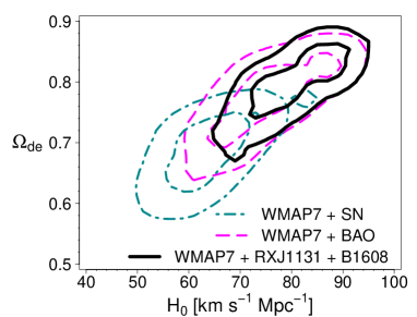
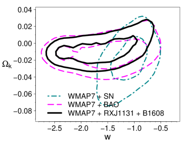
Figure 11.— Posterior PDF of $H_{0}$, $\Omega_{\rm de}$, $w$ and $\Omega_{\rm k}$ for SN (turquoise dot-dashed; Hicken et al. (2009)), BAO (magenta dashed; Percival et al. (2010)), time-delay lenses (black solid; this work) when each is combined with WMAP7 in an o$w$CDM cosmology. Contours mark the 68%, and 95% credible regions. Time-delay lenses are highly complementary to other probes, particularly the CMB and SN.

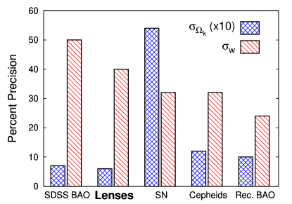
Figure 12.— Precision of cosmological constraints on $\Omega_{\rm k}$ and $w$ for five probes each in combination with WMAP in an o$w$CDM cosmology: SDSS BAO (Percival et al., 2010), the two time-delay lenses RXJ1131$-$1231 and B1608$+$656 (this work), SN (Suzuki et al., 2012), Cepheids (Riess et al., 2011), and reconstructed BAO (Mehta et al., 2012). Precision for $\Omega_{\rm k}$ and $w$ is defined as half the 68% CI as a percentage of 1 and $-1$, respectively.

How do the robust time-delay distances from the strong lenses compare to the distance measures of other probes? We show in Figure 11 a comparison of the cosmological constraints of the two lenses, Baryon Acoustic Oscillations (BAO; e.g., Percival et al., 2010; Blake et al., 2011; Mehta et al., 2012), and supernovae (SN; e.g., Hicken et al., 2009; Suzuki et al., 2012), when each is combined with WMAP7 in the o$w$CDM cosmology. The figures are qualitative since the samples for WMAP7 chain in the o$w$CDM cosmology are sparse and we have smoothed the contours after importance sampling. Nonetheless, we see that the sizes of the contours are comparable, suggesting that even a small sample of time-delay lenses is a powerful probe of cosmology. Both the lenses and BAO are strong in constraining the curvature of the Universe, while SN provides more information on the dark energy equation of state. Lenses are thus highly complementary to other cosmographic probes, particularly the CMB and SN (see also, e.g., Linder, 2011; Das & Linder, 2012). Each probe is consistent with flat $\Lambda$CDM: $\Omega_{\rm k}=0$ and $w=-1$ are within the 95% credible regions.

In Figure 12, we compare the precisions on $\Omega_{\rm k}$ and $w$ in o$w$CDM from the following cosmological probes in combination with WMAP: BAO from the Sloan Digital Sky Survey (SDSS) (Percival et al., 2010), our two time-delay lenses, SN from the Union 2.1 sample (Suzuki et al., 2012), the Cepheids distance ladder (Riess et al., 2011), and reconstructed BAO using the SDSS galaxies (Mehta et al., 2012). We note that the precisions on the Cepheids and the time-delay lenses are only approximates since the samples of WMAP7 are sparse in o$w$CDM due to the large parameter space. Nonetheless, the histogram plot shows that time-delay lenses are a valuable probe, especially in constraining the spatial curvature of the Universe.

10. Summary

We have performed a blind analysis of the time-delay lens RXJ1131$-$1231, modeling its high precision time delays from the COSMOGRAIL collaboration, deep HST imaging, newly measured lens velocity dispersion, and mass contribution from line-of-sight structures. The data sets were combined probabilistically in a joint analysis, via a comprehensive model of the lens system consisting of the light of the source AGN and its host galaxy, the light and mass of the lens galaxies, and structures along the line of sight characterized by external convergence and shear parameters. The resulting time-delay distance measurement for the lens allows us to infer cosmological constraints. From this study, we draw the following conclusions:

1. Our comprehensive lens model reproduces the global features of the HST image and the time delays. We quantify the uncertainty due to the deflector gravitational potential on the time-delay distance to be at the $4.6\%$ level.

2. Based on the external shear strength from the lens model and the overdensity of galaxy count around the lens, we obtained a PDF for the external convergence by ray tracing through the Millennium Simulation. This $\kappa_{\rm ext}$ PDF contributes to the uncertainty on $D_{\Delta t}$ also at the $4.6\%$ level.

3. Our robust time-delay distance measurement of $6\%$ takes into account all sources of known statistical and systematic uncertainty. We provide a fitting formula to describe the PDF of the time-delay distance that can be used to combine with any other independent cosmological probe.

4. The time-delay distance of RXJ1131$-$1231 is mostly sensitive to $H_{0}$, especially given the low redshift of the lens.

5. Assuming a flat $\Lambda$CDM with fixed $\Omega_{\Lambda}=0.73$ and uniform prior on $H_{0}$, our unblinded $H_{0}$ measurement from RXJ1131$-$1231 is $78.7^{+4.3}_{-4.5}\,\rm km\,s^{-1}\,Mpc^{-1}$.

6. The constraint on $H_{0}$ helps break parameter degeneracies in the CMB data. In combination with WMAP7 in $w$CDM, we find $H_{0}=80.0^{+5.8}_{-5.7}\,\rm km\,s^{-1}\,Mpc^{-1}$, $\Omega_{\rm de}=0.79\pm 0.03$, and $w=-1.25^{+0.17}_{-0.21}$. These are statistically consistent with the results from the gravitational lens B1608$+$656. There are no significant residual systematics detected in our method based on this combined analysis of the two systems.

7. By combining RXJ1131$-$1231, B1608$+$656 and WMAP7, we derive the following constraints: $H_{0}=75.2^{+4.4}_{-4.2}\,\rm km\,s^{-1}\,Mpc^{-1}$, $\Omega_{\rm de}=0.76^{+0.02}_{-0.03}$ and $w=-1.14^{+0.17}_{-0.20}$ in flat $w$CDM, and $H_{0}=73.1^{+2.4}_{-3.6}\,\rm km\,s^{-1}\,Mpc^{-1}$, $\Omega_{\Lambda}=0.75^{+0.01}_{-0.02}$ and $\Omega_{\rm k}=0.003^{+0.005}_{-0.006}$ in open $\Lambda$CDM.

8. Our measurement of the Hubble constant is completely independent of those based on the local distance ladder method (e.g., Riess et al., 2011; Freedman et al., 2012), providing an important consistency check of the standard cosmological model and of general relativity.

9. A comparison of the lenses and other cosmological probes that are each combined with WMAP7 shows that the constraints from the lenses are comparable in precision to various state-of-the-art probes. Lenses are particularly powerful in measuring the spatial curvature of the universe, and are complementary to other cosmological probes.

Thanks to the dedicated monitoring by the COSMOGRAIL (e.g., Vuissoz et al., 2008; Courbin et al., 2011; Tewes et al., 2012b, a) and Kochanek et al. (2006) collaborations, the number of lenses with accurate and precise time delays are increasing. Deep HST imaging for three of these lenses will be obtained in cycle 20 to allow accurate lens mass modeling that turns the delays into distances. Using the estimated uncertainties of the time-delay distances of the three lenses, we expect to measure $H_{0}$ from our assembled sample of five lenses (B1608$+$656, RXJ1131$-$1231, and the three cycle 20 lenses) to roughly $3.8\%$ in a $w$CDM cosmology if no significant residual systematics are detected. Current and upcoming telescopes and surveys including the Panoramic Survey Telescope & Rapid Response System, Hyper-Suprime Camera on the Subaru Telescope, and Dark Energy Survey expect to detect hundreds of AGN lenses with dozens of delays measured (Oguri & Marshall, 2010). Ultimately, the Large Synoptic Survey Telescope will discover thousands of time-delay lenses, painting a bright future for cosmography with gravitational lens time delays.

Appendix A Quantifying data set consistency via the Bayes Factor $B$

Marshall et al. (2006) invite us to consider the following two hypotheses: (1) $\mathsf{H}^{\rm global}$, in which the two lenses share a common set of cosmological parameters $\mbox{\boldmath{${{\pi}}$}}=\{H_{0},\Omega_{\rm de},w\}$, and (2) $\mathsf{H}^{\rm ind}$, in which each of the two lenses is provided with its own independent set of cosmological parameters, $\mbox{\boldmath{${{\pi}}$}}^{\rm R}=\{H_{0}^{\rm R},\Omega_{\rm de}^{\rm R},w^{\rm R}\}$ and $\mbox{\boldmath{${{\pi}}$}}^{\rm B}=\{H_{0}^{\rm B},\Omega_{\rm de}^{\rm B},w^{\rm B}\}$, with which to fit the data. Each set of parameters covers the same prior volume as in $\mathsf{H}^{\rm global}$. If the two data sets are highly inconsistent, only $\mathsf{H}^{\rm ind}$ will provide a good fit to both data sets in a joint analysis. The question is, do the data require $\mathsf{H}^{\rm ind}$, or is $\mathsf{H}^{\rm global}$ sufficient?

We quantify the answer to this question with the evidence ratio, or Bayes Factor, in favor of $\mathsf{H}^{\rm global}$:

$$F=\frac{P(\mbox{\boldmath{${d}$}}^{\rm R},\mbox{\boldmath{${d}$}}^{\rm B}|\mathsf{H}^{\rm global})}{P(\mbox{\boldmath{${d}$}}^{\rm R}|\mathsf{H}^{\rm ind})\,P(\mbox{\boldmath{${d}$}}^{\rm B}|\mathsf{H}^{\rm ind})}.$$ (A1)

where we have collectively denoted all the data sets of RXJ1131$-$1231 as $\mbox{\boldmath{${d}$}}^{\rm R}$ and of B1608$+$656 as $\mbox{\boldmath{${d}$}}^{\rm B}$. Each of the terms on the right-hand side of the above equation can be written in terms of a multi-dimensional integral over the cosmological parameters. For example, we have (starting with the simpler terms in the denominators)

$$P(\mbox{\boldmath{${d}$}}^{\rm R}|\mathsf{H}^{\rm ind})=\int{\rm d}^{3}\mbox{\boldmath{${{\pi}}$}}^{\rm R}\,P(\mbox{\boldmath{${d}$}}^{\rm R}|\mbox{\boldmath{${{\pi}}$}}^{\rm R},\mathsf{H}^{\rm ind})\,P(\mbox{\boldmath{${{\pi}}$}}^{\rm R}|\mathsf{H}^{\rm ind}),$$ (A2)

where $P(\mbox{\boldmath{${d}$}}^{\rm R}|\mbox{\boldmath{${{\pi}}$}}^{\rm R},\mathsf{H}^{\rm ind})$ is the likelihood of the RXJ1131$-$1231 data sets (the weights for the cosmological samples) that we denote by $L^{\rm R}$. Equation (A2) is then just the ensemble average of the samples’ likelihood values,

$$P(\mbox{\boldmath{${d}$}}^{\rm R}|\mathsf{H}^{\rm ind})=\langle L^{\rm R}\rangle.$$ (A3)

For $P(\mbox{\boldmath{${d}$}}^{\rm B}|\mathsf{H}^{\rm ind})$, we can rewrite the likelihood $P(\mbox{\boldmath{${d}$}}^{\rm B}|\mbox{\boldmath{${{\pi}}$}}^{\rm B},\mathsf{H}^{\rm ind})$ in terms of $D_{\Delta t}^{\rm B}$ to make use of $P(D_{\Delta t}^{\rm B}|\mbox{\boldmath{${d}$}}^{\rm B},\mathsf{H}^{\rm ind})$ given by Equation (35) of Suyu et al. (2010):

$$P(\mbox{\boldmath{${d}$}}^{\rm B}|\mbox{\boldmath{${{\pi}}$}}^{\rm B},\mathsf{H}^{\rm ind})=\frac{P(D_{\Delta t}^{\rm B}(\mbox{\boldmath{${{\pi}}$}}^{\rm B})|\mbox{\boldmath{${d}$}}^{\rm B},\mathsf{H}^{\rm ind})\,P(\mbox{\boldmath{${d}$}}^{\rm B}|\mathsf{H}^{\rm ind})}{P(D_{\Delta t}^{\rm B}|\mathsf{H}^{\rm ind})}.$$ (A4)

The ratio $Z^{\rm B}=P(\mbox{\boldmath{${d}$}}^{\rm B}|\mathsf{H}^{\rm ind})/P(D_{\Delta t}^{\rm B}|\mathsf{H}^{\rm ind})$ is a constant factor since the prior on $D_{\Delta t}^{\rm B}$ is uniform; thus, we obtain

$$P(\mbox{\boldmath{${d}$}}^{\rm B}|\mathsf{H}^{\rm ind})=Z^{\rm B}\langle L^{\rm B}\rangle,$$ (A5)

where $L^{\rm B}$ is given by the likelihood of the time-delay distance $P(D_{\Delta t}^{\rm B}(\mbox{\boldmath{${{\pi}}$}}^{\rm B})|\mbox{\boldmath{${d}$}}^{\rm B},\mathsf{H}^{\rm ind})$.

Finally, for the numerator in Equation (A1), we have

$$P(\mbox{\boldmath{${d}$}}^{\rm R},\mbox{\boldmath{${d}$}}^{\rm B}|\mathsf{H}^{\rm global}) = \int{\rm d}^{3}\mbox{\boldmath{${{\pi}}$}}\,P(\mbox{\boldmath{${d}$}}^{\rm R}|\mbox{\boldmath{${{\pi}}$}},\mathsf{H}^{\rm global})\,P(\mbox{\boldmath{${d}$}}^{\rm B}|\mbox{\boldmath{${{\pi}}$}},\mathsf{H}^{\rm global})\,P(\mbox{\boldmath{${{\pi}}$}}|\mathsf{H}^{\rm global})$$ (A6)

$$= Z^{\rm B}\langle L^{\rm R}L^{\rm B}\rangle,$$

where the constant $Z^{\rm B}$ is the same as that in $P(\mbox{\boldmath{${d}$}}^{\rm B}|\mathsf{H}^{\rm ind})$ since the parameterization of the cosmology for each independent lens is identical to that of the global cosmology (i.e., $\mbox{\boldmath{${{\pi}}$}}^{B}$ and ${{\pi}}$ are the same cosmological parameterization). Substituting Equations (A3), (A5), and (A6) into Equation (A1), we obtain

$$F=\frac{\langle L^{\rm R}L^{\rm B}\rangle}{\langle L^{\rm R}\rangle\langle L^{\rm B}\rangle},$$ (A7)

which can be readily computed given the values of $L^{\rm R}$ and $L^{\rm B}$ (the weights) that we have for each cosmological sample.

References

- Anderson & Bedin (2010) Anderson, J., & Bedin, L. R. 2010, PASP, 122, 1035
- Auger et al. (2008) Auger, M. W., Fassnacht, C. D., Wong, K. C., et al. 2008, ApJ, 673, 778
- Auger et al. (2010) Auger, M. W., Treu, T., Bolton, A. S., et al. 2010, ApJ, 724, 511
- Barden et al. (2005) Barden, M., Rix, H.-W., Somerville, R. S., et al. 2005, ApJ, 635, 959
- Barkana (1998) Barkana, R. 1998, ApJ, 502, 531
- Barnabè et al. (2011) Barnabè, M., Czoske, O., Koopmans, L. V. E., Treu, T., & Bolton, A. S. 2011, MNRAS, 415, 2215
- Barnabè et al. (2009) Barnabè, M., Czoske, O., Koopmans, L. V. E., et al. 2009, MNRAS, 399, 21
- Bertin & Arnouts (1996) Bertin, E., & Arnouts, S. 1996, A&AS, 117, 393
- Binney & Tremaine (1987) Binney, J., & Tremaine, S. 1987, Galactic dynamics (Princeton, NJ, Princeton University Press, 1987, 747 p.)
- Blake et al. (2011) Blake, C., Davis, T., Poole, G. B., et al. 2011, MNRAS, 415, 2892
- Blandford & Narayan (1992) Blandford, R. D., & Narayan, R. 1992, ARA&A, 30, 311
- Brewer & Lewis (2008) Brewer, B. J., & Lewis, G. F. 2008, MNRAS, 390, 39
- Chartas et al. (2009) Chartas, G., Kochanek, C. S., Dai, X., Poindexter, S., & Garmire, G. 2009, ApJ, 693, 174
- Claeskens et al. (2006) Claeskens, J.-F., Sluse, D., Riaud, P., & Surdej, J. 2006, A&A, 451, 865
- Coe & Moustakas (2009) Coe, D., & Moustakas, L. A. 2009, ApJ, 706, 45
- Conley et al. (2006) Conley, A., Goldhaber, G., Wang, L., et al. 2006, ApJ, 644, 1
- Courbin (2003) Courbin, F. 2003, e-prints (astro-ph/0304497)
- Courbin et al. (2011) Courbin, F., Chantry, V., Revaz, Y., et al. 2011, A&A, 536, A53
- Das & Linder (2012) Das, S., & Linder, E. V. 2012, ArXiv e-prints (1207.1105)
- Dunkley et al. (2005) Dunkley, J., Bucher, M., Ferreira, P. G., Moodley, K., & Skordis, C. 2005, MNRAS, 356, 925
- Dye et al. (2008) Dye, S., Evans, N. W., Belokurov, V., Warren, S. J., & Hewett, P. 2008, MNRAS, 388, 384
- Dye & Warren (2005) Dye, S., & Warren, S. J. 2005, ApJ, 623, 31
- Fadely et al. (2010) Fadely, R., Keeton, C. R., Nakajima, R., & Bernstein, G. M. 2010, ApJ, 711, 246
- Falco (2005) Falco, E. E. 2005, New Journal of Physics, 7, 200
- Fassnacht et al. (2006) Fassnacht, C. D., Gal, R. R., Lubin, L. M., et al. 2006, ApJ, 642, 30
- Fassnacht et al. (2011) Fassnacht, C. D., Koopmans, L. V. E., & Wong, K. C. 2011, MNRAS, 410, 2167
- Fassnacht et al. (2002) Fassnacht, C. D., Xanthopoulos, E., Koopmans, L. V. E., & Rusin, D. 2002, ApJ, 581, 823
- Freedman & Madore (2010) Freedman, W. L., & Madore, B. F. 2010, ARA&A, 48, 673
- Freedman et al. (2012) Freedman, W. L., Madore, B. F., Scowcroft, V., et al. 2012, ArXiv e-prints (1208.3281)
- Freedman & Turner (2003) Freedman, W. L., & Turner, M. S. 2003, Reviews of Modern Physics, 75, 1433
- Freedman et al. (2001) Freedman, W. L., Madore, B. F., Gibson, B. K., et al. 2001, ApJ, 553, 47
- Frieman et al. (2008) Frieman, J. A., Turner, M. S., & Huterer, D. 2008, ARA&A, 46, 385
- Gavazzi et al. (2007) Gavazzi, R., Treu, T., Rhodes, J. D., et al. 2007, ApJ, 667, 176
- George et al. (2012) George, M. R., Leauthaud, A., Bundy, K., et al. 2012, ArXiv e-prints (1205.4262)
- Guo et al. (2010) Guo, Q., White, S., Li, C., & Boylan-Kolchin, M. 2010, MNRAS, 404, 1111
- Halkola et al. (2008) Halkola, A., Hildebrandt, H., Schrabback, T., et al. 2008, A&A, 481, 65
- Harrison (1974) Harrison, E. R. 1974, ApJ, 191, L51
- Hernquist (1990) Hernquist, L. 1990, ApJ, 356, 359
- Hicken et al. (2009) Hicken, M., Wood-Vasey, W. M., Blondin, S., et al. 2009, ApJ, 700, 1097
- Hilbert et al. (2009) Hilbert, S., Hartlap, J., White, S. D. M., & Schneider, P. 2009, A&A, 499, 31
- Hilbert et al. (2007) Hilbert, S., White, S. D. M., Hartlap, J., & Schneider, P. 2007, MNRAS, 382, 121
- Humphrey & Buote (2010) Humphrey, P. J., & Buote, D. A. 2010, MNRAS, 403, 2143
- Jackson (2007) Jackson, N. 2007, Living Reviews in Relativity, 10, 4
- Jaffe (1983) Jaffe, W. 1983, MNRAS, 202, 995
- Keeton (2003) Keeton, C. R. 2003, ApJ, 584, 664
- Keeton & Zabludoff (2004) Keeton, C. R., & Zabludoff, A. I. 2004, ApJ, 612, 660
- Kochanek (2002) Kochanek, C. S. 2002, ApJ, 578, 25
- Kochanek et al. (2006) Kochanek, C. S., Morgan, N. D., Falco, E. E., et al. 2006, ApJ, 640, 47
- Komatsu et al. (2011) Komatsu, E., Smith, K. M., Dunkley, J., et al. 2011, ApJS, 192, 18
- Koopmans & Treu (2003) Koopmans, L. V. E., & Treu, T. 2003, ApJ, 583, 606
- Koopmans et al. (2009) Koopmans, L. V. E., Bolton, A., Treu, T., et al. 2009, ApJ, 703, L51
- Lehar et al. (1992) Lehar, J., Hewitt, J. N., Burke, B. F., & Roberts, D. H. 1992, ApJ, 384, 453
- Lewis & Bridle (2002) Lewis, A., & Bridle, S. 2002, Phys. Rev. D, 66, 103511
- Linder (2011) Linder, E. V. 2011, Phys. Rev. D, 84, 123529
- MacArthur et al. (2008) MacArthur, L. A., Ellis, R. S., Treu, T., et al. 2008, ApJ, 680, 70
- Magain et al. (1998) Magain, P., Courbin, F., & Sohy, S. 1998, ApJ, 494, 472
- Mantz et al. (2010) Mantz, A., Allen, S. W., Rapetti, D., & Ebeling, H. 2010, MNRAS, 406, 1759
- Marshall et al. (2006) Marshall, P., Rajguru, N., & Slosar, A. 2006, Phys. Rev. D, 73, 067302
- Marshall et al. (2007) Marshall, P. J., Treu, T., Melbourne, J., et al. 2007, ApJ, 671, 1196
- Massey et al. (2010) Massey, R., Stoughton, C., Leauthaud, A., et al. 2010, MNRAS, 401, 371
- Mehta et al. (2012) Mehta, K. T., Cuesta, A. J., Xu, X., Eisenstein, D. J., & Padmanabhan, N. 2012, ArXiv e-prints (1202.0092)
- Momcheva et al. (2006) Momcheva, I., Williams, K., Keeton, C., & Zabludoff, A. 2006, ApJ, 641, 169
- Morgan et al. (2006) Morgan, C. W., Kochanek, C. S., Morgan, N. D., & Falco, E. E. 2006, ApJ, 647, 874
- Mosquera & Kochanek (2011) Mosquera, A. M., & Kochanek, C. S. 2011, ApJ, 738, 96
- Newton et al. (2011) Newton, E. R., Marshall, P. J., Treu, T., et al. 2011, ApJ, 734, 104
- Oguri & Marshall (2010) Oguri, M., & Marshall, P. J. 2010, MNRAS, 405, 2579
- Oke et al. (1995) Oke, J. B., Cohen, J. G., Carr, M., et al. 1995, PASP, 107, 375
- Peebles (1993) Peebles, P. J. E. 1993, Principles of Physical Cosmology
- Percival et al. (2007) Percival, W. J., Cole, S., Eisenstein, D. J., et al. 2007, MNRAS, 381, 1053
- Percival et al. (2010) Percival, W. J., Reid, B. A., Eisenstein, D. J., et al. 2010, MNRAS, 401, 2148
- Refsdal (1964) Refsdal, S. 1964, MNRAS, 128, 307
- Refsdal (1966) —. 1966, MNRAS, 132, 101
- Reid et al. (2012) Reid, M. J., Braatz, J. A., Condon, J. J., et al. 2012, ArXiv e-prints (1207.7292)
- Riess et al. (2011) Riess, A. G., Macri, L., Casertano, S., et al. 2011, ApJ, 730, 119
- Schechter et al. (1997) Schechter, P. L., Bailyn, C. D., Barr, R., et al. 1997, ApJ, 475, L85
- Schneider et al. (1992) Schneider, P., Ehlers, J., & Falco, E. E. 1992, Gravitational Lenses, XIV, 560 pp. 112 figs.. Springer-Verlag Berlin Heidelberg New York.
- Schneider et al. (2006) Schneider, P., Kochanek, C. S., & Wambsganss, J. 2006, Gravitational Lensing: Strong, Weak and Micro (Springer)
- Sérsic (1968) Sérsic, J. L. 1968, Atlas de galaxias australes (Cordoba, Argentina: Observatorio Astronomico, 1968)
- Shectman et al. (1996) Shectman, S. A., Landy, S. D., Oemler, A., et al. 1996, ApJ, 470, 172
- Sluse et al. (2003) Sluse, D., Surdej, J., Claeskens, J.-F., et al. 2003, A&A, 406, L43
- Sonnenfeld et al. (2012) Sonnenfeld, A., Treu, T., Gavazzi, R., et al. 2012, ApJ, 752, 163
- Springel et al. (2005) Springel, V., White, S. D. M., Jenkins, A., et al. 2005, Nature, 435, 629
- Suyu (2012) Suyu, S. H. 2012, ArXiv e-prints (1202.0287)
- Suyu & Halkola (2010) Suyu, S. H., & Halkola, A. 2010, A&A, 524, A94
- Suyu et al. (2010) Suyu, S. H., Marshall, P. J., Auger, M. W., et al. 2010, ApJ, 711, 201
- Suyu et al. (2009) Suyu, S. H., Marshall, P. J., Blandford, R. D., et al. 2009, ApJ, 691, 277
- Suyu et al. (2006) Suyu, S. H., Marshall, P. J., Hobson, M. P., & Blandford, R. D. 2006, MNRAS, 371, 983
- Suyu et al. (2012) Suyu, S. H., Treu, T., Blandford, R. D., et al. 2012, ArXiv e-prints (1202.4459)
- Suzuki et al. (2012) Suzuki, N., Rubin, D., Lidman, C., et al. 2012, ApJ, 746, 85
- Tewes et al. (2012a) Tewes, M., Courbin, F., & Meylan, G. 2012a, ArXiv e-prints (1208.5598)
- Tewes et al. (2012b) Tewes, M., Courbin, F., Meylan, G., et al. 2012b, ArXiv e-prints (1208.6009)
- Treu (2010) Treu, T. 2010, ARA&A, 48, 87
- Treu & Koopmans (2002) Treu, T., & Koopmans, L. V. E. 2002, MNRAS, 337, L6
- Treu & Koopmans (2004) —. 2004, ApJ, 611, 739
- Valdes et al. (2004) Valdes, F., Gupta, R., Rose, J. A., Singh, H. P., & Bell, D. J. 2004, ApJS, 152, 251
- Vegetti & Koopmans (2009) Vegetti, S., & Koopmans, L. V. E. 2009, MNRAS, 392, 945
- Vegetti et al. (2010) Vegetti, S., Koopmans, L. V. E., Bolton, A., Treu, T., & Gavazzi, R. 2010, MNRAS, 408, 1969
- Vuissoz et al. (2008) Vuissoz, C., Courbin, F., Sluse, D., et al. 2008, A&A, 488, 481
- Weinberg et al. (2012) Weinberg, D. H., Mortonson, M. J., Eisenstein, D. J., et al. 2012, ArXiv e-prints (1201.2434)
- Williams et al. (2006) Williams, K. A., Momcheva, I., Keeton, C. R., Zabludoff, A. I., & Lehár, J. 2006, ApJ, 646, 85
- Witt et al. (2000) Witt, H. J., Mao, S., & Keeton, C. R. 2000, ApJ, 544, 98
- Wong et al. (2011) Wong, K. C., Keeton, C. R., Williams, K. A., Momcheva, I. G., & Zabludoff, A. I. 2011, ApJ, 726, 84
- Wucknitz (2002) Wucknitz, O. 2002, MNRAS, 332, 951
- Zabludoff & Mulchaey (1998) Zabludoff, A. I., & Mulchaey, J. S. 1998, ApJ, 496, 39