Wave polynomials, transmutations and Cauchy’s problem for the Klein-Gordon equation

Abstract

We prove a completeness result for a class of polynomial solutions of the wave equation called wave polynomials and construct generalized wave polynomials, solutions of the Klein-Gordon equation with a variable coefficient. Using the transmutation (transformation) operators and their recently discovered mapping properties we prove the completeness of the generalized wave polynomials and use them for an explicit construction of the solution of the Cauchy problem for the Klein-Gordon equation. Based on this result we develop a numerical method for solving the Cauchy problem and test its performance.

1 Introduction

Let $\Omega\subset\mathbb{C}$ be a simply connected domain. Due to the Runge approximation theorem any harmonic in $\Omega$ function can be approximated uniformly on any compact subset inside $\Omega$ by harmonic polynomials. The harmonic polynomials are linear combinations of the polynomials $\operatorname{Re}(z-z_{0})^{n}$ and $\operatorname{Im}(z-z_{0})^{n}$, $n=0,1,\ldots,$ where $z_{0}$ is an arbitrary point in $\Omega$ and $z$ is a complex variable. This fact reflects the completeness of the system of harmonic polynomials $\left\{\operatorname{Re}(z-z_{0})^{n},\ \operatorname{Im}(z-z_{0})^{n}\right\}_{n=0}^{\infty}$ in the space of all harmonic functions in $\Omega$ in the sense of the normal convergence.

Instead of the Laplace equation let us consider the wave equation

$$w_{xx}-w_{tt}=0$$ (1)

and instead of the complex imaginary unit let us introduce the hyperbolic imaginary unit: $j^{2}=1$. Let $z$ denote the hyperbolic variable $z=x+jt$ [22], [28]. Analogously to the elliptic case the system of polynomials

$$\big{\{}\operatorname{Re}(x+jt)^{n}\quad\text{and}\quad\operatorname{Im}(x+jt)^{n}\big{\}}_{n=0}^{\infty}$$ (2)

is an infinite system of solutions of the wave equation. Up to now, to our best knowledge, no corresponding completeness result has been obtained. We call the polynomials (2) and their finite linear combinations wave polynomials, and one of the first results of the present work is a Runge-type theorem establishing that any regular solution of (1) in a closed square $\overline{R}$ with the vertices $(\pm 2b,0)$ and $(0,\pm 2b)$, $b>0$ can be uniformly approximated on $\overline{R}$ by the wave polynomials. This theorem is auxiliary for obtaining a similar result for solutions of the Klein-Gordon equation with a variable coefficient

$$u_{xx}-u_{tt}-q(x)u=0$$ (3)

which we consider next. The construction of an infinite system of solutions similar to the wave polynomials was done in [19] with the aid of L. Bers’ results on pseudoanalytic formal powers [2] extended onto the hyperbolic situation. Similarly to the wave polynomials these generalized wave polynomials are components of formal powers, solutions of a corresponding hyperbolic Vekua equation which locally behave as powers of $z=x+jt$ but in general are not of course powers. Using recent results from [3] on mapping properties of transmutation operators we show that the generalized wave polynomials are images of the wave polynomials under the action of a transmutation operator. Due to the uniform boundedness of the transmutation operator and of its inverse several useful properties of the wave polynomials are preserved also in the case of their generalizations. In particular, the expansion theorem and the Runge-type theorem result to be valid.

All these observations lead to a new representation for the solution of the Cauchy problem for (3). It is based on the expansion of the Cauchy data into series in terms of a certain system of functions $\left\{\varphi_{k}\right\}_{k=0}^{\infty}$ which are introduced as recursive integrals and arise in the spectral parameter power series (SPPS) representation for solutions of Sturm-Liouville equations [14], [18]. In [16] a completeness of $\left\{\varphi_{k}\right\}_{k=0}^{\infty}$ in $L_{2}$ was proved. In [17] this result was obtained for the space of continuous and piecewise continuously differentiable functions. Here we show that the completeness of $\left\{\varphi_{k}\right\}_{k=0}^{\infty}$ in the space of continuous functions directly follows from the mapping properties of the transmutation operator and the Weierstrass approximation theorem. In [17] it was shown that several classical results from the theory of power series can be generalized onto the series in terms of the functions $\varphi_{k}$, including the Taylor formula. Here we present several new results on the approximation of continuous functions by linear combinations of functions $\varphi_{k}$. In particular, we show that the system of functions $\{\varphi_{k}\}_{k=0}^{\infty}$ in a real-valued case is a Tchebyshev system, prove a direct and an inverse approximation theorems and study algorithms for such approximation.

Using the results on the approximation by functions $\varphi_{k}$ we propose a numerical method for solving the Cauchy problem for (3) and illustrate its performance with several test examples. Once the Cauchy data are approximated by functions $\varphi_{k}$, the approximate solution of the Cauchy problem is written in a closed form. As for $t>0$ the approximate solution is an exact solution of equation (3) the only task consists in a good approximation of the Cauchy data. We show that in fact with relatively few functions $\varphi_{k}$ involved, a remarkable accuracy is achieved.

2 Wave polynomials

Let us consider the wave equation

$$\square w=0,\qquad\square:=\frac{\partial^{2}}{\partial x^{2}}-\frac{\partial^{2}}{\partial t^{2}}$$ (4)

and the following infinite family of its polynomial solutions

$$\big{\{}\operatorname{Re}(x+jt)^{n}\quad\text{and}\quad\operatorname{Im}(x+jt)^{n}\big{\}}_{n=0}^{\infty}$$ (5)

where $j$ is a hyperbolic imaginary unit, $j^{2}=1$.

It is easy to see that

$$\operatorname{Re}(x+jt)^{n}=\frac{1}{2}\big{(}(x+t)^{n}+(x-t)^{n}\big{)}\quad\text{and}\quad\operatorname{Im}(x+jt)^{n}=\frac{1}{2}\big{(}(x+t)^{n}-(x-t)^{n}\big{)}.$$ (6)

Let us reorder these polynomials as follows

$$p_{0}(x,t)=1\text{,\quad}p_{1}(x,t)=\operatorname{Re}(x+jt)=x\text{,\quad}p_{2}(x,t)=\operatorname{Im}(x+jt)=t\text{,}$$

$$p_{3}(x,t)=\operatorname{Re}(x+jt)^{2}=x^{2}+t^{2}\text{,\quad}p_{4}(x,t)=\operatorname{Im}(x+jt)^{2}=2xt\text{,\ldots.}$$

The obtained family of solutions of (4) will be called wave polynomials. It is convenient to write them also in the following form

$$p_{0}(x,t)=1\text{,\qquad}p_{m}(x,t)=\begin{cases}{\displaystyle\sum_{\text{even }k=0}^{\frac{m+1}{2}}\binom{\frac{m+1}{2}}{k}x^{\frac{m+1}{2}-k}t^{k},}&m\text{ odd},\\ {\displaystyle\sum_{\text{odd }k=1}^{\frac{m}{2}}\binom{\frac{m}{2}}{k}x^{\frac{m}{2}-k}t^{k},}&m\text{ even}.\end{cases}$$ (7)

Consider equation (4) together with the following Goursat conditions

$$w=\varphi(x)\text{ for }x-t=0\text{ and }w=\psi(x)\text{ for }x+t=0\quad(-b\leq x\leq b),$$

assuming additionally that $\varphi(0)=\psi(0)$. It is well known (see, e.g., [30, 4.1.1-9.]) that for $\varphi$ and $\psi$ belonging to $C^{2}[-b,b]$ the solution of the Goursat problem exists, is unique and has the form

$$w(x,t)=\varphi\Big{(}\frac{x+t}{2}\Big{)}+\psi\Big{(}\frac{x-t}{2}\Big{)}-\varphi(0).$$ (8)

Its domain of definition is a closed square $\overline{R}$ with the vertices $(\pm 2b,0)$ and $(0,\pm 2b)$.

Proposition 1

Let the boundary data $\varphi$ and $\psi$ be real-analytic functions with the corresponding power series expansions

$$\varphi(x)=\sum_{n=0}^{\infty}\alpha_{n}x^{n}\quad\text{and}\quad\psi(x)=\sum_{n=0}^{\infty}\beta_{n}x^{n},$$ (9)

uniformly convergent on $[-b,b]$ and satisfying necessary condition $\varphi(0)=\psi(0)$, i.e., $\alpha_{0}=\beta_{0}$. Then the unique solution of the Goursat problem has the form

$$w(x,t)=\alpha_{0}p_{0}(x,t)+\sum_{n=1}^{\infty}\frac{\alpha_{n}+\beta_{n}}{2^{n}}p_{2n-1}(x,t)+\sum_{n=1}^{\infty}\frac{\alpha_{n}-\beta_{n}}{2^{n}}p_{2n}(x,t)$$

where the series converge uniformly in $\overline{R}$.

Proof. From (6) we have

$$p_{2n-1}(x,t)=\frac{1}{2}\big{(}(x+t)^{n}+(x-t)^{n}\big{)}\quad\text{and}\quad p_{2n}(x,t)=\frac{1}{2}\big{(}(x+t)^{n}-(x-t)^{n}\big{)}$$

and hence

$$(x+t)^{n}=p_{2n-1}(x,t)+p_{2n}(x,t)\quad\text{and}\quad(x-t)^{n}=p_{2n-1}(x,t)-p_{2n}(x,t)\text{,\qquad}n=1,2,\ldots.$$ (10)

From (8) we obtain that the solution of the Goursat problem has the form

$$w(x,t)=\alpha_{0}+\sum_{n=1}^{\infty}\alpha_{n}\frac{(x+t)^{n}}{2^{n}}+\sum_{n=1}^{\infty}\beta_{n}\frac{(x-t)^{n}}{2^{n}}.$$

Substitution of the relations (10) gives us the equalities

$$\begin{split}w(x,t)&=\alpha_{0}+\sum_{n=1}^{\infty}\alpha_{n}\frac{p_{2n-1}(x,t)+p_{2n}(x,t)}{2^{n}}+\sum_{n=1}^{\infty}\beta_{n}\frac{p_{2n-1}(x,t)-p_{2n}(x,t)}{2^{n}}\\ &=\alpha_{0}p_{0}(x,t)+\sum_{n=1}^{\infty}\frac{\alpha_{n}+\beta_{n}}{2^{n}}p_{2n-1}(x,t)+\sum_{n=1}^{\infty}\frac{\alpha_{n}-\beta_{n}}{2^{n}}p_{2n}(x,t).\end{split}$$

 

Remark 2

From this proposition we obtain that the wave polynomials represent a basis in the linear space of solutions of the wave equation which admit a uniformly convergent in $\overline{R}$ power series expansion with the center in the origin. Indeed, consider any such solution of (4) in $\overline{R}$. Its values on the lines $x-t=0$ and $x+t=0$ admit uniformly convergent power series expansion of the form (9). According to the proposition the considered solution can be represented as a uniformly convergent series of the wave polynomials.

Let us prove the completeness of the wave polynomials in the linear space of regular solutions of the wave equation with respect to the maximum norm.

Theorem 3

Let $w\in C^{2}(\overline{R})$ be a solution of the wave equation (4) in $R$. Then there exists a sequence of wave polynomials $P_{N}=\sum_{n=0}^{N}a_{n}p_{n}$ uniformly convergent to $w$ in $\overline{R}$.

Proof. We need to prove that for any $\varepsilon>0$ there exist such a number $N$ and coefficients $a_{n}$, $n=0,1,\ldots N$ that $\left|w(x,t)-P_{N}(x,t)\right|<\varepsilon$ for any point $(x,t)\in\overline{R}$. Let $w=\varphi(x)$ for $x-t=0$ and $w=\psi(x)$ for $x+t=0$ ($-b\leq x\leq b$). We choose $\varepsilon>0$ and such $\varepsilon_{1,2}>0$ that $\varepsilon=2\varepsilon_{1}+2\varepsilon_{2}$. According to the Weierstrass theorem there exists such number $N$ and such polynomials $p_{1}$ and $p_{2}$ of order not greater than $N$ that $\left|\varphi(x)-p_{1}(x)\right|<\varepsilon_{1}$ and $\left|\psi(x)-p_{2}(x)\right|<\varepsilon_{2}$ ($-b\leq x\leq b$). We consider polynomials $q_{1}(x)=p_{1}(x)-p_{1}(0)+\varphi(0)$ and $q_{2}(x)=p_{2}(x)-p_{2}(0)+\psi(0)$ satisfying the condition $q_{1}(0)=q_{2}(0)=\varphi(0)$. Due to Proposition 1 the unique solution $\widetilde{w}$ of the Goursat problem with the boundary data $q_{1}$ and $q_{2}$ has the form $\widetilde{w}=P_{N}(x,t)$ where $P_{N}(x,t)=q_{1}\big{(}\frac{x+t}{2}\big{)}+q_{2}\big{(}\frac{x-t}{2}\big{)}-q_{1}(0)$. Consider

$$\begin{split}\left|w(x,t)-\widetilde{w}(x,t)\right|&=\left|w(x,t)-P_{N}(x,t)\right|\\ &\leq\Bigl{|}\varphi\Bigl{(}\frac{x+t}{2}\Bigr{)}-q_{1}\Bigl{(}\frac{x+t}{2}\Bigr{)}\Bigr{|}+\Bigl{|}\psi\Bigl{(}\frac{x-t}{2}\Bigr{)}-q_{2}\Bigl{(}\frac{x-t}{2}\Bigr{)}\Bigr{|}\\ &\leq\Bigl{|}\varphi\Bigl{(}\frac{x+t}{2}\Bigr{)}-p_{1}\Bigl{(}\frac{x+t}{2}\Bigr{)}\Bigr{|}+\bigl{|}\varphi(0)-p_{1}(0)\bigr{|}\\ &+\Bigl{|}\psi\Bigl{(}\frac{x-t}{2}\Bigr{)}-p_{2}\Bigl{(}\frac{x-t}{2}\Bigr{)}\Bigr{|}+\bigl{|}\psi(0)-p_{2}(0)\bigr{|}\leq 2\varepsilon_{1}+2\varepsilon_{2}=\varepsilon.\end{split}$$

 

3 Transmutation operators and their action on powers of the independent variable

3.1 Systems of recursive integrals

Let $f\in C^{2}(a,b)\cap C^{1}[a,b]$ be a complex valued function and $f(x)\neq 0$ for any $x\in[a,b]$. The interval $(a,b)$ is supposed to be finite. Let us consider the following auxiliary functions

$$\widetilde{X}^{(0)}(x) \equiv X^{(0)}(x)\equiv 1,$$ (11)

$$\widetilde{X}^{(n)}(x) =n\int_{x_{0}}^{x}\widetilde{X}^{(n-1)}(s)\left(f^{2}(s)\right)^{(-1)^{n-1}}\,\mathrm{d}s,$$ (12)

$$X^{(n)}(x) =n\int_{x_{0}}^{x}X^{(n-1)}(s)\left(f^{2}(s)\right)^{(-1)^{n}}\,\mathrm{d}s,$$ (13)

where $x_{0}$ is an arbitrary fixed point in $[a,b]$. We introduce the infinite system of functions $\left\{\varphi_{k}\right\}_{k=0}^{\infty}$ defined as follows

$$\varphi_{k}(x)=\begin{cases}f(x)X^{(k)}(x),&k\text{\ odd,}\\ f(x)\widetilde{X}^{(k)}(x),&k\text{\ even,}\end{cases}$$ (14)

where the definition of $X^{(k)}$ and $\widetilde{X}^{(k)}$ is given by (11)–(13) with $x_{0}$ being an arbitrary point of the interval $[a,b]$.

Example 4

Let $f\equiv 1$, $a=0$, $b=1$. Then it is easy to see that choosing $x_{0}=0$ we have $\varphi_{k}(x)=x^{k}$, $k\in\mathbb{N}_{0}$ where by $\mathbb{N}_{0}$ we denote the set of non-negative integers.

In [16] it was shown that the system $\left\{\varphi_{k}\right\}_{k=0}^{\infty}$ is complete in $L_{2}(a,b)$ and in [17] its completeness in the space of continuous and piecewise continuously differentiable functions with respect to the maximum norm was obtained and the corresponding series expansions in terms of the functions $\varphi_{k}$ were studied. The completeness in the space $C[a,b]$ is shown in the Proposition 27.

The system (14) is closely related to the notion of the $L$-basis introduced and studied in [8]. Here the letter $L$ corresponds to a linear ordinary differential operator. This becomes more transparent from the following result obtained in [14] (for additional details and simpler proof see [15] and [18]) establishing the relation of the system of functions $\left\{\varphi_{k}\right\}_{k=0}^{\infty}$ to Sturm-Liouville equations.

Theorem 5 ([14])

Let $q$ be a continuous complex valued function of an independent real variable $x\in[a,b],$ $\lambda$ be an arbitrary complex number. Suppose there exists a solution $f$ of the equation

$$f^{\prime\prime}-qf=0$$ (15)

on $(a,b)$ such that $f\in C^{2}[a,b]$ and $f\neq 0$ on $[a,b]$. Then the general solution of the equation

$$u^{\prime\prime}-qu=\lambda u$$ (16)

on $(a,b)$ has the form

$$u=c_{1}u_{1}+c_{2}u_{2}$$

where $c_{1}$ and $c_{2}$ are arbitrary complex constants,

$$u_{1}={\displaystyle\sum\limits_{k=0}^{\infty}}\frac{\lambda^{k}}{(2k)!}\varphi_{2k}\quad\quad\text{and}\quad\quad u_{2}={\displaystyle\sum\limits_{k=0}^{\infty}}\frac{\lambda^{k}}{(2k+1)!}\varphi_{2k+1}$$ (17)

and both series converge uniformly on $[a,b]$.

The solutions $u_{1}$ and $u_{2}$ satisfy the initial conditions

$$u_{1}(x_{0}) =f(x_{0}), u_{1}^{\prime}(x_{0}) =f^{\prime}(x_{0}),$$

$$u_{2}(x_{0}) =0, u_{2}^{\prime}(x_{0}) =1/f(x_{0}).$$

Together with the family of functions $\left\{\varphi_{k}\right\}_{k=0}^{\infty}$ we consider a dual system of recursive integrals defined by the following relations involving the “second half” of the formal powers (11)–(13),

$$\psi_{k}(x)=\begin{cases}\dfrac{\widetilde{X}^{(k)}(x)}{f(x)},&k\text{\ odd,}\\ \dfrac{X^{(k)}(x)}{f(x)},&k\text{\ even.}\end{cases}$$ (18)

3.2 Generalized derivatives and generalized Taylor series

In [17] a notion of the generalized derivative was introduced which alows one to extend the theory of power series onto the series in terms of the functions $\varphi_{k}$ (the formal power series). Here we slightly modify the definition introduced in [17]. This modification simplifies formulas involving the generalized derivatives and reflects a better understanding of the nature of the functions $\varphi_{k}$ and $\psi_{k}$ in the light of application of transmutation operators. We assume that the complex-valued function $f$ is continuous on $[a,b]$, $f(x)\neq 0$ for any $x\in[a,b]$ and $f(x_{0})=1$.

Definition 6

The generalized derivatives or the $f$-derivatives of a function $g$ are defined by the following relations whenever they make sense. The generalized derivative of a zero order coincides with the function $g$, $d_{0}^{f}[g](x)=g(x)$. The generalized derivatives of higher orders are defined as follows $d_{k}^{f}[g]=f^{(-1)^{k-1}}\frac{d}{dx}\left(f^{(-1)^{k}}d_{k-1}^{f}[g]\right)$, $k=1,2,\ldots$.

That is,

$$d_{k}^{f}[g]=\begin{cases}f\frac{d}{dx}\left(\frac{1}{f}d_{k-1}^{f}[g]\right),&k\ \text{ odd},\\ \frac{1}{f}\frac{d}{dx}\left(fd_{k-1}^{f}[g]\right),&k\ \text{ even}.\end{cases}$$

Remark 7

Let $f$ be a solution of (15) satisfying the conditions of Theorem 5. Then the corresponding differential operator can be factorized in the following way $L=\frac{d^{2}}{dx^{2}}-q(x)$ $=\frac{1}{f}\frac{d}{dx}\left(f^{2}\frac{d}{dx}\frac{1}{f}\ \cdot\right)$. This factorization sometimes is called the Polya factorization (see [11]).We see from it that $L=d_{2}^{f}$.

The generalized derivative $d_{1}^{f}=$ $f\frac{d}{dx}\left(\frac{1}{f}\ \cdot\right)$ coincides with the Darboux transformation (see, e.g., [26]).

Remark 8

It is easy to see that

$$d_{1}^{f}\varphi_{k}=k\psi_{k-1},\quad k=1,2,\ldots,$$

$$d_{2}^{f}\varphi_{k}=k(k-1)\varphi_{k-2},\quad k=2,3,\ldots.$$

and

$$d_{1}^{f}\varphi_{0}=d_{2}^{f}\varphi_{0}=d_{2}^{f}\varphi_{1}=0.$$

Remark 9

Consideration of the $1/f$-derivatives defined according to Definition 6 leads to the dual relations

$$d_{1}^{1/f}\psi_{k}=k\varphi_{k-1},\quad k=1,2,\ldots$$

and

$$d_{2}^{1/f}=f\frac{d}{dx}\left(\frac{1}{f^{2}}\frac{d}{dx}f\ \cdot\right)=\frac{d^{2}}{dx^{2}}-q_{D}(x)$$

where the potential $q_{D}$ is a superpartner of $q$ defined by the equality $q_{D}=-q+2\left(\frac{f^{\prime}}{f}\right)^{2}$ (see Subsection 3.3).

Definition 10

Functions of the form

$$P_{n}(x)=\sum\limits_{k=0}^{n}\alpha_{k}\varphi_{k}(x)$$ (19)

where $\alpha_{k}$, $k=0,1,\ldots,n$ are complex numbers are called $f$-polynomials of the order $n$.

In a complete similarity to the fact that the coefficients of a polynomial $\sum_{k=0}^{n}a_{k}(x-x_{0})^{k}$ can be expressed through its value and the values of its derivatives at the point $x_{0}$, the coefficients of an $f$-polynomial are determined by the values of $P_{n}$ and of its $f$-derivatives at $x_{0}$ (at the initial point of integration in (12), (13)). Indeed, a simple calculation using Remark 8 gives us the following result

$$\alpha_{k}=\frac{d_{k}^{f}[P_{n}](x_{0})}{k!}.$$

Let us consider a function $g$ possessing at the point $x_{0}$ the $f$-derivatives of all orders up to the order $n$. More precisely this means that the function $g$ is defined and possesses the $f$-derivatives of all orders up to the order $n-1$ in some segment $[a,b]$ containing the point $x_{0}$ and additionally there exists the $n$-th $f$-derivative of $g$ at the point $x_{0}$. In relation with the function $g$, we introduce an $f$-polynomial of the form (19) with the coefficients

$$\alpha_{k}=\frac{d_{k}^{f}[g](x_{0})}{k!}.$$

According to the previous observation, this $f$-polynomial together with its $f$-derivatives at $x_{0}$ up to the order $n$ take the same values as the function $g$ and its respective $f$-derivatives, $d_{k}^{f}[P_{n}](x_{0})=d_{k}^{f}[g](x_{0})$, $k=0,1,\ldots,n$. We are interested in estimating the difference between $P_{n}(x)$ and $g(x)$ for $x\neq x_{0}$.

Theorem 11 (Generalized Taylor theorem with the Peano form of the remainder term)

Let the function $g$ possesses at the point $x_{0}$ the $f$-derivatives of all orders up to the order $n$ and $f$ be a continuously differentiable function in a neighborhood of $x_{0}$. Then

$$g(x)=\sum_{k=0}^{n}\frac{d_{k}^{f}[g](x_{0})}{k!}\varphi_{k}(x)+o\big{(}(x-x_{0})^{n}\big{)}.$$

Proof. Consider the difference $r(x)=g(x)-P_{n}(x)$. We have

$$r(x_{0})=d_{1}^{f}[r](x_{0})=\cdots=d_{n}^{f}[r](x_{0})=0.$$ (20)

Let us prove by induction that if a function $r$ satisfies the conditions (20) or the conditions

$$r(x_{0})=d_{1}^{1/f}[r](x_{0})=\cdots=d_{n}^{1/f}[r](x_{0})=0,$$ (21)

then necessarily $r(x)=o\big{(}(x-x_{0})^{n}\big{)}$.

For $n=1$ this assertion has the form: if the function $r(x)$ possessing at $x_{0}$ the first $f$-derivative fulfills the conditions $r(x_{0})=d_{1}^{f}[r](x_{0})=0$ or possessing at $x_{0}$ the first $1/f$-derivative fulfills the conditions $r(x_{0})=d_{1}^{1/f}[r](x_{0})=0$ then $r(x)=o(x-x_{0})$. Its validity can be verified directly. In the first case we have

$$\lim_{x\rightarrow x_{0}}\frac{r(x)}{x-x_{0}}=f(x_{0})\lim_{x\rightarrow x_{0}}\frac{r(x)/f(x)}{x-x_{0}}=f(x_{0})\lim_{x\rightarrow x_{0}}\frac{\frac{r(x)}{f(x)}-\frac{r(x_{0})}{f(x_{0})}}{x-x_{0}}=0$$

due to the condition $d_{1}^{f}[r](x_{0})=0$, and in the second case the proof is completely similar.

Assume that the assertion is true for some $n\geq 1$. Due to the symmetry of (20) and (21) it is enough to prove that if for a function $r(x)$ possessing at $x_{0}$ the $f$-derivatives up to the order $n+1$ the following conditions are fulfilled $r(x_{0})=d_{1}^{f}[r](x_{0})=\cdots=d_{n+1}^{f}[r](x_{0})=0$ then $r(x)=o\big{(}(x-x_{0})^{n+1}\big{)}$. For this we observe that $r(x)$ fulfills the conditions (20) meanwhile $d_{1}^{f}[r]$ fulfills the conditions (21) and hence by the assumption we have $r(x)=o\big{(}(x-x_{0})^{n}\big{)}$ and $d_{1}^{f}[r](x)=o\big{(}(x-x_{0})^{n}\big{)}.$ Notice that by the mean value theorem

$$r(x)= r(x)-r(x_{0})=\left(\operatorname{Re}r^{\prime}(c_{1})+i\operatorname{Im}r^{\prime}(c_{2})\right)(x-x_{0})$$

$$= \left(\operatorname{Re}\Bigl{(}d_{1}^{f}[r](c_{1})+\frac{f^{\prime}(c_{1})}{f(c_{1})}r(c_{1})\Bigr{)}+i\operatorname{Im}\Bigl{(}d_{1}^{f}[r](c_{2})+\frac{f^{\prime}(c_{2})}{f(c_{2})}r(c_{2})\Bigr{)}\right)(x-x_{0}),$$

where $c_{1}$ and $c_{2}$ are located between $x_{0}$ and $x$. As $\left|c_{1,2}-x_{0}\right|<\left|x-x_{0}\right|$, then $d_{1}^{f}[r](c_{1,2})=o\bigl{(}(c_{1,2}-x_{0})^{n}\bigr{)}=o\bigl{(}(x-x_{0})^{n}\bigr{)}$ and $r(c_{1,2})=o\bigl{(}(c_{1,2}-x_{0})^{n}\bigr{)}=o\bigl{(}(x-x_{0})^{n}\bigr{)}$. Thus, we obtain $r(x)=o\bigl{(}(x-x_{0})^{n+1}\bigr{)}$.   

Under an additional condition that $f$ is real valued we obtain the following result by applying the reasoning from [17].

Theorem 12 (Generalized Taylor theorem with the Lagrange form of the remainder)

Let the real-valued function $g$ possesses on the segment $[x_{0},b]$ continuous $f$-derivatives of all orders up to the order $n$ and there exists a bounded $(n+1)$-th $f$-derivative of $g$ on $\left(x_{0},b\right)$. Let $f$ be a real-valued, continuously differentiable function in $[x_{0},b]$. Then for any $x\in[x_{0},b]$ there exists a number $c$ between $x_{0}$ and $x$ such that

$$g(x)=\sum_{k=0}^{n}\frac{d_{k}^{f}(g)(x_{0})}{k!}\varphi_{k}(x)+\frac{d_{n+1}^{f}(g)(c)}{(n+1)!}\varphi_{n+1}(x).$$

Proof. The proof is a simple adaptation of the proof from [17] according to the modified definition of generalized derivatives. All the steps and reasonings do not essentially change.   

Obviously, the classical Taylor theorem with the Lagrange form of the remainder term is a special case of theorem 12 when $f\equiv 1$.

3.3 Transmutation operators

We give a definition of a transmutation operator from [21] which is a modification of the definition given by Levitan [23] adapted to the purposes of the present work. Let $E$ be a linear topological space and $E_{1}$ its linear subspace (not necessarily closed). Let $A$ and $B$ be linear operators: $E_{1}\rightarrow E$.

Definition 13

A linear invertible operator $T$ defined on the whole $E$ such that $E_{1}$ is invariant under the action of $T$ is called a transmutation operator for the pair of operators $A$ and $B$ if it fulfills the following two conditions.

1. Both the operator $T$ and its inverse $T^{-1}$ are continuous in $E$;

2. The following operator equality is valid

   $$AT=TB$$ (22)

   or which is the same

   $$A=TBT^{-1}.$$

Very often in literature the transmutation operators are called the transformation operators. Here we keep the original term introduced by Delsarte and Lions [5]. Our main interest concerns the situation when $A=-\frac{d^{2}}{dx^{2}}+q(x)$, $B=-\frac{d^{2}}{dx^{2}}$,  and $q$ is a continuous complex-valued function. Hence for our purposes it will be sufficient to consider the functional space $E=C[a,b]$ with the topology of uniform convergence and its subspace $E_{1}$ consisting of functions from $C^{2}\left[a,b\right]$. One of the possibilities to introduce a transmutation operator on $E$ was considered by Lions [24] and later on in other references (see, e.g., [25]), and consists in constructing a Volterra integral operator corresponding to a midpoint of the segment of interest. As we begin with this transmutation operator it is convenient to consider a symmetric segment $[-b,b]$ and hence the functional space $E=C[-b,b]$. It is worth mentioning that other well known ways to construct the transmutation operators (see, e.g., [23], [38]) imply imposing initial conditions on the functions and consequently lead to transmutation operators satisfying (22) only on subclasses of $E_{1}$.

Thus, we consider the space $E=C[-b,b]$ and an operator of transmutation for the defined above $A$ and $B$ can be realized in the form (see, e.g., [23] and [25]) of a Volterra integral operator

$$Tu(x)=u(x)+\int_{-x}^{x}K(x,t)u(t)dt$$ (23)

where $K(x,t)$ is a unique solution of the Goursat problem

$$\left(\frac{\partial^{2}}{\partial x^{2}}-q(x)\right)K(x,t)=\frac{\partial^{2}}{\partial t^{2}}K(x,t),$$ (24)

$$K(x,x)=\frac{1}{2}\int_{0}^{x}q(s)ds,\qquad K(x,-x)=0.$$ (25)

In [3] the following mapping properties of the operator $T$ were proved.

Theorem 14 ([3])

Let $q$ be a continuous complex valued function of an independent real variable $x\in[-b,b]$ for which there exists a particular solution $f$ of (15) such that $f\in C^{2}[-b,b]$, $f\neq 0$ on $[-b,b]$ and normalized as $f(0)=1$. Denote $h:=f^{\prime}(0)\in\mathbb{C}$. Suppose $T$ is the operator defined by (23) where the kernel $K$ is a solution of the problem (24), (25) and $\varphi_{k}$, $k\in\mathbb{N}_{0}$ are functions defined by (14). Then the following equalities hold

$$\varphi_{k}=T[x^{k}],\quad\quad k\text{ odd}$$ (26)

and

$$\varphi_{k}-\frac{h}{k+1}\varphi_{k+1}=T[x^{k}],\quad\quad k\text{ even.}$$ (27)

Remark 15

Let $f$ be the solution of (15) satisfying the initial conditions

$$f(0)=1\quad\text{and}\quad f^{\prime}(0)=0.$$ (28)

If it does not vanish on $[-b,b]$ then from Theorem 14 we obtain that $\varphi_{k}=T[x^{k}]$ for any $k\in\mathbb{N}_{0}$. In general, of course there is no guaranty that the solution with such initial values would have no zero on $[-b,b]$, and hence the operator $T$ transmutes the powers of $x$ into $\varphi_{k}$ whose construction is based on the solution $f$ satisfying (28) only in some neighborhood of the origin.

In [3] it was shown that given a system of functions $\left\{\varphi_{k}\right\}_{k=0}^{\infty}$ defined by (14) where $f$ is any particular solution of (15) such that $f\in C^{2}[-b,b]$, $f\neq 0$ on $[-b,b]$ and $f(0)=1$, $f^{\prime}(0)=h\in\mathbb{C}$, the operator $T$ can be modified in such a way that the new transmutation operator will map $x^{k}$ to $\varphi_{k}$ for any $k\in\mathbb{N}_{0}$.

Theorem 16 ([3], [20])

Under the conditions of Theorem 14 the operator

$$\mathbf{T}u(x)=u(x)+\int_{-x}^{x}\mathbf{K}(x,t;h)u(t)dt$$ (29)

with the kernel defined by

$$\mathbf{K}(x,t;h)=\frac{h}{2}+K(x,t)+\frac{h}{2}\int_{t}^{x}\left(K(x,s)-K(x,-s)\right)ds$$ (30)

transforms $x^{k}$ into $\varphi_{k}(x)$ for any $k\in\mathbb{N}_{0}$ and

$$\left(-\frac{d^{2}}{dx^{2}}+q(x)\right)\mathbf{T}[u]=\mathbf{T}\left[-\frac{d^{2}}{dx^{2}}(u)\right]$$ (31)

for any $u\in C^{2}[-b,b]$.

Moreover, if the potential $q\in C^{1}[-b,b]$, then the kernel $\mathbf{K}(x,t;h)$ is a unique solution of the Goursat problem

$$\left(\frac{\partial^{2}}{\partial x^{2}}-q(x)\right)\mathbf{K}(x,t;h)=\frac{\partial^{2}}{\partial t^{2}}\mathbf{K}(x,t;h),$$ (32)

$$\mathbf{K}(x,x;h)=\frac{h}{2}+\frac{1}{2}\int_{0}^{x}q(s)\,ds,\qquad\mathbf{K}(x,-x;h)=\frac{h}{2}.$$ (33)

This theorem was proved in [3] under an additional assumption that the potential $q$ must be continuously differentiable, and in [20] it was shown that this assumption was superfluous due to new observed relations (38), (39) given below between the transmutations for Darboux transformed Schrödinger operators. The last statement of this theorem was proved in [20], also the interested reader may find in [20] necessary changes regarding the case when $q\in C[-b,b]$. For brevity, we omit these details in the present article.

In the following sections we use both the transmutation operator $\mathbf{T}$ and its inverse $\mathbf{T}^{-1}$, and the norms of these operators appear in many estimates. Hence it is natural to obtain convenient estimates for the norms. Remind that in [20] it was mentioned that to define the transmutation operator $\mathbf{T}$, we need to know its integral kernel in the domain $0\leq|t|\leq|x|\leq b$. But the Goursat problem (32)–(33) is also well-posed and allows to determine the kernel $\mathbf{K}(x,t;h)$ in the domain $0\leq|x|\leq|t|\leq b$. Thus we may assume that the integral kernel $\mathbf{K}(x,t;h)$ is known in the square $|x|\leq b$, $|t|\leq b$. In such case, there is a simple representation of the inverse operator $\mathbf{T}^{-1}$.

Theorem 17 ([20])

The inverse operator $\mathbf{T}^{-1}$ can be represented as the Volterra integral operator

$$\mathbf{T}^{-1}u(x)=u(x)-\int_{-x}^{x}\mathbf{K}(t,x;h)u(t)\,dt.$$ (34)

Both $\mathbf{T}$ and $\mathbf{T}^{-1}$ are obviously bounded as operators from $C[-b,b]$ to itself. The estimates for their norms depend on the estimates for the integral kernels, e.g., for $\left\|\mathbf{T}\right\|$ we have $\left\|\mathbf{T}\right\|\leq 1+2b\max\left|\mathbf{K}(x,t;h)\right|$. Some estimates for the integral kernel $K(x,t)$ can be found in [25]. From them corresponding estimates for the kernel $\mathbf{K}(x,t;h)$ can be obtained using (30). However, the growth with the increase of the interval of mentioned estimates is immensely fast even for the simplest potentials. We adapt the general method of successive approximations for solving Goursat problems (see, e.g. [39]) to obtain better estimates for the kernel $\mathbf{K}(x,t;h)$.

Proposition 18

Let $q$ be a continuous complex valued function of an independent real variable $x\in[-b,b]$. Then the kernel $\mathbf{K}(x,t;h)$ in the square $|x|\leq b$, $|t|\leq b$ satisfies the following estimate

$$|\mathbf{K}(x,t;h)|\leq\frac{|h|}{2}I_{0}\big{(}\sqrt{c|x^{2}-t^{2}|}\big{)}+\frac{1}{2}\frac{\sqrt{c|x^{2}-t^{2}|}I_{1}\big{(}\sqrt{c|x^{2}-t^{2}|}\big{)}}{|x-t|},$$ (35)

where $c=\max_{[-b,b]}|q(x)|$ and $I_{0}$ and $I_{1}$ are modified Bessel functions of the first kind.

Remark 19

Note that for the case of operator $\partial^{2}-c$ with constant potential $c>0$ and $h>0$ the exact kernel of transmutation operator in the domain $0\leq t\leq x\leq b$ coincides with the right-hand side of (35), see [3].

Proof. The proof follows the proof from [39]. First, we introduce the function $H(u,v):=\mathbf{K}(u+v,u-v;h)$. It satisfies the Goursat problem (see [20])

$$\frac{\partial^{2}H(u,v)}{\partial u\,\partial v}=q(u+v)H(u,v),$$ (36)

$$H(u,0)=\frac{h}{2}+\frac{1}{2}\int_{0}^{u}q(s)\,ds,\qquad H(0,v)=\frac{h}{2}$$ (37)

in the domain $|u|+|v|\leq b$. It is worth mentioning that despite the kernel $\mathbf{K}(x,t;h)$ is not the classical solution of the problem (32)–(33) in the case when $q\in C[-b,b]$, nevertheless the function $H(u,v)$ is a classical solution of the problem (36)–(37), see [20]. Define $G:=\frac{\partial H}{\partial u}$. Then the Goursat problem (36)–(37) is equivalent to the system of integral equations

$$\begin{cases}H(u,v)=\frac{h}{2}+\int_{0}^{u}G(u^{\prime},v)\,du^{\prime}\\ G(u,v)=\frac{1}{2}q(u)+\int_{0}^{v}q(u+v^{\prime})H(u,v^{\prime})\,dv^{\prime}.\end{cases}$$

Applying the successive approximations method for this system, we obtain

$$|H(u,v)|\leq\frac{|h|}{2}\sum_{k=0}^{\infty}\frac{c^{k}|uv|^{k}}{k!k!}+\frac{1}{2}\sum_{k=0}^{\infty}\frac{c^{k+1}|u|^{k+1}|v|^{k}}{(k+1)!k!},$$

which coincides with (35).   

Since the function $I_{1}(x)/x$ is monotone increasing for $x>0$, we obtain

$$\frac{\sqrt{c|x^{2}-t^{2}|}I_{1}\big{(}\sqrt{c|x^{2}-t^{2}|}\big{)}}{|x-t|}=c|x+t|\frac{I_{1}\big{(}\sqrt{c|x^{2}-t^{2}|}\big{)}}{\sqrt{c|x^{2}-t^{2}|}}\leq 2bc\frac{I_{1}(b\sqrt{c})}{b\sqrt{c}}=2\sqrt{c}I_{1}(b\sqrt{c})$$

for $|x|\leq b$ and $|t|\leq b$, and the following estimate for the norms of transmutation operator and of its inverse immediately follows from Proposition 18.

Corollary 20

The following estimate holds

$$\max\big{\{}\|\mathbf{T}\|,\|\mathbf{T}^{-1}\|\big{\}}\leq 1+b\left(|h|I_{0}(b\sqrt{c})+2\sqrt{c}I_{1}(b\sqrt{c})\right),$$

where $c=\max_{[-b,b]}|q(x)|$ and $I_{0}$ and $I_{1}$ are modified Bessel functions of the first kind.

Together with the operator $\frac{d^{2}}{dx^{2}}-q(x)$ let us consider a Darboux associated operator $\frac{d^{2}}{dx^{2}}-q_{D}(x)$ with the potential defined by the equality $q_{D}=-q+2\left(\frac{f^{\prime}}{f}\right)^{2}$ where $f\in C^{2}[-b,b]$ is a solution of (15), $f\neq 0$ on $[-b,b]$, $f(0)=1$ and $h=f^{\prime}(0)\in\mathbb{C}$. In [20] explicit formulas were obtained for the kernel $\mathbf{K}_{D}(x,t;-h)$ in terms of $\mathbf{K}(x,t;h)$, where $\mathbf{K}_{D}(x,t;-h)$ is the integral kernel of the transmutation operator $\mathbf{T}_{D}$ which satisfies the equality

$$\left(-\frac{d^{2}}{dx^{2}}+q_{D}(x)\right)\mathbf{T}_{D}[u]=\mathbf{T}_{D}\left[-\frac{d^{2}}{dx^{2}}(u)\right]$$

for any $u\in C^{2}[-b,b]$ and transforms $x^{k}$ into the functions $\psi_{k}(x)$, $k\in\mathbb{N}_{0}$ defined by the relations (18). Note that $\psi_{0}$ is obviously a solution of $\left(-\frac{d^{2}}{dx^{2}}+q_{D}(x)\right)\psi_{0}=0$ with the initial values $\psi_{0}(0)=1$ and $\psi_{0}^{\prime}(0)=-h$.

The operator $\mathbf{T}_{D}$ has the form [20]

$$\mathbf{T}_{D}[u](x)=u(x)+\int_{-x}^{x}\mathbf{K}_{D}(x,t;-h)u(t)\,dt,$$

with the kernel

$$\mathbf{K}_{D}(x,t;-h)=-\frac{1}{f(x)}\bigg{(}\int_{-t}^{x}\partial_{t}\mathbf{K}(s,t;h)f(s)\,ds+\frac{h}{2}f(-t)\bigg{)},$$

and the following operator equalities hold on $C^{1}[-b,b]$:

$$\frac{d}{dx}f\mathbf{T}_{D} =f\mathbf{T}\frac{d}{dx}$$ (38)

$$\frac{d}{dx}\frac{1}{f}\mathbf{T} =\frac{1}{f}\mathbf{T}_{D}\frac{d}{dx}.$$ (39)

These commutation equalities involving the operators of transmutation and derivatives together with the property of the transmutation operators that if $u\in C^{1}[-b,b]$ then $\mathbf{T}^{-1}u\in C^{1}[-b,b]$, see Theorem 17, lead to the following useful statement.

Proposition 21 ([21])

Let $u\in C^{n}[-b,b]$ and $g=\mathbf{T}u$. Then there exist the first $n$ $f$-derivatives of $g$ on $[-b,b]$, and the following equalities hold for $0\leq k\leq n$

$$d_{k}^{f}(g)=\mathbf{T}_{D}u^{(k)},\qquad k\text{ odd},$$

and

$$d_{k}^{f}(g)=\mathbf{T}u^{(k)},\qquad k\text{ even}.$$

The inverse statement, i.e., if there exist the first $n$ $f$-derivatives of $g$ on $[-b,b]$, then $u=\mathbf{T}^{-1}g\in C^{n}[-b,b]$ is also true.

4 Generalized wave polynomials

Let us consider the following Klein-Gordon equation with a position dependent mass

$$\left(\frac{\partial^{2}}{\partial x^{2}}-q(x)\right)u(x,t)=\frac{\partial^{2}}{\partial t^{2}}u(x,t)$$ (40)

where we assume that $q:[-b,b]\rightarrow\mathbb{C}$ and $q\in C[-b,b]$. Suppose there exists a particular solution $f$ of equation (15) such that $f\in C^{2}[-b,b]$ and $f\neq 0$ on $[-b,b]$. We normalize it as $f(0)=1$ and set $h:=f^{\prime}(0)$.

Consider the system of functions $\left\{\varphi_{k}\right\}_{k=0}^{\infty}$ defined by (14) with $x_{0}=0$. Then due to Theorem 16, $\varphi_{k}(x)=$ $\mathbf{T}x^{k}$ for any $k\in\mathbb{N}_{0}$ and due to (7) we obtain that the functions

$$u_{0}=f(x)\text{,\qquad}u_{m}(x,t)=\begin{cases}{\displaystyle\sum_{\text{even }k=0}^{\frac{m+1}{2}}\binom{\frac{m+1}{2}}{k}\varphi_{\frac{m+1}{2}-k}(x)t^{k},}&m\text{ odd},\\ {\displaystyle\sum_{\text{odd }k=1}^{\frac{m}{2}}\binom{\frac{m}{2}}{k}\varphi_{\frac{m}{2}-k}(x)t^{k},}&m\text{ even},\end{cases}$$ (41)

are solutions of (40) for any $-b<x<b$ and $-\infty<t<\infty$. Indeed, we have that

$$u_{m}=\mathbf{T}p_{m}\quad\text{for every }m\in\mathbb{N}_{0}\text{.}$$ (42)

Moreover, the functions $u_{m}$ arise also as scalar (real, when $f$ is real valued) parts of hyperbolic pseudoanalytic formal powers corresponding to the generating pair $(f,j/f)$ where j is a hyperbolic imaginary unit, $j^{2}=1$ (see [19], [15]).

Equalities (42) together with the completeness of the wave polynomials (Theorem 3) and the boundedness of $\mathbf{T}$ and $\mathbf{T}^{-1}$ imply the completeness of the generalized wave polynomials $u_{m}$ in the linear space of regular solutions of (40).

Theorem 22

Let $u\in C^{2}(\overline{\mathbf{R}})$ be a solution of (40) in $\mathbf{R}$ where $\mathbf{R}$ is a square with the vertices $(\pm b,0)$ and $(0,\pm b)$. Then there exists a sequence of generalized wave polynomials $U_{N}=\sum_{n=0}^{N}a_{n}u_{n}$ uniformly convergent to $u$ in $\overline{\mathbf{R}}$.

Proof. We have that $u=$ $\mathbf{T}w$ where $w$ is a $C^{2}$-solution of (4) and due to Theorem 3 for any $\varepsilon_{1}>0$ there exists a wave polynomial $P_{N}$ such that $\max_{\overline{\mathbf{R}}}\left|w-P_{N}\right|<\varepsilon_{1}$. Thus, $\max_{\overline{\mathbf{R}}}\left|u-\mathbf{T}P_{N}\right|=\max_{\overline{\mathbf{R}}}\left|\mathbf{T}w-\mathbf{T}P_{N}\right|\leq\varepsilon_{1}C=\varepsilon$. Here the constant $C$ depends only on the kernel $\mathbf{K}(x,t;h)$.   

Remark 23

When $t=0$ the following relations are valid

$$u_{m}(x,0)=\begin{cases}\varphi_{\frac{m+1}{2}}(x),&m\text{ odd}\\ 0,&m\text{ even}\end{cases}$$

and

$$\frac{\partial u_{m}(x,0)}{\partial t}=\begin{cases}0,&m\text{ odd}\\ \frac{m}{2}\,\varphi_{\frac{m}{2}-1}(x),&m\text{ even}.\end{cases}$$

These relations follow directly from the definition (41). One can write them also as follows

$$u_{2n-1}(x,0)=\varphi_{n}(x),\qquad u_{2n}(x,0)=0,$$

and

$$\frac{\partial u_{2n-1}(x,0)}{\partial t}=0,\qquad\frac{\partial u_{2n}(x,0)}{\partial t}=n\varphi_{n-1}(x),\qquad\text{for }n=1,2,\ldots.$$

For $u_{0}$ we have

$$u_{0}(x,0)=f(x)=\varphi_{0}(x)\qquad\text{and}\qquad\frac{\partial u_{0}(x,0)}{\partial t}=0.$$

5 Solution of the Cauchy problem

Consider the following initial value problem

$$\square u-q(x)u=0,\qquad-b\leq x\leq b,\quad t\geq 0$$ (43)

$$u(x,0)=g(x),\quad u_{t}(x,0)=h(x)$$ (44)

which for $q\in C[-b,b]$, $g\in C^{2}[-b,b]$, $h\in C^{1}[-b,b]$ possesses a unique solution (see, e.g., [39, Sect. 15.4]) in the triangle with the vertices $(\pm b,0)$ and $(0,b)$ (see illustration). For the convenience, later in this article we denote this triangle by the symbol $\blacktriangle$. We assume that $q$ satisfies the conditions of Theorem 14 and begin with the additional assumption that the functions $g$ and $h$ admit uniformly convergent series expansions in terms of the functions $\varphi_{k}$,

$$g(x)=\sum\limits_{k=0}^{\infty}\alpha_{k}\varphi_{k}(x)\qquad\text{and}\qquad h(x)=\sum\limits_{k=0}^{\infty}\beta_{k}\varphi_{k}(x).$$ (45)

We look for a solution of the problem (43), (44) in the form

$$u(x,t)=\sum\limits_{n=0}^{\infty}a_{n}u_{n}(x,t).$$ (46)

Then we have (see Remark 23)

$$u(x,0)=a_{0}\varphi_{0}(x)+\sum\limits_{n=1}^{\infty}a_{2n-1}u_{2n-1}(x,0)=a_{0}\varphi_{0}(x)+\sum\limits_{n=1}^{\infty}a_{2n-1}\varphi_{n}(x)$$

and

$$u_{t}(x,0)=\sum\limits_{n=1}^{\infty}a_{2n}\frac{\partial u_{2n}(x,0)}{\partial t}=\sum\limits_{n=1}^{\infty}a_{2n}n\varphi_{n-1}(x)=\sum\limits_{k=0}^{\infty}a_{2(k+1)}(k+1)\varphi_{k}(x).$$

Thus, if a solution of the problem (43), (44) in the form (46) exists, the expansion coefficients are obtained directly from the coefficients in the expansions (45) as follows

$$a_{0}=\alpha_{0}\text{,\quad}a_{2n-1}=\alpha_{n}\text{,\quad}n=1,2,\ldots\text{\qquad and \quad}a_{2(n+1)}=\frac{\beta_{n}}{n+1}\text{,\qquad}n=0,1,2,\ldots\text{.}$$ (47)

The following natural questions arise. Under which conditions given functions $g$ and $h$ are representable in the form (45) and whether such series expansion is unique? Can one guarantee the uniform convergence of the series (46) and that of its first and second derivatives in a domain of interest? In what follows we address these questions and show that the described scheme also leads to a powerful numerical technique for solving the initial value problems for equation (43).

Proposition 24

A continuous complex-valued function $g$ defined on $[-b,b]$ admits a series expansion of the form $g(x)=\sum_{k=0}^{\infty}\alpha_{k}\varphi_{k}(x)$ uniformly convergent on $[-b,b]$ if and only if there exists a complex-valued function $\widetilde{g}$ defined on $[-b,b]$ such that $g=\mathbf{T}\widetilde{g}$, $\widetilde{g}(x)=\sum_{k=0}^{\infty}\alpha_{k}x^{k}$ and the power series converges uniformly on $[-b,b]$. The expansion coefficients are uniquely defined by the equalities

$$\alpha_{k}=\frac{d_{k}^{f}(g)(0)}{k!}=\frac{\widetilde{g}^{\left(k\right)}(0)}{k!}.$$ (48)

Proof. The proof of the representability of $g$ in the form of a uniformly convergent series $\sum_{k=0}^{\infty}\alpha_{k}\varphi_{k}(x)$ follows from the uniform boundedness of the Volterra integral operators $\mathbf{T}$ and $\mathbf{T}^{-1}$. The linearity of these integral operators together with the fact that $\mathbf{T}\left[x^{k}\right]=\varphi_{k}$ (Theorem 16) gives us the equality between the coefficients of the corresponding series expansions of $g$ and $\widetilde{g}$. The equality $d_{k}^{f}(g)(0)=\widetilde{g}^{\left(k\right)}(0)$, $k=0,1,\ldots$ is a consequence of Proposition 21 and of the observation that at the origin $\mathbf{T}\left[u\right](0)=\mathbf{T}_{D}\left[u\right](0)=u(0)$ for any continuous function $u$.   

Proposition 25

Suppose that $g\in C[-b,b]$ and for any $k\in\mathbb{N}$ and $x\in(-b,b)$ there exists the generalized derivative $d_{k}^{f}(g)(x)$ such that for any $[-a,a]\subset(-b,b)$ the inequality holds

$$\left|d_{k}^{f}(g)\right|\leq C(a;k)\frac{k!}{b^{k}}$$

where the constants $C(a;k)$ do not depend on $x$ and the sequence $C(a;k)$ is of a subexponential growth ($\overline{\lim}\sqrt[k]{C(a;k)}\leq 1$). Then on $(-b,b)$   the function $g$ admits a normally convergent generalized Taylor series expansion

$$g(x)=\sum\limits_{k=0}^{\infty}\alpha_{k}\varphi_{k}(x)$$ (49)

and $\alpha_{k}=d_{k}^{f}(g)(0)/k!$.

Proof. Under the conditions of the proposition consider $\widetilde{g}=\mathbf{T}^{-1}g$. From Proposition 21 we have that $\widetilde{g}\in C^{\infty}(-b,b)$ and

$$\left|\widetilde{g}^{\left(k\right)}\right|\leq M\,C(a;k)\frac{k!}{b^{k}}$$

where $M=\max\left\{\left\|\mathbf{T}^{-1}\right\|,\,\left\|\mathbf{T}_{D}^{-1}\right\|\right\}$. Indeed, considering, e.g., an even $k$ we obtain $\left|\widetilde{g}^{\left(k\right)}\right|=\left|\mathbf{T}^{-1}d_{k}^{f}(g)\right|\leq\left\|\mathbf{T}^{-1}\right\|\max\left|d_{k}^{f}(g)\right|\leq\left\|\mathbf{T}^{-1}\right\|C(a;k)\frac{k!}{b^{k}}$ and analogously for an odd $k$.

From this we obtain that $\widetilde{g}$ admits on $(-b,b)$ a normally convergent Taylor series expansion of the form $\widetilde{g}(x)=\sum_{k=0}^{\infty}\alpha_{k}x^{k}$ and due to Proposition 24, $g$ admits a normally convergent generalized Taylor series expansion (49).   

Proposition 26

Let the initial data $g$ and $h$ admit uniformly convergent series expansions of the form (45) on $[-b,b]$. Then the unique (classical) solution of the Cauchy problem (43), (44) in $\blacktriangle$ has the form (46) which is uniformly convergent in $\blacktriangle$. The expansion coefficients are defined by (47).

Proof. As was previously shown if the series (46) together with the series corresponding to the first and second partial derivatives are normally convergent it satisfies equation (43) as well as the conditions (44). Thus, it remains to prove the uniform convergence of the involved series.

Using (42) we have $\left|u_{n}\right|\leq\left\|\mathbf{T}\right\|\cdot\max\left|p_{n}\right|$, and from (6) we obtain

$$\left|u_{n}\right|\leq b^{n}\left\|\mathbf{T}\right\|\text{ }$$

in the triangle $\blacktriangle$. Now, taking into account the uniform convergence of the series (45) on $[-b,b]$ we obtain the uniform convergence of the series (46) in $\blacktriangle$. The series corresponding to the first and second partial derivatives can be majorized in a similar way with the aid of Remarks 7 and 8.   

As was mentioned above in [17] it was proved that any continuous and piecewise continuously differentiable function on $[-b,b]$ can be approximated arbitrarily closely by a finite linear combination of the functions $\varphi_{k}$. The existence of a transmutation operator allows to show that the condition of piecewise continuous differentiability is superfluous and provides a simple proof of the following proposition.

Proposition 27

Under the conditions of Theorem 14 the system $\{\varphi_{k}\}_{k=0}^{\infty}$ is complete in $C[-b,b]$, i.e., any continuous function on $[-b,b]$ can be approximated arbitrarily closely by a finite linear combination of the functions $\varphi_{k}$.

Proof. The proof immediately follows from the existence of the transmutation operator, Theorem 16 and the Weierstrass approximation theorem.   

Thus, even when it is not possible to guarantee the representability of the initial data $g$ and $h$ in the form of uniformly convergent series (45), they can be approximated by corresponding $f$- polynomials. The following statement gives us an estimate of the accuracy of the solution $u$ of the problem (43), (44) approximated by a solution $u_{N}$ corresponding to the approximated initial data.

Proposition 28

Let $P_{n}(x)=\sum_{k=0}^{n}\alpha_{k}\varphi_{k}(x)$ and $Q_{n-1}(x)=\sum_{k=0}^{n-1}\beta_{k}\varphi_{k}(x)$ be $f$-polynomials, approximating the functions $g$ and $h$ respectively on $[-b,b]$ in such a way that $\max\left|g-P_{n}\right|<\varepsilon_{1}$ and $\max\left|h-Q_{n-1}\right|<\varepsilon_{2}$. Let $u_{N}(x,t)=\sum_{k=0}^{N}a_{k}u_{k}(x,t)$, $N=2n$ where $a_{0}=\alpha_{0}$, $a_{2m-1}=\alpha_{m}$, for $m=1,2,\ldots,n$ and $a_{2(m+1)}=\frac{\beta_{m}}{m+1}$, for $m=0,1,\ldots,n-1$. Then

$$\max_{(x,t)\in\blacktriangle}\left|u-u_{N}\right|<\left\|\mathbf{T}\right\|\left\|\mathbf{T}^{-1}\right\|\left(\varepsilon_{1}+\varepsilon_{2}b\right).$$ (50)

Proof. Notice that $u_{N}$ is a solution of the Cauchy problem for equation (43) with the initial conditions $u_{N}(x,0)=P_{n}(x)$, $u_{N,t}(x,0)=Q_{n-1}(x)$, $x\in[-b,b]$. Consider the functions $\widetilde{u}=\mathbf{T}^{-1}[u]$ and $\widetilde{u}_{N}=\mathbf{T}^{-1}[u_{N}]$. They solve the wave equation (4) and satisfy the initial conditions $\widetilde{u}(x,0)=\widetilde{g}(x)$, $\widetilde{u}_{t}(x,0)=\widetilde{h}(x)$ and $\widetilde{u}_{N}(x,0)=\widetilde{P}_{n}(x)$, $\widetilde{u}_{N,t}(x,0)=\widetilde{Q}_{n-1}(x)$, $x\in[-b,b]$ where the tilde indicates the image of a corresponding function under the action of $\mathbf{T}^{-1}$. We have $\max\left|\widetilde{g}-\widetilde{P}_{n}\right|<\left\|\mathbf{T}^{-1}\right\|\varepsilon_{1}$ and $\max\left|\widetilde{h}-\widetilde{Q}_{n-1}\right|<\left\|\mathbf{T}^{-1}\right\|\varepsilon_{2}$. From the d’Alembert formula by analogy with the standard proof of the stability of the Cauchy problem for the wave equation (see, e.g., [29, Sect. 4.3]) we obtain $\max_{(x,t)\in\blacktriangle}\left|\widetilde{u}-\widetilde{u}_{N}\right|<\left\|\mathbf{T}^{-1}\right\|\left(\varepsilon_{1}+\varepsilon_{2}b\right)$. Finally, (50) is obtained from the following $\max_{(x,t)\in\blacktriangle}\left|u-u_{N}\right|=\max_{(x,t)\in\blacktriangle}\left|\mathbf{T}\left(\widetilde{u}-\widetilde{u}_{N}\right)\right|\leq\left\|\mathbf{T}\right\|\max_{(x,t)\in\blacktriangle}\left|\widetilde{u}-\widetilde{u}_{N}\right|$.   

6 Approximation by the functions $\{\varphi_{k}\}_{k=0}^{\infty}$

It follows from Proposition 28 that approximations of continuous functions by $f$- polynomials play a significant role in constructing approximate solutions of the Cauchy problem (43)–(44). The transmutation operator and the relation between the functions $\varphi_{k}$ and the powers $x^{k}$ made it possible to prove Proposition 27 showing that any continuous function may be approximated arbitrarily closely by finite linear combinations of the functions $\varphi_{k}$. In this section we use the transmutation operators to extend some well-known results of approximation theory (see, e.g. [6], [7], [37]) onto approximations by the functions $\varphi_{k}$ and discuss different ways to construct such approximations for a given function.

Denote by $\Phi_{n},\ n=0,1,\ldots$ the linear vector space spanned by the functions $\varphi_{0},\ldots,\varphi_{n}$. It follows from Theorem 16 that the functions $\varphi_{0},\ldots,\varphi_{n}$ are linearly independent, therefore the space $\Phi_{n}$ is $(n+1)$-dimensional and the embedding $\Phi_{n}\subset\Phi_{n+1}$ holds for any $n$.

Define by

$$\mathcal{E}_{n}^{f}(g)=\min_{h_{n}\in\Phi_{n}}\|g-h_{n}\|$$

the best approximation of a continuous function $g$ by $f$-polynomials of degree $n$, i.e., by finite linear combinations $\sum_{k=0}^{n}\alpha_{k}\varphi_{k}$ (Definition 10). Here $\|\cdot\|$ denotes the usual uniform norm on $[-b,b]$. Due to the embedding $\Phi_{n}\subset\Phi_{n+1}$ the quantity $\mathcal{E}_{n}^{f}(g)$ is monotone decreasing as $n\rightarrow\infty$. Proposition 27 states that $\mathcal{E}_{n}^{f}(g)\rightarrow 0,\ n\rightarrow\infty$ for any function $g\in C[-b,b]$. It is known in the approximation theory that for some functions $g$ the convergence rate of $\mathcal{E}_{n}^{f}(g)$ to zero may result to be arbitrarily slow. Nevertheless additional smoothness properties of the function $g$ allow one to obtain more precise results on this convergence rate.

Theorem 29 (Direct approximation theorem)

Suppose the function $g$ possesses on the segment $[-b,b]$ continuous $f$-derivatives of all orders up to the order $k$. Then for the best approximation by $f$-polynomials the following estimates hold for any $n\geq k$

$$\mathcal{E}_{n}^{f}(g)\leq\frac{\Big{(}\dfrac{\pi b}{2}\Big{)}^{k}\|\mathbf{T}\|\max\{\|\mathbf{T}^{-1}\|,\|\mathbf{T}_{D}^{-1}\|\}}{(n+1)n\cdot\ldots\cdot(n-k+2)}\|d_{k}^{f}g\|$$

and

$$\mathcal{E}_{n}^{f}(g)=\frac{o(1)}{n^{k}},\quad\text{as }n\to\infty.$$

Proof. Consider the function $\widetilde{g}=\mathbf{T}^{-1}g$. As follows from Proposition 21, $\widetilde{g}\in C^{k}[-b,b]$. A variant of Jackson’s theorem [4, Chap.4, Sec.6] states that

$$E_{n}(\widetilde{g})\leq\frac{1}{(n+1)n\cdot\ldots\cdot(n-k+2)}\Big{(}\dfrac{\pi b}{2}\Big{)}^{k}\|\widetilde{g}^{(k)}\|$$

where $E_{n}$ denotes the best approximation by algebraic polynomials of degree $\leq n$. Due to Proposition 21 we have $\|\widetilde{g}^{(k)}\|\leq\max\{\|\mathbf{T}^{-1}\|,\|\mathbf{T}_{D}^{-1}\|\}\cdot\|d_{k}^{f}g\|$. Now the first statement of the theorem follows from Theorem 16.

The second statement easily follows from another variant of Jackson’s theorem [7, VI.2], [37, 5.2.1]: if the function $h\in C^{k}[-b,b]$, then for any $n\geq k$

$$E_{n}(h)\leq A\big{(}\rho_{n}(x)\big{)}^{k}\omega\big{(}\rho_{n}(x)\big{)},$$

where $\rho_{n}(x)=\frac{\sqrt{(b-x)(x+b)}}{n}+\frac{1}{n^{2}}$, $\omega(t):=\omega(h^{(k)};t)$ is the modulus of continuity of the derivative $h^{(k)}$, satisfying $\omega(t)\to 0,\ t\to 0$, and the constant $A$ does not depend on $h$ and $n$.   

Remark 30

A similar result holds under a weaker condition on the smoothness of the function $g$, namely, suppose that $g$ possesses on the segment $[-b,b]$ continuous $f$-derivatives of all orders up to the order $k-1$ and the $f$-derivative of the order $k-1$ is Lipschitz continuous on $[-b,b]$, i.e., $|d_{k-1}^{f}g(x)-d_{k-1}^{f}g(y)|\leq M|x-y|$ for some constant $M$ and for every $x,y\in[-b,b]$. Then there exists a constant $C>0$ such that

$$\mathcal{E}_{n}^{f}(g)\leq\frac{C}{n^{k}}\quad\text{for any }n\geq k.$$

The proof may be done similarly to the proof of Theorem 29 with the use of Jackson’s theorem [4, Chap.4, Sec.6] or [37, 5.2.4] and the fact that if a function $g$ is Lipschitz continuous, then the function $\widetilde{g}=\mathbf{T}^{-1}g$ is Lipschitz continuous as well.

The classical reasoning in the proof of an inverse theorem for the function $\widetilde{g}=\mathbf{T}^{-1}g$ with the application of Markov’s inequality and of an inequality for the derivative of the polynomial (see, e.g. [37, 4.8.7 and 6.2], [7, VII.2]) allows us to prove a partial reverse statement of Theorem 29. We show that the obtained convergence rate of the best approximations is close to optimal.

Theorem 31 (Inverse approximation theorem)

Suppose that the best approximations by $f$-polynomials of some function $g$ satisfy for some integer number $r$ and positive constants $M$ and $\varepsilon$ the inequality

$$\mathcal{E}_{n}^{f}(g)\leq\frac{M}{n^{r+\varepsilon}}\qquad\forall n\in\mathbb{N}.$$ (51)

Then the function $g$ possesses $f$-derivatives of order $r$ in $(-b,b)$ and $f$-derivatives of order at least $[r/2]$ at the endpoints, where $[\cdot]$ denotes the integer part of a number.

Proof. Consider the function $\widetilde{g}=\mathbf{T}^{-1}g$. As it follows from (51) and Theorem 16, there exists a sequence of polynomials $P_{n}$ such that

$$\|\widetilde{g}-P_{n}\|\leq\frac{\widetilde{M}}{n^{r+\varepsilon}}\qquad\forall n\in\mathbb{N},$$ (52)

where $\widetilde{M}=M\|\mathbf{T}^{-1}\|$. Consider the series

$$P_{1}(x)+\sum_{k=0}^{\infty}\big{(}P_{2^{k+1}}(x)-P_{2^{k}}(x)\big{)}.$$ (53)

It is uniformly convergent due to the estimate

$$\big{|}P_{2^{k+1}}(x)-P_{2^{k}}(x)\big{|}\leq\big{|}\widetilde{g}-P_{2^{k}}\big{|}+\big{|}P_{2^{k+1}}-\widetilde{g}\big{|}\leq\frac{\widetilde{M}}{2^{k(r+\varepsilon)}}+\frac{\widetilde{M}}{2^{(k+1)(r+\varepsilon)}}\leq\frac{2\widetilde{M}}{2^{k(r+\varepsilon)}},$$ (54)

and as it is easy to see, the sum of the series is equal to $\widetilde{g}$. To finish the proof, we use two well-known inequalities for the derivative of the polynomial of order $n$ defined on $[-b,b]$. First,

$$|P_{n}^{\prime}(x)|\leq\frac{n}{\sqrt{b^{2}-x^{2}}}\|P_{n}(x)\|$$

and Markov’s inequality

$$|P_{n}^{\prime}(x)|\leq\frac{n^{2}}{b}\|P_{n}(x)\|.$$

From the first inequality and estimate (54) we obtain for any segment $[-d,d]\subset(-b,b)$

$$\big{|}P_{2^{k+1}}^{(r)}(x)-P_{2^{k}}^{(r)}(x)\big{|}\leq\frac{2\widetilde{M}C_{d}\cdot 2^{(k+1)r}}{2^{k(r+\varepsilon)}}=\frac{2^{r+1}\widetilde{M}C_{d}}{2^{k\varepsilon}},$$

where the constant $C_{d}$ depends only on $r$ and the segment $[-d,d]$. The obtained estimate leads to the uniform convergence of the series of $r$-th derivatives of (53) and hence to the conclusion that $\widetilde{g}\in C^{r}(-b,b)$. Similarly, the second inequality leads to the conclusion that $\widetilde{g}\in C^{[r/2]}[-b,b]$. Application of Proposition 21 finishes the proof.   

Contrary to the $L_{2}$-norm, the problem of explicit finding of a polynomial of the best uniform approximation can be solved in some special cases only. But from a practical point of view the exact solution is not that necessary, it is enough to know a polynomial which is sufficiently close to the best one. Techniques such as least squares approximation or the Lagrange interpolation (with specially chosen nodes) work well though in general far from the best, see [33]. Below we briefly describe the iterative algorithm of E. Remez for constructing polynomials arbitrarily close to the best one. Even the zero step of the algorithm, the so-called Tchebyshev interpolation, usually gives better results then the Lagrange interpolation. For a detailed description of the algorithm with implementation details and all the required proofs we refer to [31], [27], [4].

First we remind some definitions and statements related to Tchebyshev uniform approximations. See [6], [37] for details.

A linear subspace $V$ of $C[-b,b]$ of (finite) dimension $n+1$ is said to fulfill the Haar condition if it possesses the property that every function in $V$ which is not identically zero vanishes at no more than $n$ points of $[-b,b]$. An equivalent condition is that the interpolation problem is uniquely solvable, i.e., for every set of $n+1$ points $x_{k}\ (k=0,1,\ldots,n)$ in $[-b,b]$ and every prescribed vector $(y_{0},y_{1},\ldots,y_{n})$ there exists a unique function $h\in V$ such that

$$h(x_{k})=y_{k},\quad k=0,1,\ldots,n.$$

If $V$ is spanned by the functions $h_{0},h_{1},\ldots,h_{n}$, another equivalent condition is that every determinant

$$\begin{vmatrix}h_{0}(x_{0})&h_{1}(x_{0})&\ldots&h_{n}(x_{0})\\ h_{0}(x_{1})&h_{1}(x_{1})&\ldots&h_{n}(x_{1})\\ \vdots&\vdots&\ddots&\vdots\\ h_{0}(x_{n})&h_{1}(x_{n})&\ldots&h_{n}(x_{n})\end{vmatrix}\neq 0$$

for any distinct points $x_{0},x_{1},\ldots,x_{n}$ from $[-b,b]$. The Haar condition is necessary and sufficient for the unique solvability of the approximation problem.

A system of linearly independent functions $h_{0},h_{1},\ldots,h_{n}$ is called a Tchebyshev system if the linear subspace spanned by these functions satisfies the Haar condition.

Proposition 32

Let $f$ be a real-valued non-vanishing continuous function on $[-b,b]$. Then the system of functions $\{\varphi_{k}\}_{k=0}^{\infty}$ constructed by (14) is a Markov system, i.e., for any $n\in\mathbb{N}_{0}$ the first $n+1$ functions form a Tchebyshev system and the subspace $\Phi_{n}$ spanned by these functions satisfies the Haar condition.

Proof. The proof by induction is straightforward using the fact that for the $f$-derivative the Rolle theorem holds. Also the result may be deduced from [6, §3.11] if we observe that for the real-valued non-vanishing function $f$ the system $\{\varphi_{k}\}_{k=0}^{n}$ is a scaled Pólya system.   

Remark 33

As the following example shows, for $f$ being a complex-valued function the Haar condition may fail for the subspaces $\Phi_{n}$. Consider $f(x)=e^{ix}$. Then the first two functions $\varphi_{k}$ are $\varphi_{0}=e^{ix}$, $\varphi_{1}=\sin x$, and for large segments the function $\varphi_{1}$ may have arbitrarily many zeroes.

Assume that the function $f$ and hence all functions $\varphi_{k}$ are real-valued (we briefly discuss the complex-valued case at the end of this section).

The Remez algorithm is based on the Tchebyshev theorem with a generalization by de la Vallée Poussin which gives a characterization of the polynomial of the best approximation [37, 2.7.3].

Theorem 34 (Tchebyshev’s alternance theorem)

If $P_{n}=\sum_{k=0}^{n}c_{k}\varphi_{k}$ is a polynomial with respect to some Tchebyshev system $\{\varphi_{k}\}_{k=0}^{n}$, $g$ is a continuous function and $Q$ is an arbitrary closed subset of the segment $[a,b]$, then $P_{n}$ is the best approximation to $g$ on $Q$ if and only if the difference $g(x)-P_{n}(x)$ attains a maximum of its modulus on $Q$, with alternative signs, at least at $n+2$ distinct points of the given set.

Such set of $n+2$ points is often called an alternant of the function $g$. An important consequence of this theorem is that for any continuous function $g$ there exist exactly $n+2$ distinct points $\xi_{0},\ldots,\xi_{n+1}$ from $[-b,b]$ such that the best approximation of $g$ on the whole segment $[-b,b]$ coincides with the best approximation on this so-called characteristic set of $n+2$ points. The idea of the Remez algorithm is to construct iteratively subsets of $[-b,b]$ each of them consisting of $n+2$ points in such a way that on every step the value of the best approximation on the $n+2$ points subset be increasing.

In the case when the set $Q$ consists of exactly $n+2$ distinct points $x_{0}<x_{1}<\ldots<x_{n+1}$, the problem of determination of the best approximation polynomial $P_{n}$ of $g$ on $Q$ is exactly solvable and reduces to the solution of the system of $n+2$ linear equations

$$\sum_{k=0}^{n}c_{k}\varphi_{k}(x_{j})+(-1)^{j}E(g)=g(x_{j}),\qquad j=0,1,\ldots,n+1$$ (55)

for the coefficients $c_{k},\ k=0,\ldots,n$ and the value of the best approximation $E(g)=\mathcal{E}_{n}(g)$ on the set $Q$. The solution of the problem (55) for given points $x_{0}<x_{1}<\ldots<x_{n+1}$ and values of the function $g(x_{j})$ in these points is also called Tchebyshev interpolation. Note that unlike the Lagrange interpolation, the resulted polynomial does not pass exactly through the given values of the function but the deviations of the polynomial from the given values are equal by absolute value at all points and differ only in sign.

Let us describe the iterative algorithm of E. Remez. We are looking for an $f$-polynomial close to the one giving the best approximation $\mathcal{E}_{n}^{f}(g)$ of a given function $g$ by polynomials from $\Phi_{n}$.

We begin with a set $M_{0}$ consisting of $n+2$ distinct points $-b\leq x_{0}^{(0)}<x_{1}^{(0)}<\ldots<x_{n+1}^{(0)}\leq b$. Corresponding to these points, using (55) we construct an $f$-polynomial of Tchebyshev interpolation $g_{0}=\sum_{k=0}^{n}c_{k}\varphi_{k}\in\Phi_{n}$. The function $g_{0}(x)$ is the best approximation of $g(x)$ on the set $M_{0}$. Denote the value $E(g)$ obtained from (55) by $E_{0}(g)$, and let $D_{0}:=\|g-g_{0}\|$. It follows from Theorem 34 and from the observation that the best approximation on $n+2$ points subset is not worse than the best approximation on the whole segment $[-b,b]$ that

$$|E_{0}(g)|\leq\mathcal{E}_{n}^{f}(g)\leq D_{0}=\|g-g_{0}\|.$$

Now either $\|g_{0}-g\|=|E_{0}(g)|$ and we are done, or $\|g-g_{0}\|>|E_{0}(g)|$. The idea of E. Remez is to construct a new set $M_{1}$ which again consists of $n+2$ points, but for which the corresponding linear functional $E_{1}(g)$ has a larger magnitude than $|E_{0}(g)|$.

There are two possibilities to define the set $M_{1}$. The first is the so-called single exchange method. Exactly one of the points of $M_{0}$ is replaced by a new point $\xi$ satisfying $|g(\xi)-g_{0}(\xi)|=\|g-g_{0}\|$. The point to be removed is chosen in such a way that the difference $g-g_{0}$ alternates in sign at the points of the new sequence, it is not hard to derive an exact table of rules. Renumeration of the points according to their magnitudes produces the set $M_{1}$.

The second possibility is the general method of E. Remez. It involves simultaneous exchanges. The function $h_{0}:=g-g_{0}$ possesses at least $n+1$ zeroes $z_{k}^{(0)},\ k=1,\ldots,n+1$ in the interval $(-b,b)$ and

$$x_{k}^{(0)}<z_{k+1}^{(0)}<x_{k+1}^{(0)},\qquad k=0,1,\ldots,n.$$

Set $z_{0}^{(0)}=-b$, $z_{n+2}^{(0)}=b$. Now in each interval $J_{k}=\big{[}z_{k}^{(0)},z_{k+1}^{(0)}\big{]},\ k=0,\ldots,n+1$ we determine a point $x_{k}^{(1)}$ such that

$$h_{0}\big{(}x_{k}^{(1)}\big{)}\geq h_{0}(x)\qquad\text{for all }x\in J_{k}\ \text{if}\ \operatorname{sgn}h_{0}\big{(}x_{k}^{(0)}\big{)}=1,$$

and

$$h_{0}\big{(}x_{k}^{(1)}\big{)}\leq h_{0}(x)\qquad\text{for all }x\in J_{k}\ \text{if}\ \operatorname{sgn}h_{0}\big{(}x_{k}^{(0)}\big{)}=-1,$$

that is, we are looking for a maximum if the difference between $g$ and the previous approximation is positive, and for a minimum, if the difference is negative. Note that corresponding maxima and minima always exist. Here we assumed that $E_{0}(g)\neq 0$. If $E_{0}(g)=0$ the points $x_{k+1}^{(1)}$ are to be chosen as a sequence of points at which $h_{0}(x)$ has alternatively a maximum and a minimum.

The iteration is repeated until the quantity $\dfrac{D_{k}-E_{k}(g)}{D_{k}}$, characterizing the closeness of the found $f$-polynomial to the best one, is not sufficiently small.

Under the condition that in each of the sets $M_{m+1}$ there is a point $\xi$ such that $|h_{m}(\xi)|=\|h_{m}\|$ both the single and the general exchange algorithms converge to the best approximation. The convergence speed is at least linear, i.e., there exists a constant $q<1$ such that

$$\mathcal{E}_{n}^{f}(g)-|E_{m+1}(g)|\leq q\big{(}\mathcal{E}_{n}^{f}(g)-|E_{m}(g)|\big{)}$$

(see [27] for details). Under some additional assumptions on the smoothness of the function $g$ and the functions $\{\varphi_{k}\}_{k=0}^{n}$ and the number and type of extremal points of the difference $h=g-\widetilde{g}$ in $[-b,b]$, where $\widetilde{g}$ is the $f$-polynomial of the best approximation, the convergence rate is quadratic [27, Thm. 84]. I.e., for practical purposes only few iterations are required.

As with any iterative algorithm, an important question is to choose properly a good initial set $M_{0}$. One of the possibilities is to consider the function $\widehat{g}$ of the best least-square approximation to $g$ with respect to the functions $\varphi_{0},\ldots,\varphi_{n}$. It is known [27, p. 129] that if the difference $g-\widehat{g}$ does not vanish identically on $[-b,b]$ then it possesses at least $n+1$ zeroes on $[-b,b]$, hence it has at least $n+2$ alternating points of maxima and minima. The coordinates of these extremal points may be considered as the starting set $M_{0}$.

Another possibility (see [27, 4.1 and 7.2]) is recommended if it is necessary to construct approximations of several functions with respect to the same functions $\varphi_{0},\ldots,\varphi_{n}$. We consider the problem of finding the best approximation $\widetilde{\varphi}$ of the function $\varphi_{n+1}$ by the functions $\varphi_{0},\ldots,\varphi_{n}$. The function $s:=\varphi_{n+1}-\widetilde{\varphi}$ is not identically zero and possesses exactly $n+2$ extremal points. These extremal points form a good initial set for the Remez algorithm. In the case when the functions $\varphi_{k}$ coincide with the powers $x^{k}$, the function $s$ coincides (up to a constant factor) with the Tchebyshev polynomial $T_{n+1}(x/b)$ and the extremal points are given by $x_{k}=-b\cos\frac{k\pi}{n+1},\ k=0,\ldots,n+1$.

It is worth mentioning that the approximation problem may be discretized and interpreted as a linear programming problem and solved by available software. We take a finite subset $X\subset[-b,b]$ consisting of points $x_{1},\ldots,x_{N}$, where $N\geq n+2$. The condition

$$\max_{x\in X}\bigg{|}g(x)-\sum_{k=0}^{n}c_{k}\varphi_{k}(x)\bigg{|}=E$$

can be written as

$$-E\leq g(x_{j})-\sum_{k=0}^{n}c_{k}\varphi_{k}(x_{j})\leq E,\qquad j=1,\ldots,N.$$

Our problem is to minimize the linear function $1\cdot E+0\cdot c_{0}+\ldots+0\cdot c_{n}$ subject to $2N$ linear constraints

$$E+\sum_{k=0}^{n}c_{k}\varphi(x_{j}) \geq g(x_{j}),\qquad j=1,\ldots,N$$

$$E-\sum_{k=0}^{n}c_{k}\varphi(x_{j}) \geq-g(x_{j}),\qquad j=1,\ldots,N.$$

The obtained problem can be solved by a variety of methods available for solving linear programming problems, see [32], [33] for details.

At the end of this section we return to the case of the complex-valued function $f$. As was mentioned in Remark 33 the Haar condition may fail for the subspace $\Phi_{n}$. Even if the Haar condition holds, there is no immediate generalization of the Remez algorithm for the complex-valued case. The reason is that the Remez algorithm is based on the existence of a characteristic set of a function consisting of exactly $n+2$ points. We remind that a subset $X\subset[-b,b]$ is called characteristic for the function $g$ if the best approximation of $g$ on the whole segment $[-b,b]$ coincides with the best approximation on the subset $X$, but does not coincide on any proper subset of $X$. Contrary to the real-valued case in the complex-valued case a characteristic set may contain any number of points between $n+2$ and $2n+3$, see [35]. There is no simple way to determine the number of characteristic points for a given function. What is more, the given function may have several characteristic sets containing different numbers of points.

In the existing algorithms the discretized problem is considered and solved directly as a nonlinear optimization problem, e.g., a convex programming problem [1], [40], or the problem is transformed into a semi-infinite programming problem with the use of the fact that $|h|=\max_{\phi\in[0,2\pi)}\operatorname{Re}\big{(}e^{i\phi}\cdot h\big{)}$. The dual problem is considered and discretized for the second time with respect to the angle $\phi$ and solved by the simplex method [1], [10] or by a Remez-like algorithm [12], [13], [36], [9]. If the obtained approximation is not sufficiently close to the best one, the optimality criterium of the best approximation [33], [35] is reformulated as a system of nonlinear equations and the Newton iterations are used to improve the accuracy, see [10], [36], [40], [9] for details.

7 Numerical examples

In this section we present several numerical examples illustrating the application of the described results on generalized wave polynomials and approximation by functions $\{\varphi_{k}\}_{k=0}^{\infty}$ to numerical solution of the Cauchy problem (43), (44). On the first step the initial data $g$ and $h$ are approximated by $f$-polynomials and then the approximate solution of the problem (43), (44), the function $u_{N}$ from Proposition 28, is calculated on a mesh of points in the triangle from the figure in Section 5 and compared to a corresponding exact solution. All calculations were performed using Matlab in the machine precision. For the construction of the system of the functions $\varphi_{k}$ the following strategy was implemented using two Matlab routines from the Spline Toolbox: on each step the integrand is approximated by a spline using the command spapi and then it is integrated using fnint. This leads to a good accuracy, and the computation of the first 180–200 or even more functions $\varphi_{k}$ proved to be a completely feasible task. In all the reported examples the number of subintervals in which the considered segment is divided when the integrand is approximated by a spline was 3000 and the splines were of the forth order. In the presented numerical results we specify the parameter $n$ which is the number of the calculated functions $\varphi_{k}$.

Example 35

Consider the Cauchy problem

$$\square u-c^{2}u=0,\qquad-b\leq x\leq b,\quad t\geq 0,$$ (56)

$$u(x,0)=g(x)=\cosh\sqrt{c^{2}-\lambda_{1}^{2}}x,\quad u_{t}(x,0)=h(x)=1,\qquad c,\lambda_{1}\in\mathbb{C}.$$ (57)

The exact solution of this problem has the form

$$u(x,t)=\frac{1}{c}\sin ct+\cos\lambda_{1}t\cosh\sqrt{c^{2}-\lambda_{1}^{2}}x.$$

The corresponding second-order ordinary differential equation (15), $f^{\prime\prime}-c^{2}f=0$ admits a nonvanishing solution $f(x)=e^{cx}$, $f(0)=1$. Based on this solution we construct $n$ functions $\varphi_{k}$ defined by (14) and (11)–(13) with $x_{0}=0$. The initial data for this example were chosen such that both $g$ and $h$ admit uniformly convergent on $[-b,b]$ generalized Taylor series (see Subsection 3.2) whose expansion coefficients are known explicitly. Indeed, observe that $g$ and $h$ are solutions of the equation $v^{\prime\prime}-c^{2}v=\lambda v$ with different values of the parameter $\lambda$. In the case of $g$: $\lambda=-\lambda_{1}^{2}$ and in the case of $h$: $\lambda=-c^{2}$. Since $g(0)=1$ and $g^{\prime}(0)=0$ due to Theorem 5 the function $g$ can be represented as follows

$$g=u_{1}-cu_{2}=\sum_{k=0}^{\infty}\frac{(-\lambda_{1}^{2})^{k}}{(2k)!}\varphi_{2k}-c\sum_{k=0}^{\infty}\frac{(-\lambda_{1}^{2})^{k}}{(2k+1)!}\varphi_{2k+1}$$

where $u_{1}$ and $u_{2}$ are defined by (17) and the series are uniformly convergent on $[-b,b]$  for any finite $b$. Thus, the coefficients $\alpha_{k}$ from (45) have the form

$$\alpha_{2k}=\left(-1\right)^{k}\frac{\lambda_{1}^{2k}}{(2k)!},\quad\alpha_{2k+1}=\left(-1\right)^{k+1}c\frac{\lambda_{1}^{2k}}{(2k+1)!},\quad k=0,1,....$$ (58)

Analogously we obtain

$$h=u_{1}-cu_{2}=\sum_{k=0}^{\infty}\frac{(-c^{2})^{k}}{(2k)!}\varphi_{2k}-c\sum_{k=0}^{\infty}\frac{(-c^{2})^{k}}{(2k+1)!}\varphi_{2k+1},$$

and the coefficients $\beta_{k}$ from (45) have the form

$$\beta_{2k}=(-1)^{k}\frac{c^{2k}}{(2k)!},\quad\beta_{2k+1}=(-1)^{k+1}\frac{c^{2k+1}}{(2k+1)!},\quad k=0,1,2....$$ (59)

As an example let us take $b=2$, $c=3$ and $\lambda_{1}=1$. Consider the $f$-polynomials $P_{n}$ and $Q_{n-1}$ from Proposition 28 with $n=20$ obtained by truncating the generalized Taylor series (45). Figure 1 depicts the distribution of the absolute error of such approximation of the functions $g$ and $h$. One can observe that the apparently simplier function $h\equiv 1$ is approximated much worse ($10^{-3}$ against $10^{-8}$) by the truncated generalized Taylor polynomial.

Figure 1: Graphs of $\left|g-P_{20}\right|$ (on the left) and $\left|h-Q_{19}\right|$ (on the right) from Example 35 with the coefficients $\alpha_{k}$ and $\beta_{k}$ obtained by (48) which in this case reduces to (58) and (59).

Figure 2: Graphs of $\left|g-P_{11}\right|$ (on the left) and $\left|h-Q_{18}\right|$ (on the right) from Example 35 with the coefficients $\alpha_{k}$ and $\beta_{k}$ obtained by means of the Remez algorithm.

The distribution of the absolute error of approximation of the solution of the Cauchy problem (56), (57) is presented on Figure 3. Typically for an approximation based on a Taylor expansion (generalized or not) the absolute error increases with the distance from the center.

Obviously, neither always the expansion coefficients of the generalized Taylor series of the initial data are available in a closed form nor always a continuous function is representable in the form of such a series. In Section 6 several other possibilities for approximating functions by $f$-polynomials were discussed. In the present example alternatively to the generalized Taylor expansion we also apply the Remez algorithm (with the single exchange method). The developed computer program in Matlab establishes the corresponding value of $n$ for approximating a function by an $f$-polynomial after which (for $n+1$, $n+2$, etc.) the approximation cannot be significantly improved limited by the machine precision. Thus, for the considered example the function $g$ was approximated by $P_{11}$ meanwhile $h$ was approximated by $Q_{18}$. Figure 2 depicts the distribution of the corresponding absolute error of approximation. The maximum value of the absolute error for $g$ was of order $10^{-9}$ and for $h$ – $10^{-8}$.

The distribution of the absolute error of approximation of the solution of the Cauchy problem (56), (57) is presented on Figure 3. The maximum absolute error of the approximate solution is of the order $10^{-8}$ and to the difference from the solution computed previously with the use of the generalized Taylor coefficients here the distribution of the error over the domain is more uniform.

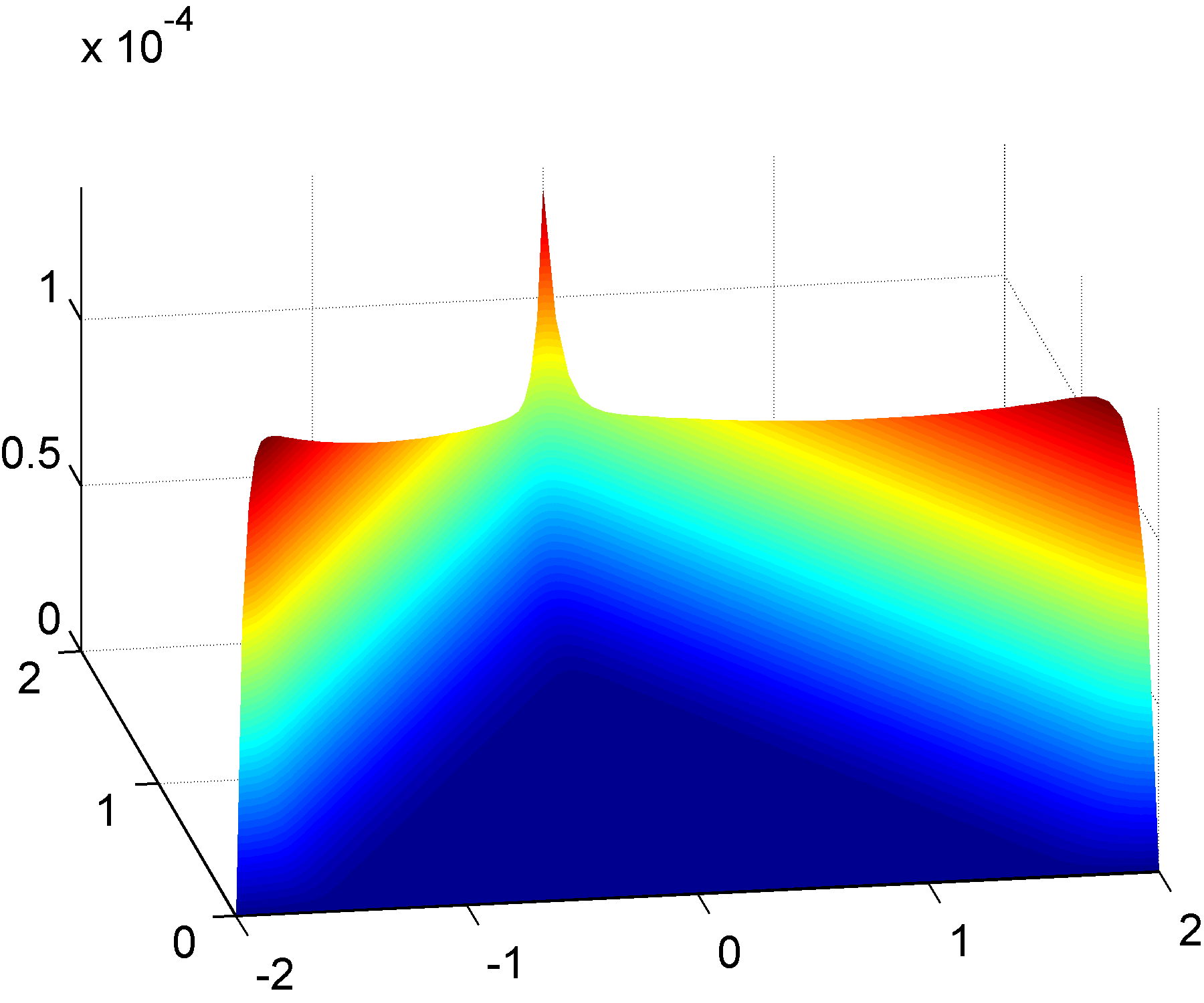
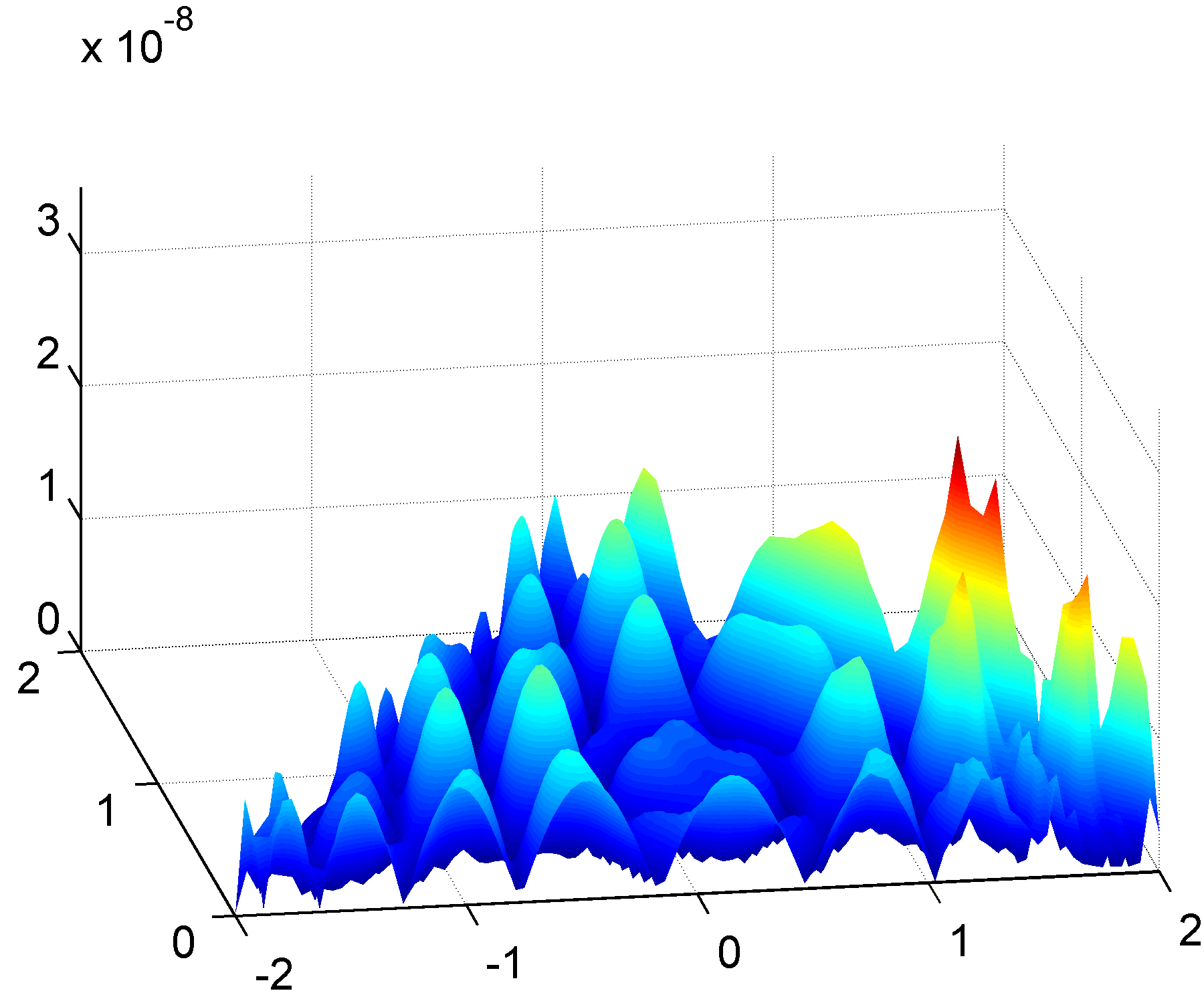
Figure 3: The distribution of the absolute error of the approximate solutions of the Cauchy problem from Example 35 computed according to Proposition 28 with the $f$-polynomials of order $n=20$ and generalized Taylor coefficients (on the left) and with the $f$-polynomials of order $11$ (for $g$) and $18$ (for $h$) with the coefficients obtained by the Remez algorithm (on the right).

Example 36

In this example we consider the same problem (56), (57), again with $b=2$ and $\lambda_{1}=1$ but now with another value of $c$, $c=5i$. Again we have the generalized Taylor coefficients in a closed form (58) and (59) but application of the Remez algorithm encounters an obstacle. As the function $f(x)=e^{cx}$ is complex valued (see Remark 33) the same is true for the functions $\varphi_{k}$ meanwhile as was explained in Section 6 the Remez algorithm is directly applicable only to real valued functions.

Here in order to find the coefficients of the $f$-polynomials from Proposition 28 by a distinct from the generalized Taylor formula method we solve the corresponding linear programming problem as explained at the end of Section 6.

How well the approximation based on the generalized Taylor formula works is shown in Figures 4 and 6 where the distribution of the absolute error of approximation is depicted for $g$, $h$ and the solution $u$ respectively in the case $n=50$.

Figure 4: Graphs of $\left|g-P_{50}\right|$ (on the left) and $\left|h-Q_{49}\right|$ (on the right) from Example 36 with the coefficients $\alpha_{k}$ and $\beta_{k}$ obtained by (48) which in this case reduces to (58) and (59).

The corresponding results obtained by solving the linear programming problem (again, due to the limitation of the machine precision we used $n=14$ for the approximation of $g$ and $n=25$ for the approximation of $h$) are presented in Figures 5 and 6.

Figure 5: Graphs of $\left|g-P_{14}\right|$ (on the left) and $\left|h-Q_{25}\right|$ (on the right) from Example 36 with the coefficients $\alpha_{k}$ and $\beta_{k}$ obtained by solving a linear programming problem.

Figure 6: The distribution of the absolute error of the approximate solutions of the Cauchy problem from Example 36 computed according to Proposition 28 with the $f$-polynomials of order $n=50$ and generalized Taylor coefficients (on the left) and with the $f$-polynomials of order $14$ (for $g$) and $25$ (for $h$) with the coefficients obtained by solving a linear programming problem (on the right).

Example 37

In our final example a variable coefficient equation is considered. Namely, we solve the following Cauchy problem

$$\square u-x^{2}u =0,\quad-b\leq x\leq b,\quad t\geq 0,$$ (60)

$$u(x,0) =g(x)=e^{x^{2}/2}\biggl{(}1+\int_{0}^{x}e^{-s^{2}}ds\biggr{)},$$ (61)

$$u_{t}(x,0) =h(x)=xe^{x^{2}/2}.$$ (62)

Its exact solution is given by the expression

$$u(x,t)=g(x)\cosh t+h(x)\sinh\sqrt{3}t$$

The corresponding ordinary second-order equation has the form

$$f^{\prime\prime}-x^{2}f=0.$$ (63)

The functions $g$ and $h$ are solutions of the equation

$$v^{\prime\prime}-x^{2}v=\lambda v\text{ }$$

with $\lambda=1$ and $\lambda=3$, respectively and hence again we have in our disposal the possibility to write down the coefficients $\alpha_{k}$ and $\beta_{k}$ from (45) explicitly. We compute a particular solution $f$ of (63) numerically using the SPPS method as described in [18], then compute the functions $\varphi_{k}$ and the corresponding coefficients $\alpha_{k}$ and $\beta_{k}$ analogously to Example 35. The result for $n=20$ is presented by Figures 7 and 8 where the error of approximation of $g$, $h$ and $u$ is depicted.

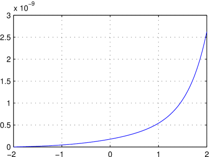
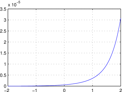
Figure 7: Graphs of $\left|g-P_{20}\right|$ (on the left) and $\left|h-Q_{19}\right|$ (on the right) from Example 37 with the exact generalized Taylor coefficients (48).

Application of the Remez algorithm delivers the following results. The functions $g$ and $h$ were approximated by $f$-polynomials of order $16$ and $19$ respectively and the distribution of the absolute error of the approximate solution of (60)–(62) is depicted on Figure 8. As can be observed with this relatively small number of functions $\varphi_{k}$ involved in the approximation a remarkable accuracy in the final solution is achieved of the order $10^{-14}$.

Figure 8: The distribution of the absolute error of the approximate solutions of the Cauchy problem from Example 37 computed according to Proposition 28 with the $f$-polynomials of order $n=20$ and generalized Taylor coefficients (on the left) and with the $f$-polynomials of order $16$ (for $g$) and $19$ (for $h$) with the coefficients obtained by the Remez algorithm (on the right).

References

- [1] I. Barrodale, L. M. Delves and J. C. Mason Linear Chebyshev Approximation of Complex-Valued Functions. Math. Comput., 32 (1978), 853–863.
- [2] L. Bers Theory of pseudo-analytic functions (New York University, 1952).
- [3] H. Campos, V. V. Kravchenko, S. M. Torba Transmutations, L-bases and complete families of solutions of the stationary Schrödinger equation in the plane. J. Math. Anal. Appl. 389 (2012), no. 2, 1222–1238.
- [4] E. W. Cheney, Introduction to Approximation Theory, 2nd ed., Chelsea, New York, 1986.
- [5] J. Delsarte and J. L. Lions, Transmutations d’opérateurs différentiels dans le domaine complexe. Comment. Math. Helv. 32 (1956), 113–128.
- [6] R. A. DeVore and G. G. Lorentz Constructive Approximation. Berlin: Springer-Verlag, 1993, x + 449 p.
- [7] V. K. Dzyadyk Introduction to the theory of uniform approximation of functions by polynomials. Moscow: Nauka, 1977 (in Russian).
- [8] M. K. Fage and N. I. Nagnibida The problem of equivalence of ordinary linear differential operators. Novosibirsk: Nauka, 1987 (in Russian).
- [9] B. Fischer and J. Modersitzki An algorithm for complex linear approximation based on semi-infinite programming. Numerical Algorithms 5 (1993) 287–297.
- [10] K. Glashoff and K. Roleff A new method for Chebyshev approximation of complex-valued functions, Math. Comput., 36 (1981), 233–239.
- [11] W. G. Kelley, A. C. Peterson The Theory of Differential Equations: Classical and Qualitative. Springer, 2010.
- [12] V. V. Kovtunets Algorithm for computing the best approximation polynomial of the complex-valued function. Issledovaniya po teorii approximacii funkcij (Researchs on Function Approximation Theory), Kiev, Inst. of Mathematics Publ., 1987, 35–42 (in Russian).
- [13] V. V. Kovtunets Algorithm for computing the best approximation polynomial of the complex-valued function on the compact set, Nekotorye voprosy teorii priblizheniya funkcij i ih prilozheniya (Some problems of approximation theory and its applications), Kiev, Inst. of Mathematics Publ., 1988, 71–78 (in Russian).
- [14] V. V. Kravchenko A representation for solutions of the Sturm-Liouville equation. Complex Variables and Elliptic Equations, 2008, v. 53, 775-789.
- [15] V. V. Kravchenko Applied pseudoanalytic function theory. Basel: Birkhäuser, Series: Frontiers in Mathematics, 2009.
- [16] V. V. Kravchenko On the completeness of systems of recursive integrals. Communications in Mathematical Analysis, Conf. 03, 2011, 172–176.
- [17] V. V. Kravchenko, S. Morelos and S. Tremblay Complete systems of recursive integrals and Taylor series for solutions of Sturm-Liouville equations. Mathematical Methods in the Applied Sciences, v. 35, 2012, issue 6, 704–715.
- [18] V. V. Kravchenko and R. M. Porter Spectral parameter power series for Sturm-Liouville problems. Mathematical Methods in the Applied Sciences 2010, v. 33, 459-468.
- [19] V. V. Kravchenko, D. Rochon, S. Tremblay On the Klein-Gordon equation and hyperbolic pseudoanalytic function theory. J. of Phys. A, 2008, v. 41 issue 6, 065205.
- [20] V. V. Kravchenko and S. M. Torba Transmutations for Darboux transformed operators with applications. J Phys A, v. 45, 2012, issue 7, # 075201 (21 pp.)
- [21] V. V. Kravchenko and S. M. Torba Transmutations and spectral parameter power series in eigenvalue problems. To appear in Operator Theory: Advances and Applications.
- [22] M. A. Lavrentiev and B. V. Shabat Problems of hydrodynamics and their mathematical models. Moscow: Nauka, 1973 (in Russian).
- [23] B. M. Levitan Inverse Sturm-Liouville problems. VSP, Zeist, 1987.
- [24] J. L. Lions Solutions élémentaires de certains opérateurs différentiels à coefficients variables. Journ. de Math. 36 (1957), Fasc 1, 57–64.
- [25] V. A. Marchenko Sturm-Liouville operators and applications. Basel: Birkhäuser, 1986.
- [26] V. Matveev and M. Salle Darboux transformations and solitons. N.Y. Springer, 1991.
- [27] G. Meinardus Approximation of Functions: Theory and Numerical Methods, New York: Springer, 1967. Expanded English translation of the German version: Approximation von Funktionen und ihre Numerische Behandlung. Springer Tracts in Natural Philosophy, Volume 4, 1964.
- [28] A. E. Motter and M. A. Rosa Hyperbolic calculus. Advances in Applied Clifford Algebras, 1998, v. 8, No. 1, 109-128.
- [29] Y. Pinchover and J. Rubinstein An introduction to partial differential equations. Cambridge University Press, 2005.
- [30] A. D. Polyanin Handbook of linear partial differential equations for engineers and scientists. Boca Raton: Chapman & Hall/CRC, 2002.
- [31] E. Ja. Remez Fundamentals of numerical methods of Tchebyshev approximation. Kiev: Naukova dumka, 1969 (in Russian).
- [32] J. R. Rice The Approximation of Functions, Vol. 1. Linear theory. Reading, Massachusetts: Addison-Wesley, 1964.
- [33] T. J. Rivlin An introduction to the approximation of functions. Blaisdell: Waltham, Mass., 1969.
- [34] T. J. Rivlin and H. S. Shapiro A unified approach to certain problems of approximation and minimization, J. Soc. Indust. Appl. Math., 9 (1961), 670–699.
- [35] V. I. Smirnov and N. A. Lebedev Functions of Complex Variables: Constructive Theory, Moskow: Nauka, 1964 (in Russian). English translation in V. I. Smirnov and N. A. Lebedev. Functions of Complex Variables: Constructive Theory, MIT Press, Cambridge, MA, 1968.
- [36] P. T. P. Tang A fast algorithm for linear complex Chebyshev approximation. Math. Comput., 52 (1988), 721–739.
- [37] A. F. Timan Theory of Approximation of Functions of a Real Variable, Moskow, 1960 (in Russian). English translation in A. F. Timan, Theory of Approximation of Functions of a Real Variable, New York: Macmillan, 1963.
- [38] K. Trimeche Transmutation operators and mean-periodic functions associated with differential operators. London: Harwood Academic Publishers, 1988.
- [39] V. S. Vladimirov Equations of mathematical physics. Moskva: Nauka, 1981 (in Russian), English translation in V.S. Vladimirov. Equations of mathematical physics (2nd English ed.), Moscow: Mir Publishers, 1983.
- [40] G. A. Watson Numerical methods for Chebyshev approximation of complex-valued functions, in Algorithms for Approximation II, J. C. Mason and M. G. Cox, eds., Chapman and Hall, London, 1989, 246–264.