On the extraction of zero momentum form factors on the lattice
Abstract
We propose a method to expand correlation functions with respect to the spatial components of external momenta. From the coefficients of the expansion it is possible to extract Lorentz–invariant form factors at zero spatial momentum transfer avoiding model dependent extrapolations. These objects can be profitably calculated on the lattice. We have explicitly checked the validity of the proposed procedure by considering two-point correlators with insertions of the axial current, the form factors of the semileptonic decay of pseudoscalar mesons, and the hadronic vacuum polarization tensor entering, for example, the lattice calculation of the anomalous magnetic moment of the muon.
I introduction
Physical observables are calculated on the lattice by extracting hadronic matrix elements from the large euclidean time behavior of correlation functions. The matrix elements are Lorentz–covariant quantities, i.e. tensors of a certain rank and with definite properties under discrete symmetries. These are parametrized in terms of form factors, the Lorentz–invariant coefficients associated with the decomposition on a certain basis. The basis is built by considering products of external momenta, polarization vectors, metric tensor, etc. The form factors multiplying powers of the the external momenta are difficult to extract when these variables vanish.
The class of problems we address in this letter can be exemplified as follows
| (1) |
where is the quantity that can be computed directly on the lattice (a correlator or a combination of correlators), is the quantity one is interested in, while the dots represent additional arguments that may or may not be present and that characterize the given observable.
Typically it is possible to obtain good numerical precision on the form factors for values of in a limited range. Lattice correlators tend to be extremely noisy for large values of the modulus of . On the other side, although the use of flavour twisted boundary conditions Bedaque:2004kc ; deDivitiis:2004kq allows to overcome the quantization of spatial momenta on finite volumes and to compute for very small values of , the numerical signal for goes to zero for nearly vanishing values of and the results in this region are again very rough. In particular there are situations in which one is interested in the value of at that, by using standard lattice techniques, can only be obtained by recurring to (model dependent) extrapolations.
A concrete example of this kind is offered by the calculation at zero recoil of all the independent form factors parameterizing the semileptonic decays Hashimoto:1999yp ; de Divitiis:2007ui ; de Divitiis:2007uk ; deDivitiis:2008df ; Bernard:2008dn .
Another phenomenologically relevant example is given by the hadronic vacuum polarization contribution to the muon that is extracted from the integrated two–point correlator of the electromagnetic currents of the quarks,
| (2) | |||||
In this case the accurate knowledge of is extremely important because divergent contributions are canceled by extracting the physical information from the difference . By using standard approaches, can only be obtained by extrapolating the results at non vanishing and by relying on fitting formulae that unavoidably introduce systematic errors (see ref. Aubin:2012me for a recent discussion of this point).
In this work we discuss a method to be used in order to solve the class of problems discussed above. The method allows to calculate directly on the lattice the th-derivative of a lattice correlator with respect to external spatial momenta. By using the notation of the previous formulae, we shall describe in the following sections a procedure to calculate on the lattice the left hand side of (no sum over )
| (3) |
directly at without the need of any extrapolation and related ansatz for the fitting function. The same problem was also addressed in refs. Aglietti:1994nx ; Lellouch:1994zu with a solution different from the one proposed in this paper.
By applying this method it is possible to compute on the lattice the vacuum polarization scalar form factor at zero momentum according to
| (4) |
II Expansion of the correlators
In order to expand lattice observables in powers of external spatial momenta, let us start by considering a generic correlator depending upon ,
| (5) | |||||
In previous expressions represents the gauge “probability density” and incorporates the fermionic determinants together with the normalization factor of the functional integral. Note that does not depend upon external momenta. Our method consists in expanding , i.e. the correlator at fixed QCD gauge background, with respect to according to
The coefficients can be interpreted as the derivatives of the original correlator with respect to the external momenta. Note that this is true also when the external momenta are quantized as a consequence of the finite volume and of the boundary conditions satisfied by the quark and gauge fields.
After fermionic integration and Wick contractions the lattice correlator can be expressed as the product of quark propagators and operator insertions, i.e.
Here represent a generic operator insertion (see section IV below) while is one of the fermion propagators entering the expression of the given correlator. The fermion propagator ( in short) satisfies the following equation
| (8) |
where is the lattice Dirac operator used to discretize the quarks action. The propagator introduced above ( in short) is simply given by
| (9) |
The previous definition has been made because it is useful to obtain directly, i.e. by solving the lattice Dirac equation with the link variables rescaled by a phase factor
| (10) |
Note that is defined analogously to a lattice propagator associated with a quark field satisfying flavour twisted boundary conditions Bedaque:2004kc ; deDivitiis:2004kq , with the difference that now is not a continuous variable. In this work we shall use periodic boundary conditions for all the quark fields and, consequently, we shall always work within a unitary setup and with the spatial momenta quantized according to
| (11) |
Expressions for the coefficients can now be readily obtained by expanding the lattice propagators and possibly non ultra-local operators entering into the original expression of (see the following sections for examples) in powers of the external momenta. Indeed, since the quark determinants do not depend upon external momenta, the derivatives of the correlator do not involve additional disconnected fermionic Wick contractions with respect to the ones originally present to define .
III Expansion of the propagators
The expansion of the quark propagators can be obtained by starting from the expansion of the lattice Dirac operator,
and by using the identity leading to
| (13) |
In the previous expressions there is no sum over and we have used the following compact notation
| (14) |
For our numerical calculations we have used clover Wilson fermions, corresponding to the specific Dirac operator given below
where , , is the clover definition of the lattice gluon field strength tensor and is the Sheikholeslami–Wohlert coefficient Sheikholeslami:1985ij . The th-derivatives of this operator are proportional either to the “point–split” vector current (for odd ), or to the “tadpole” current (for even ),
| (19) |
where the expressions of the two currents are given by
Graphically, the expansion of the propagator of eqs. (13) can be represented as the sum of iterated insertions at zero momentum of the operators and according to (no sum over )
| (22) |
In the previous expressions we have introduced the following graphical notation
| (23) |
that we shall repeatedly use also in the following sections.
IV Expansion of the vertices
As discussed above, the expression of a correlator at fixed QCD gauge background involves products of traces of propagators and operators , as rewritten here below in a very compact notation,
If the operators are not ultra–local and connect different lattice points, they may also carry a dependence upon . For this reason we have used in previous expression the notation . In these situations the calculation of the coefficients of the momentum expansion of the correlators requires the knowledge of the derivatives with respect to external momenta of all -dependent objects, including the vertices, as shown below for the first derivative
One relevant example of -dependent operator is just given by the point–split vector current discussed above. It undergoes the following expansion
to which, in the case of the integrated insertions of these operators, we associate the following graphical representation
| (26) | |||||
The previous expressions will be used below in order to expand the integrated correlator proportional to the vacuum polarization tensor.
V Applications
In this section we check the validity of the method by calculating on the lattice the derivatives with respect to external spatial momenta of a set of correlation functions.
We start by considering two-point correlators of a pseudoscalar density and of an axial current. This example has no relevance from the phenomenological point of view but it is very useful to explain how the method works in practice and to check its effectiveness in a simple and controllable situation. As a second application we consider three-point correlation functions and use our method to extract at zero recoil both form factors parametrizing pseudoscalar–to–pseudoscalar semileptonic transitions. Finally we compute the second derivative of the vacuum polarization tensor and extract the scalar form factor needed for the muon calculation directly at zero momentum.
The numerical results have been obtained (on a single volume, at fixed lattice spacing and fixed sea quark mass in the theory) in order to check the validity of the proposed procedure. For this reason, also in the case of the phenomenologically relevant applications discussed below, we do not quote numbers in physical units neither attempt to estimate possible systematic errors.
For our numerical investigations we have used the gauge configurations corresponding to the and ensembles of the CLS initiative. These in turn correspond to the simulation parameters , , and to the lattice volumes and . The larger volume will only be used, in the case of the vacuum polarization tensor, for a test of the method performance with increasing volumes. All the other information concerning these gauge ensembles can be found in refs. DelDebbio:2006cn ; DelDebbio:2007pz .
V.1 Two–point correlation functions
A simple and illustrative check of our procedure have been obtained by considering the following two–point correlators
For large euclidean time separations we can neglect sub–leading exponentials contributing to the correlators and write
| (28) |
where is the momentum of the pseudoscalar meson, its mass, its energy while and are Lorentz-invariant form factors depending upon the meson mass square .
In this simple situation our method is not needed because the decay constant of the meson can easily be extracted from the correlators and both evaluated at vanishing spatial momentum. On the other hand, we can check our proposal by computing the first coefficient of the momentum expansion of , namely (no sum over )
| (29) |
where, according to the formulae derived in the previous sections, we have
We remark that the quantities above have been determined in the periodic theory with or, equivalently, . The product of propagators appearing in the previous expressions can be conveniently obtained by using the sequential source method, i.e. by using as the source vector for a new inversion.
The large time behavior of is now expected to be
| (31) |
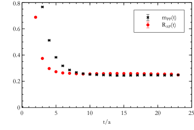
In order to check this behavior, in FIG. 1 we compare the ratio
| (32) |
with the effective mass extracted from the pseudoscalar–pseudoscalar correlator at zero spatial momentum. As it can be seen, for large time separations there is agreement within the statistical errors between the two definitions of effective mass, thus confirming the theoretical expectations and the validity of our method.
An important remark is in order here. Once a given correlator it has been made finite by multiplying it with the appropriate renormalization factors, the derivatives of the renormalized correlation functions with respect to external momenta are also finite, i.e. there is no need of specific renormalization prescriptions for the coefficients of the momentum expansion. In particular, the ratio is finite (renormalization factors identically cancel between the numerator and the denominator) and has indeed been plotted in FIG. 1 without multiplying it with any factor.
V.2 Three–point correlation functions
In this section we apply our method to three–point correlation functions. In particular we consider the form factors entering the rate of the semileptonic decay of a pseudoscalar meson into another pseudoscalar meson, . The process is mediated by the vector part of the weak current and the corresponding matrix element can be parametrized in terms of two independent Lorentz-invariant form factors,
where and are respectively the initial and final momenta of the hadrons and
| (34) |
Here and in the following the dependence of form factors upon Lorentz invariants is understood, with and .
The form factors are usually extracted by considering ratios of three-point correlators evaluated at different initial and final masses and momenta. By introducing a compact notation for the initial, final and spectator quark propagators ( are the quark masses),
| (35) |
these correlators can be written as follows
| (36) |
In the previous expression the distance between the interpolating operators of the initial and final pseudoscalar mesons has been set to half of the time extent of the lattice, i.e. , we have called , the improvement of the vector current has been neglected and the multiplicative renormalization factors of the interpolating pseudoscalar densities and of the local vector current have been omitted because these cancel in the ratios from which the form factors are extracted (see below).
Our gauge ensemble has been generated with two dynamical quarks having the same mass while in eq. (36) we are referring to three different quark flavours. The third quark, in the case of different initial and final meson masses, has been treated in the quenched approximation.
When the masses of the initial and final mesons are equal, the conservation of the vector current implies the presence of a single form factor
| (37) |
exactly normalized to 1 at . The simple situation of equal initial and final meson masses at zero recoil has no phenomenological relevance but gives us the opportunity of repeating the check already performed in the case of two–point correlators also in the case of three–point correlation functions. To this end, we set the initial spatial momentum to zero, , and consider the behavior of the correlators for large relative time separations by neglecting sub–leading exponentials,
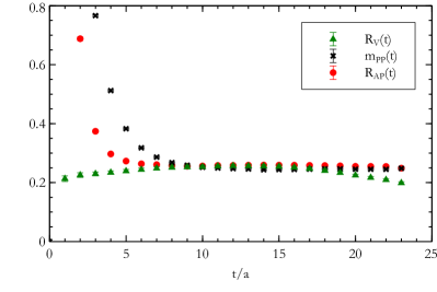
where , is the spatial momentum of the final meson, its energy and the matrix element of the interpolating operator. We have computed the first coefficient of the momentum expansion of , i.e. (no sum over )
| (39) |
and we have considered the ratio
| (40) |
For large time separations is expected to be equal to the meson mass and, by setting the quark masses equal to the ones used in the previous section, it is possible to compare with and . The comparison is shown in FIG. 2. As it can be seen the three definitions of effective meson mass agree within the statistical errors in the middle of the lattice where the large time separation condition is satisfied also for .
We now come to the phenomenological relevant situation in which the masses of the two mesons are different. In this case the determination of the two independent form factors can be achieved by solving the following linear system of equations,
The previous system becomes critical at the maximal value of , i.e. in the zero recoil situation . In this case the first equation can be used to obtain a single combination of and that is proportional to defined here below (see ref. Hashimoto:1999yp )
The previous parametrization is widely used when the initial and final hadrons are both heavy–light pseudoscalar mesons (for example in the case) and the form factors are considered as functions of
| (43) |
The zero recoil point at corresponds to .
By applying our method it is possible to obtain both the form factors directly at . To this end it is useful to consider (by neglecting sub–leading exponentials)
In previous expressions one of the quark lines has been drawn with a different color (green) in order to represent a quark of different mass with respect to the others (in particular in the numerical analysis we have set to be compared with ). By relying on the hermiticity of the vector current we also get
By using these relations, together with the corresponding ones in the case of coinciding initial and final external states we get
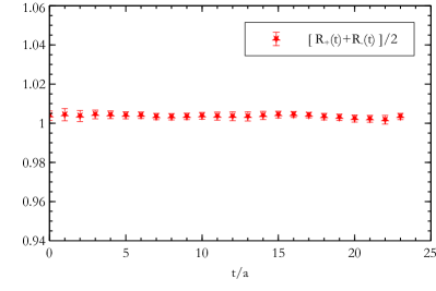
The effective form factors are then obtained from
| (47) |
The combinations of correlators given in previous relations is particularly effective in minimizing statistical fluctuations that cancel between the different factors. In particular, when the initial and final meson masses are equal, the normalization conditions and are identically verified for each gauge configuration of the given ensemble. To give an idea of the plateaux that can be obtained by using this method we show in FIG. 3 the effective form factors extracted from our data.
V.3 The vacuum polarization tensor
In this section we show how the momentum expansion can profitably be used in order to calculate the hadronic vacuum polarization tensor, a quantity which is needed in order to predict the leading hadronic contribution to the anomalous magnetic moment of the muon.
The hadronic vacuum polarization tensor is calculated on the lattice by considering the integrated two–point correlator of the electromagnetic currents of the quarks
| (48) | |||||
where . Given our choice of lattice Dirac operator, we have used the point–split vector currents in order to define the electromagnetic currents of the quarks,
| (49) |
We have chosen the momentum routing in which the external momentum flows through one of the two quark propagators. With this choice the point–split vector currents at the vertices connect two fermion lines with different momentum and, consequently, bring the dependence upon .
The leading hadronic contribution to the of the muon is obtained by extracting the scalar form factor from eq. (48) and by considering the difference . The subtracted form factor is introduced in order to cancel divergent contributions (see for example refs. Gockeler:2003cw ; Aubin:2006xv ; DellaMorte:2011aa ; Feng:2011zk ; Boyle:2011hu for dedicated works) and, for this reason, it is very important to have an accurate determination of . By using standard techniques, can only be obtained by extrapolating the data obtained at . These extrapolations unavoidably introduce systematic errors (for a recent discussion of this point see Aubin:2012me ). In the following we shall show how can be computed on the lattice directly and without the need of any extrapolation.
As for the other quantities computed in this paper, the results for have been obtained with limited statistics, on a single volume, at fixed quark masses, etc. in order to demonstrate the effectiveness of the proposed procedure. For this reason we shall not use our results to make a prediction for the muon . This will be the subject of future work.
After fermion integration and Wick contractions, the correlator has both fermion–connected and fermion–disconnected contributions. If, for example, we limit ourself to the case in the isospin symmetric theory we have
| (50) |
where and . In the following we shall concentrate on the connected part. Actually, many of the lattice collaborations involved in the computation of the hadronic vacuum polarization tensor Gockeler:2003cw ; Aubin:2006xv ; DellaMorte:2011aa ; Feng:2011zk ; Boyle:2011hu have neglected (or just attempted an estimate of) disconnected contributions. The choice is due to the big computational effort required for the calculation and not because these are expected (at least in general) to be negligible. Our method has to be generalized for disconnected diagrams.
In the following we call the connected contribution corresponding to a single quark without multiplying it for the corresponding electric charge. In particular, we consider the correlators with different spatial indices () because these are proportional to the spatial momenta and because they do not require additional contributions in order to satisfy gauge Ward identities. Indeed, the lattice photon self energy with equal indices includes also the tadpole graph, where two photons couple to the fermion line in a single vertex (the current coupled to two photons is the one that we have previously indicated as “tadpole current”). We checked anyway, on limited statistics, that the gauge Ward identities are satisfied.
First, fixed and , we have computed the integrated correlation at and and divided it by the momenta,
| (51) |
Then we have applied the rules discussed in the previous sections to define the second mixed derivative, acting on propagators and vertices and evaluated at zero momentum, according to
| (52) |
where, for sake of brevity, we have dropped position arguments and we have used the relations
| (53) |
to obtain the derivative of the vertices (see section IV above). Note that in the previous expressions the factor appears because the currents here depend upon and not upon .
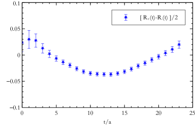
To the lattice definition of , eq. (52), it can be given the following graphical representation (see also eq. (22))
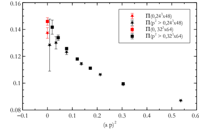
In FIG. 4 we show our results. The black points correspond to obtained from eq. (51) and, as expected, tend to be noisy for small values of . The red points correspond to calculated directly on the lattice according to eq. (52). The data, obtained with limited statistics ( gauge configurations for the ensemble and gauge configurations for the ensemble), correspond to two different lattice volumes ( and ) and differ at small momenta for finite volume effects.
For each data set, the error on is comparable to the error that can be obtained at but, coming from a direct calculation, it does not need to be corrected for systematic errors due to extrapolations and, important to note, it scales with the statistics. Furthermore, the error on scales favorably with the lattice volume.
VI Conclusions
The method discussed in this letter allows the direct calculation on the lattice of the derivatives of correlators with respect to external momenta. We have described the method and checked its validity for several correlation functions.
In particular, we have derived expressions to be used in order to compute both form factors parametrizing semileptonic decays of pseudoscalar mesons into other pseudoscalar mesons, directly at zero recoil. These relations, checked numerically in this paper, may have many important phenomenological applications, for example in the calculation of differential decay rate without excluding the case, etc. Similar relations can be easily derived along the lines discussed in this paper for the pseudoscalar-to-vector channels.
Another important application of the method concerns the direct calculation of the scalar form factor needed to predict the hadronic vacuum polarization contribution to the muon anomalous magnetic moment. In particular our method, as explicitly shown in the paper, allows to obtain without the need of any extrapolation and related systematic uncertainties.
The method is general, easy to implement, and we are pretty confident it will find several applications in the field of lattice phenomenology.
Acknowledgements.
We thank F. Sanfilippo for useful discussions, our colleagues of the CLS initiative for sharing the efforts of the generation of the gauge configurations used in this work and MIUR for partial support under the contract PRIN09.References
- (1) U. Aglietti, G. Martinelli and C. T. Sachrajda, Phys. Lett. B 324 (1994) 85 [hep-lat/9401004].
- (2) L. Lellouch et al. [UKQCD Collaboration], Nucl. Phys. B 444 (1995) 401 [hep-lat/9410013].
- (3) P. F. Bedaque, Phys. Lett. B593 (2004) 82-88. [nucl-th/0402051].
- (4) G. M. de Divitiis, R. Petronzio, N. Tantalo, Phys. Lett. B595 (2004) 408-413. [hep-lat/0405002].
- (5) S. Hashimoto, A. X. El-Khadra, A. S. Kronfeld, P. B. Mackenzie, S. M. Ryan and J. N. Simone, Phys. Rev. D 61 (1999) 014502 [hep-ph/9906376].
- (6) G. M. de Divitiis, E. Molinaro, R. Petronzio and N. Tantalo, Phys. Lett. B 655 (2007) 45 [arXiv:0707.0582 [hep-lat]].
- (7) G. M. de Divitiis, R. Petronzio and N. Tantalo, JHEP 0710 (2007) 062 [arXiv:0707.0587 [hep-lat]].
- (8) G. M. de Divitiis, R. Petronzio and N. Tantalo, Nucl. Phys. B 807 (2009) 373 [arXiv:0807.2944 [hep-lat]].
- (9) C. Bernard, C. E. DeTar, M. Di Pierro, A. X. El-Khadra, R. T. Evans, E. D. Freeland, E. Gamiz and S. Gottlieb et al., Phys. Rev. D 79 (2009) 014506 [arXiv:0808.2519 [hep-lat]].
- (10) C. Aubin, T. Blum, M. Golterman and S. Peris, arXiv:1205.3695 [hep-lat].
- (11) B. Sheikholeslami and R. Wohlert, Nucl. Phys. B 259 (1985) 572.
- (12) L. Del Debbio, L. Giusti, M. Luscher, R. Petronzio and N. Tantalo, JHEP 0702 (2007) 056 [hep-lat/0610059].
- (13) L. Del Debbio, L. Giusti, M. Luscher, R. Petronzio and N. Tantalo, JHEP 0702 (2007) 082 [hep-lat/0701009].
- (14) M. Gockeler et al. [QCDSF Collaboration], Nucl. Phys. B 688 (2004) 135 [hep-lat/0312032].
- (15) C. Aubin and T. Blum, Phys. Rev. D 75 (2007) 114502 [hep-lat/0608011].
- (16) M. Della Morte, B. Jager, A. Juttner and H. Wittig, JHEP 1203 (2012) 055 [arXiv:1112.2894 [hep-lat]].
- (17) X. Feng, K. Jansen, M. Petschlies and D. B. Renner, Phys. Rev. Lett. 107 (2011) 081802 [arXiv:1103.4818 [hep-lat]].
- (18) P. Boyle, L. Del Debbio, E. Kerrane and J. Zanotti, Phys. Rev. D 85 (2012) 074504 [arXiv:1107.1497 [hep-lat]].